Détection et classification dans un contexte acoustique passive : application à la détection des signaux basse-fréquences des baleines bleues

(1)

HAL Id: tel-02475688

https://tel.archives-ouvertes.fr/tel-02475688

Submitted on 12 Feb 2020

HAL is a multi-disciplinary open access archive for the deposit and dissemination of sci-entific research documents, whether they are pub-lished or not. The documents may come from teaching and research institutions in France or abroad, or from public or private research centers.

L’archive ouverte pluridisciplinaire HAL, est destinée au dépôt et à la diffusion de documents scientifiques de niveau recherche, publiés ou non, émanant des établissements d’enseignement et de recherche français ou étrangers, des laboratoires publics ou privés.

passive : application à la détection des signaux

basse-fréquences des baleines bleues

Lea Bouffaut

To cite this version:

Lea Bouffaut. Détection et classification dans un contexte acoustique passive : application à la dé-tection des signaux basse-fréquences des baleines bleues. Acoustics [physics.class-ph]. Université de Bretagne occidentale - Brest, 2019. English. �NNT : 2019BRES0057�. �tel-02475688�

(2)

THESE DE DOCTORAT DE

L'UNIVERSITE

DE

BRETAGNE

OCCIDENTALE

COMUE UNIVERSITE BRETAGNE LOIRE

ECOLE DOCTORALE N°598 Sciences de la Mer et du littoral

Spécialité : Acoustique sous-marine et Traitement du signal

Detection and classification in passive acoustic contexts:

Application to blue whale low-frequency signals

Thèse présentée et soutenue à Lanvéoc, le 22 Octobre 2019

Unité de recherche : Institut de Recherche de l'Ecole Navale IRENav – EA 3634

Par

Léa BOUFFAUT

Rapporteurs avant soutenance : Olivier ADAM,

Professeur des Universités,

Institut ∂_{’Alembert, Sorbonne Université}

Jérôme MARS,

Professeur des Universités, Gipsa-Lab, Université de Grenoble

Composition du Jury :

Rapporteurs :

Olivier ADAM, Professeur des Universités, Institut ∂_{’Alembert, Sorbonne Université}

Jérôme MARS, Professeur des Universités, Gipsa-Lab, Université de Grenoble

Examinateurs :

Jean-Yves ROYER, Directeur de Recherche CNRS, Président du jury, LGO, Institut Universitaire Européen de la Mer, UBO

Abdeldjalil AISSA-EL-BEY, Professeur, Lab-STICC, Institut Mines Télécom Atlantique Holger KLINCK, Directeur de Recherche (Ph. D), Cornell Lab of Ornithology, Cornell University Odile GERARD, Ingénieure (Dr.)

DGA Techniques Navales, Toulon

Co-encadrante de thèse :

Valérie LABAT, Maître de Conférences, IRENAv - Ecole Navale

(3)

(4)

Thèse de doctorat

pour obtenir le grade de docteur délivré par

l’Université de Bretagne Occidentale

Spécialité doctorale “Acoustique sous-marine et traitement du signal”

présentée et soutenue publiquement par

Léa B

OUFFAUT

le Mardi 22 Octobre 2019

Detection and classification in passive acoustic contexts

Application to blue whale low-frequency signals

Jury

Olivier Adam, Professeur des universités Rapporteur

Jérôme Mars, Professeur des universités Rapporteur

Jean-Yves Royer, Directeur de recherche CNRS Examinateur

Abdeldjalil Aissa-El-Bey, Professeur Examinateur

Holger Klinck, Directeur de recherche Examinateur

Odile Gérard, Ingénieure-docteure Examinatrice

Abdel-Ouahab Boudraa, Professeur des universités Directeur

Valérie Labat, Maitre de conférence Encadrante

Institut de Recherche de l’École Navale EA3634 École Navale / Arts et Métiers ParisTech BCRM Brest CC600, 29240 Brest Cedex 9, France

(5)

(6)

Après quatre années qui ont filées comme le vent un soir de tempête sur le pont de Recouvrance, me voila à essayer de résumer en quelques lignes à quel point je suis reconnaissante pour tout le soutien que j’ai reçu. Je dois l’admettre, j’ai vraiment attendu jusqu’à la dernière minute; je n’étais pas sûre de trouver les mots. C’est parti. . .

Pour commencer, un grand merci à mes encadrants Abdel-Ouahab Boudraa et Valérie Labat, pour avoir eu confiance en moi dès le départ, m’avoir suivie et supportée, dans tous les sens du terme, tout au long de cette incroyable odyssée. J’apprécie la liberté que vous m’avez attribuée et le soutien que vous m’avez apporté dans la poursuite de l’ensemble de mes projets, bien sûr scientifiques avec toutes les relectures de dernière minute, mais aussi d’avoir compris et approuvé ma volonté de “voir du pays”. Merci de m’avoir accompagnée dans l’élaboration des différents dossier de financement.

Je tiens aussi à sincèrement remercier Jérôme Mars et Olivier Adam pour avoir accepté de lire et d’évaluer mon manuscrit, ainsi que l’ensemble des membres du jury: Jean-Yves Royer, Abdeldjalil Aissa-el-Bey, Holger Klinck et Odile Gérard pour leurs commentaires constructifs et les riches discussions qui ont suivi la soutenance. Merci d’avoir fait le déplacement jusque notre bout du monde !

Ensuite, un immense merci à Richard Dréo, je ne serai pas allée bien loin sans toi ! Déjà, merci d’avoir eu le génie de faire le lien entre les données sismiques du projet RHUM-RUM et les vocalises des baleines. Merci de t’être embarqué avec moi dans ce projet baleinesque, d’avoir remonté les manches et trouvé la trace de Simone ! Je suis aussi vraiment reconnaissante pour ton rôle de pas si vieux sage et pour l’aide précieuse que tu m’as apportée. Aussi, c’était une super bonne idée d’aller toquer à toutes les portes de la rade. . .

Ce qui m’amène à parler de ceux de l’autre rive: Merci à Flore Samaran et Julien Bonnel, de nous avoir ouvert les portes de l’ENSTA et d’avoir prêté oreille à notre chorus. Flore et Manue, nos discussions et vos super explications m’ont permis de mieux comprendre les problématiques et enjeux passés, présents et futurs des baleines de l’Océan Indien (et d’apprendre une flopée de nouveaux mots!). À votre contact j’ai gagné en humilité, vos expériences ont bousculé mes certitudes et m’ont ouvert les yeux sur la complexité de la PAM. Maëlle, merci d’avoir accepté de passer le détecteur de FX sur nos données pour que je puisse faire la comparaison ! Et merci à

(7)

tous les membres du très officiel Flore Samaran’s lab (Julie, Fabio, Remi . . . ) pour le soutien moral lors de ma fusillade présentation au LAB-STICC et les hilarants déjeuners du Flunch. Laurent, Bazile et Florent, merci d’avoir éclairé ma lanterne sur la propa ASM, les mesures de niveaux etc. Bien qu’éloigné de ne notre terre d’irréductibles Brestois, Guilhem je souhaite te remercier pour nous avoir donné accès à cet incroyable jeu de données et pour tes conseils avisés. Je suis admirative de ta rigueur scientifique, ta réactivité et de ton engagement pour le partage et échanges inter-disciplinaires.

À vous tous, j’espère que nous continueront à collaborer !

Avant de passer en anglais pour dire quelque mots à mes collègues d’outre-Atlantique, il me semble judicieux de remercier ici les financements de mobilité du GdR ISIS et de l’École Navale qui ont rendu ce séjour possible, ainsi que la Fondation de la mer et IEEE OES pour la reconnaissance de ces dits travaux. First, Holger, I could never thank you enough for accepting and welcoming me into your lab. To me, this has been a life-changing experience. It has open my eyes to the meaning and direction I want to give to my work. Shyam, thanks for taking me under your wing, helping me become more accurate in programing and writing. Thanks to both of you for spending a tremendous amount of time editing and improving my English writing skills. I am also grateful that you encouraged me to take a step back from the work to get a better overview and see the whole picture. I would also like to thank each member of the extended CCB community, with a special note to Ana, Michelle, Karolin, David, Nisha, Luciana, Peter, Margherita, Rob, Lauren, Laurel, and Kristin: thanks for the walks in the snow, the enlighten talks about your beautiful country, the good food, drinks and laughs (and pasta making lessons!), game nights and all. I had the most wonderful time with you all. To Shyam, Michelle and Luciana, now that I have some more time, I hope we can get somewhere with our fancy project!

De retour en Brittanie, un petit mot quand même sur l’École Navale qui m’a offert un cadre de travail exceptionnel. Les traversées quotidiennes en transrade commencent déjà à me manquer tant pour les magnifiques levers de soleil, les retours pourchassés par les dauphins ou les parties de tarot trop bruyantes de l’étage. Merci pour les moyens qui ont étés mis à ma disposition pendant ces quatre ans. Merci aussi de m’avoir fait confiance pour contribuer à la formation des élèves, où j’ai pu gagner, je crois, en pédagogie et en assurance.

Une antépénultième escale au labo: merci à tous pour ces quatre années. Merci Christophe pour tes conseils sur les bourses et les poursuites de carrière. Gaël et Amélie merci pour l’organisation bien huilée de la soutenance. À mes copains de galère de la première heure, Loïc et Benjamin, merci de m’avoir fait tellement lever les yeux au ciel que j’ai failli m’en décrocher la mâchoire et d’avoir toujours été là ! Bruno, les g.d. (Flo, Benoit ET Arthur pour une sombre histoire de licorne), Kostas (++ pour avoir été un super co-bureau!), Eulalie, Jishen, Goulven, Guillaume, Tom: merci pour les parties de tarot, les conversation sans queue ni tête de midi, la

(8)

décompression du Tyr, les BBQ et diners en tout genre. Avec un peu de persévérance, j’ai appris à moins vous détester ;)

À ma famille, j’aime où nous en sommes aujourd’hui. Vous ne savez pas ce que cela signifie pour moi de vous avoir vus tous réunis pour ma soutenance. Maman merci pour tout ce que je ne sais pas exprimer et pour ce buffet somptueux. Thib, tu sais où commander quand ton heure sera venue ! Papa et Claudine, le miel m’a suivi jusqu’à mon nouveau chez moi et rend les soirées thé au coin du feu encore plus douces. Nathalie et Quentin merci énormément d’avoir fait le déplacement !

Pour finir, le plus grand des merci à mon amoureux. Merci de toujours croire en moi et d’être le meilleur des supporters. Merci de toujours prêter une oreille attentive à ce que j’ai à dire, de toujours (ok, presque) trouver les mots justes. Merci d’avoir été actionnaire majeur de la SNCF, puis de m’avoir rejoint sur des rives plus septentrionales de l’atlantique et d’être toujours partant pour de nouvelles aventures !

(9)

(10)

Acknowledgments v Contents ix List of Figures xi List of Tables xv Glossary xvii Introduction 1

Publications and communications 7

1 Passive acoustic monitoring of blue whales: survey, study and protect the oceans 9

1.1 Blue whales survey methods . . . 11

1.2 Passive acoustic monitoring equipment. . . 15

1.3 Applications of passive acoustic monitoring . . . 21

1.4 Underwater acoustics . . . 22

1.5 Signal processing . . . 28

1.6 Conclusion. . . 33

2 Low frequency sounds from the bottom of the Indian Ocean 35 2.1 RHUM-RUM data . . . 37

2.2 Low-frequency soundscapes from the bottom of the Indian Ocean. . . 39

2.3 Baleen whale acoustic signatures. . . 45

2.4 Multi-sensor observations . . . 54

3 Detection of stereotyped sounds: the Stochastic Matched Filter 59 3.1 Are received signals random? . . . 61

3.2 Noise reduction problem formulation in the time domain . . . 64

3.3 Matched Filter . . . 65

3.4 Stochastic Matched Filter . . . 67

3.5 Extension of the Stochastic Matched Filter to the passive context . . . 73

(11)

4 Performance analysis of stereotyped sounds detectors 87 4.1 The performance analysis dilemma . . . 88

4.2 Groundtruth dataset context . . . 88

4.3 Method . . . 90

4.4 Performances versus threshold . . . 92

4.5 Performances against the SNR . . . 94

4.6 Discussion . . . 97

5 Automatic transcription 103 5.1 Introduction . . . 105

5.2 Segmentation of blue whale calls. . . 106

5.3 Classification and reconstruction . . . 118

5.4 Results . . . 121

5.5 Discussion . . . 125

(12)

1 Catch and whale number in the southern Ocean. . . 2

2 Schematics of PAM. . . 3

3 Illustration of the problem of detection in a passive context. . . 4

1.1 Blue whale global migratory map and patterns. . . 11

1.2 Unmanned aerial system survey of a humpback whale. . . 12

1.3 Science cover 1971: Songs of Humpback whales. . . 13

1.4 Blue whale song diversity, distribution and representation in the Southern hemi-sphere. . . 14

1.5 Schematics of the different types of PAM recorders. . . 15

1.6 Ari Friedlaender deploys a tag on a humpback whale in Antarctica’s Wilhelmina Bay. 19 1.7 Range of validity of modal and geometrical propagation.. . . 23

1.8 Sound speed profile and influential parameters. . . 23

1.9 Illustration of acoustic ray deviation depending on the sound speed profile. . . 24

1.10 Illustration of different acoustic paths. . . 25

1.11 Propagation simulation. . . 25

2.1 RHUM-RUM seismic network and the Southwest Indian Ridge (SWIR) array in Western Indian Ocean. . . 37

2.2 Picture of a LOBSTER. . . 39

2.3 Illustration of underwater soundscape categories.. . . 40

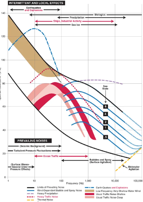
2.4 Wenz curves. . . 41

2.5 Ship traffic in the Indian Ocean. . . 42

2.6 Large ship radiated noise spectrum diagram.. . . 43

2.7 Example of the spectrogram of the noise radiated from ship, recorded by an OBS. . 43

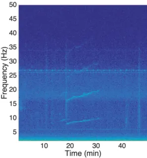
2.8 Earthquake and whale calls. . . 44

2.9 Ice tremor and whale calls. . . 44

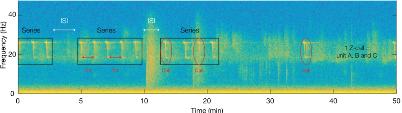
2.10 Illustration of units, call, ICI, series and ISI definitions on an ABW song. . . 46

2.11 Annotated spectrogram of an ABW call. . . 46

2.12 Propagation effect on ABW call series. . . 47

2.13 Annotated spectrogram of a MPBW call. . . 48

2.14 Propagation effect on MPBW call series.. . . 49

2.15 Propagation effect on series of 5 P-calls . . . 50

(13)

2.17 Propagation effect on FW call series. . . 51

2.18 Spectrogram and normalized received levels (dB/Hz) of FW pulses and ABW calls. 52 2.19 Recap of the observed baleen whale calls frequency spans and relative intensities. 54 2.20 Spatio-temporal distribution of baleen whale vocal activity on the RHUM-RUM network. . . 55

2.21 Localization method. . . 56

2.22 Long-term spectrograms of May 2013.. . . 58

3.1 Spectrograms of real and simulated received ABW calls. . . 62

3.2 Scheme of classical SMF offline and online processing. . . . 72

3.3 Spectrum of three filters (H1, H10, HQmax) of the permanent filter bank compared to the spectral representation of the reference signal (HOpt). . . 74

3.4 Comparison between the SMF + MF and MF on a high SNR recording of ABW calls. 79 3.5 Comparison between the SMF + MF and MF on a low SNR recording of ABW calls. 80 3.6 Scuba-diver breathing spectrogram recorded in a tank, fs= 44.1 kHz. . . 82

3.7 Scuba-divers: spectrum of three filters (H1, H10, HQmax) of the permanent filter bank compared to the spectral representation of the reference signal (HOpt). . . . 82

3.8 Application of the SMF to the recording of two scuba-divers in a swimming pool (fs= 96 kHz).. . . 83

3.9 Scheme of the SMF improved for a passive application. . . 85

4.1 ABW passive acoustic monitoring tracking through the SWIR array. . . 89

4.2 ABW of May 31st_{, 2013 dataset temporal evolutions.} _{. . . 90}

4.3 Illustration of detection threshold limits. . . 92

4.4 TPR, MDR and FDR of the MF and the SMF + MF as a function of the detection threshold. . . 93

4.5 ROC comparison between the MF, the SMF + MF and the Z-detector. . . 94

4.6 Precision-Recall comparison between the MF, the SMF + MF and the Z-detector. . 94

4.7 Comparative performance analysis between the MF Ts = 0.01, the SMF +MF Ts = {0.005;0.01;0.016} and, the Z-detector on real data. . . 95

4.8 Time-dependent compared performance analysis of MF, SMF + MF and the Z-detector on a ground truth dataset of 845 annotated calls, on May 31st_{, 2013.}_{. . . . 96}

4.9 Comparison of different SNR estimation methods. . . 98

4.10 Recap of the experimental performances of MF, SMF +MF and, Z-detector.. . . 100

5.1 Illustration of concurrently calling species identified as TF overlapping calls.. . . . 105

5.2 Automatic transcription algorithm flow chart. . . 106

5.3 Illustration of the time and frequency parameters for chirpyness and frequency variation analysis. . . 107

5.4 Illustration of the tonal detectors on ABW and MPBW calls. . . 110

5.5 Illustration of Silbido scoring metrics. . . . 114

(14)

5.7 Tonal units number of instances and distribution in the training dataset, out of

4000 annotated signals. . . 118

5.8 Illustration of features of average frequency and simultaneous frequency ratio on

the training dataset. . . 119

5.9 Training data projected on the first and second PCs. . . 121

5.10 Unsupervised application of the transcription strategy.. . . 124

5.11 Flowchart of the pattern recognition strategy for automatic transcription of BW

(15)

(16)

1.1 Example of the RHUM-RUM OBS characteristics. . . 17

1.2 Example of the OHASISBIO network sound-channel hydrophones characteristics. 17 1.3 Example of the 53-F DIFAR sonobuoys characteristics. . . 18

1.4 Example of the Seaglider™ characteristics.. . . 19

1.5 Example of the DTAG3 characteristics. . . 20

1.6 Baleen whale survey methods recap.. . . 20

1.7 Evolution of the acoustic pressure for plane, spherical and cylindrical wave and their associated geometrical spreading losses. . . 27

1.8 One-class and multi-classes pattern recognition layout. . . 29

2.1 SWIR array OBSs characteristics. . . 39

3.1 ABW call SNRs (dB). . . 78

4.1 Detection theory. . . 91

4.2 Detection range of the MF, SMF + MF and the Z-detector. . . 99

5.1 Analysis of baleen whale call units and partials for chirpyness (Hz/s) and frequency variations. . . 107

(17)

(18)

ABW Antarctic blue whale.ix,x,xiii,2,26,45–47,51–54,56,62,72–74,76,78–80,85,88–91,93,

97,98,100,105–107,110–112,116,119–122,124,127–130

ACF auto-correlation function.108,109

BW blue whale.xi,1–5,11,12,14–16,18,19,21–23,26–31,33,45–47,49,53,61,64,67,101,105,

108,118,124,125,127,129–132

chirpyness rate of frequency change of a signal in Hz/s.x,xiii,106,107

complex tone sound wave consisting of sinusoidal components of different frequencies.48

DCLDE detection, classification, localization and density estimation of marine mammals.31,

128,131

DS down-sweep.47,48,107,119,121,122,124,125,129,130

FDR false discovery rate.x,92–97,100,128

FW Fin whale.ix,x,45,49–54,57,89,106,107,122,123,127

GEP generalized eigenvalue problem.68,69,72,75,130

GMM Gaussian mixture model.120,121,124,125,129,131

HPS harmonic product spectrum.108–112,114,115,117,129

ICI inter-call interval.ix,45–50,53,131

inharmonic frequencies frequencies which are not rational multiples of each other.48

ISI inter-series interval.ix,45–50,53

IWC International whaling commission.ix,2,3

KLE Karhunène-Loève expansion.67–70,120

(19)

MDR missed detection rate.x,91,93,95–97,128

MF matched filter.x,xiii,4,5,29–32,64–68,74,78–81,84,85,88,90–97,99–101,127,128

MPBW Madagascar pygmy blue whale.ix,x,26,45,48,49,54,56,105–107,110–112,116,119,

121–125,127,129,130

nfft Spectrogram number of sampling points.47,49–51,56,58,90

OBS ocean bottom seismometer.ix,xiii,16,33,37–40,43,45–51,53–56,58,62,63,78,79,88–90,

92,97,99,111,112,118,127–130

PAM passive acoustic monitoring.ix,3,5,13–22,26,28–30,32,33,38,49,63,64,66,76,98,124,

125,127,132

partial one of a group of frequencies, not necessarily harmonically related to the fundamental, which appear in a complex tone.xiii,48,53,106,107

PC principal component.xi,120,121,124,129

PCA principal component analysis.30,120,122,125

PPV positive predictive values.91,93,113,128

PSD power signal density.46–51

pure tone a tone with no harmonics. All energy is concentrated at a single frequency.47,49,106

ROC receiver operating characteristics.x,93,94,128

SAR synthetic aperture radar.67

SAS synthetic aperture sonar.67

SMF stochastic matched filter.x,xiii,4,5,57,64,66–69,71–81,83–85,88,90–101,127–130

SNR signal to noise ratio.x,xiii,4,29–32,46,64–66,68,69,71–73,75,76,78–81,83–85,88–92,

94–99,106,107,112–115,117,118,127–130

SOFAR sound fixing and ranging.5,13,17,130

sonar sound navigation and ranging.1,22,25,29,67,71

sound floor the quietest ocean conditions.41

STFT short time fourier transform.75,120,121

(20)

TDOAt h theoretical time difference of arrival.55,56

TF time-frequency.x,30,66,74–76,84,90,98,105,109,111–115,121,124,129,132

TOAm measured time of arrival.56

TOAt h theoretical time of arrival.56

TPR true positive rate.x,91,93–97,99,100,113,128

(21)

(22)

Throughout history, the ocean has been a vital source of sustenance, transport, commerce, growth, and, an inspiration for humanity. In our interactions with the ocean and all the life within, underwater acoustics has been playing a central part. Indeed, light does not travel far under the sea surface and, in this realm, acoustic waves became our eyes, as they can propagate over long distances. Based on this unique property, the first "utilitarian" use of underwater acoustics dates back to 1912. In the wake of the Titanic disaster and, at the dawn of WWI, Fessenden proved possible the detection of an iceberg up to a range of 2 km. The following un-derwater acoustic technological advances and research efforts were devoted to the development of military applications such as the development of Anti-Submarine Detection Investigation Committee (or ASDIC) andsound navigation and ranging (sonar). They contributed to the rise of the field of underwater acoustics. The transmission of this newly-developed knowledge, from military to civilian sciences, introduced new ways to observe, measure, and explore the oceans (e.g., echosounder and, the beginning of fishery acoustics).

Among the 20th-century developments for ocean exploration, passive acoustics has been proved valuable for conducting discrete, non-intrusive, long-term and often, cost-effective sur-veys of the underwater world. Numerous information can be obtained through passive listening of the oceanic sounds. For example, surveillance systems can be wired onboard of warships for threat detection or, on harbor guarding systems to prevent intrusions. Passive acoustics can also be beneficial for understanding the physics of the ocean or oceanic floor, e.g., by listening to seismic events or ice tremors. Contemporary ecological concerns and worldwide awareness about ocean pollution and human impacts on the environment brought the spotlight on con-servation issues. As an integrated part of concon-servation efforts, passive acoustics contributes to the monitoring of these soniferous marine species. As polar bears became synonymous with climate change, whales are now considered as the flagship species of the support of biodiversity conservation in the oceans.

The history between humans and the whale is complicated and, its status has constantly changed: from a mythological creature to a monster of the sea; from an unlimited resource to the one we must protect. It has not always been the case. Over the 18th and early 19th centuries, whales were extensively hunted for their grease by the commercial whaling industry and, almost brought to extinction. First whaling areas were restricted to the Northern Atlantic Ocean. Blue whales (BWs)and rorquals were not, at first, the main target of the expeditions.

(23)

They inhabited waters that were too remote; they were going too fast; they were too hard to catch and process (e.g., meat, oil, baleens). But, the decrease of stocks in other preferred species and, the introduction of new equipment (e.g., harpoon cannon and black powder harpoon), drove men to extend their hunting territories to the resourceful southern waters. They started to prey on larger whales. TheInternational whaling commission (IWC)was created in 1946 with the purpose to "provide for the proper conservation of whale stocks and thus make possible the orderly development of the whaling industry"1. One of theIWCactions was the designation of sanctuaries or zones where commercial whaling is prohibited. The first, the Indian Ocean Sanctuary, was established in 1979. Still in place, it encompasses all the waters in the Northern Indian Ocean with a southern boundary at 55° S (IWC,1980). In 1982, theIWCmoratorium suspending commercial hunt was signed.

30 25 20 15 10 5 0 1900 1910 1920 1930 1940 1950 1960 1970 1980 0 50 100 150 200 300 250 350 Year number (x103₎ blue whales (x103₎ Creation of the IWC 1982  IWC moratorium

Figure 1: Catch and whale number in the southern Oceans (adapted from (Leroy,2017), based onIWC

data).

No species was brought to extinction but less than 1% of the BWsremained (Figure 1). Nowadays in the process of recovering, they are recorded on the IUCN (International Union for Conservation of Nature) Red List.BWworldwide is considered endangered with stocks estimated between 5000 and 15000 individuals. TheAntarctic blue whale (ABW)is considered critically en-dangered with 3000 individuals, while the pygmyBWis still considered data deficient2. Yet, still impaired by the fragility of their stocks, the recovery ofBWsis facing threats of the modern world. For example, the intensification of ship traffic changed oceanic soundscapes, and ship strikes are now whales principal cause of mortality. Besides, plastic pollution and over-fishing impact

1_{https://iwc.int/}

(24)

their food-sources, and there is still the question of the impact of climate change and oceanic acidification. Taking the appropriate measures to ensure their thrive is crucial to marine health and biodiversity. But, if coastal baleen whale species such as right and humpback whales are well studied, there are still a lot of basic ecological unknowns concerning southern OceanBWs. It is under these considerations that theIWCsouthern Ocean Research Partnership was established in 2009. It is described as "an integrated, collaborative consortium for cetacean research, which aims at maximizing conservation-orientated outcomes for southern Ocean cetaceans through an understanding of the post-exploitation status, health, dynamics and environmental linkages of their populations, and the threats they face"3. The establishment of surveillance methods is essential to attain these conservation purposes.

Classical monitoring methods such as visual surveys (from a ship or an aircraft) are expensive and hard to deploy in remote open waters subject to heavy weather conditions. Considering the small number of whales compared to the immensity of the ocean, it is like looking for a needle in a haystack. Results of visual observations are too fragmented and therefore, insufficient. On the other hand,BWsspecies produce loud, low-frequency, regular and regionally distinct calls, propagating for tens to hundreds of kilometers. Eavesdropping, therefore, provides persistent means to conduct short to long-term surveys of the target population(s). These studies often require interdisciplinary efforts, from the understanding of sound production mechanisms and acoustic wave propagation effects to the processing of the information; from the instrumentation to the ecological interpretation. This process is known aspassive acoustic monitoring (PAM)

(Figure2). Sound speed proﬁle Sound source Propagation Reception Processing

Survey, study and

protect

Figure 2: Schematics ofPAM.

(25)

Over the last decades, numerousPAMsurveys have been conducted all around the globe and the size of collected sound archives is rapidly increasing. The analysis of the large volumes of data resulting from continuous and long-term monitoring efforts unmistakably benefits from the automated detection of target signals. Automatic detection methods must be reliable and robust to gather statistically relevant elements and contribute to answerBWecological questions. Yet, classical detection methods such asmatched filters (MFs)exploit the stereotyped features ofBW

calls. But, areMFsreally adapted to low-frequency passive contexts where, (1) whale sounds can travel across long-distances and are modified by the propagation channel, (2) overlapping noises can interfere and, (3) the contrast between the signal and the background noise is continuously varying (Figure3)?

Figure 3: Illustration of the difficulties of detection in a passive context with reverberated attenuated signals, in the presence of sounds (seismic events, ship noise, and other biological sources). The number of occurrences of the target signal is indicated in the top -right corner.

In light of the above, the context of this study is the following: even if emitted signals are stereotyped, when received, they are modified by the propagation channel (echoes, low and varyingsignal to noise ratios (SNRs)...). Therefore, this thesis aims at addressing the subsequent questions:

1. What are the limitations of theMF?

2. How to improve signal detection in such changing conditions?

3. How to detect and automatically separate concurrently calling species? 4. How to assess the performances and compare the developed methods?

In order to provide some answers to these questions, different strategies are proposed. First, to improve signal detection, thestochastic matched filter (SMF)has been adapted to the passive

(26)

context. Then, the separation of concurrently calling species (concurrent and overlapping acous-tic sources) is based on a pattern recognition system, with an additional reconstruction step. Performance and limitations of theSMF,MF, and a recently developed detector, the Z-detector (Socheleau et al.,2015), are assessed and compared on annotated recordings.

The dataset used in this thesis was recorded between 2012 and 2013 near La Réunion Island by the RHUM-RUM (Réunion Hotspot and Upper Mantle - Réunions Unterer Mantel) seismolog-ical experiment4, offering countless possibilities for methods development, testing, and, analysis. In addition, as the second long-termBW PAMstudy in the Western Indian Ocean Sanctuary, this area is a particular source of interest5. Recording equipment lying on the bottom of the ocean shed new light on the study ofBWsand, more generally, low-frequency sounds in this area.

The thesis is articulated around five chapters. After a review of the different methods for the survey ofBWs, Chapter1introduces in more details the constituting fields behindPAM. It uncoils the thread connecting the means (recording equipment) and the application (ecology), with the focus of the thesis, underwater acoustics, and signal processing.

Chapter2describes the RHUM-RUM experiment and the equipment characteristics. It also summarizes the underwater ambient sounds, their origin, and spectro-temporal characteristics to depict an accurate representation of low-frequency soundscapes from the bottom of the Indian Ocean. Notably, a thorough description of the recorded baleen whale sounds is provided. Chapter3addresses the question of the detection of stereotyped sounds.MFsare introduced from the point of view of noise reduction problem in a passive context. The strategy chosen to compensate forMFslimitations, theSMF, is described along with the improvements to adapt the method to passive contexts, followed by application to ABW call detection and, an illustration for scuba-divers breathing detection.

The comparison of detection methods relies on a fair comparison of their performances in different situations. Therefore, Chapter4deals with methods performances evaluation under the specific constraints of the passive context, based on a ground-truth dataset. The proposed detection method, theSMFis compared to theMFand, to the Z-detector (Socheleau et al.,2015). Finally, multi-class detection and signal reconstruction are applied to the problem of concur-rent calling species in Chapter5. The method is viewed as a pattern recognition system. The first step of signal extraction is based on tonal signal detection. A comparison of tonal signal detectors is carried out and, preliminary results of the complete method are presented.

4_{www.rhum-rum.net}

5_{Note that the first}_{BW PAM}_{study in the Western Indian Ocean Sanctuary, the OHASIS-BIO (Observatoire} HydroAcoustique de la SISmicité et de la BIOdiversité) observatory has been continuously recording data from the

(27)

Material developed as a part of this thesis work is freely available online.

Matlab code Matlab codes are shared on GitHub with DOIs under a MIT license: • Passive SMF Package repository (Chapter3)

https://leabouffaut.github.io/SMF_package/

DOI:10.5281/zenodo.3613788

• Tonal detector comparison code (Chapter5)

https://leabouffaut.github.io/tonal_detectors/

DOI:10.5281/zenodo.3469389

Annotated datasets Datasets annotated for performance evaluation in Chapter4(845

ABWcalls with varyingSNRs ) and training of the automatic transcription method in Chapter5(more than 4000BWtonal units) are hosted on Zenodo and can be referred to as:

• Léa Bouffaut. (2020). Western Indian Ocean blue whale dataset (Version v1.0) [Data set]. Zenodo. DOI:10.5281/zenodo.3624145

(28)

Peer-reviewed journal articles

· L. Bouffaut, S. Madhusudhana, V. Labat, A. Boudraa and H. Klinck “A performance compar-ison of tonal detectors for low frequency vocalizations of Antarctic blue whales,” accepted for publication in the J. Acoust. Soc. Am on Dec 31, 2019,

· R. Dréo, L. Bouffaut, E. Leroy, G. Barruol, F. Samaran “Baleen Whale distribution and seasonal occurrence Revealed By An Ocean Bottom Seismometer Network In The Western Indian Ocean,” in Deep Sea Research Part II: Topical Studies in Oceanography, vol. 161, pp. 132-144 (2019).

· L. Bouffaut, R. Dréo, V. Labat, A. Boudraa and G. Barruol “Passive stochastic matched filter for antarctic blue whale call detection,” in J. Acoust. Soc. Am, vol. 144, no. 2, pp. 955-965 (2018).

Peer-reviewed conference proceedings

· L. Bouffaut, S. Madhusudhana, V. Labat, A. Boudraa and H. Klinck, “Transcription automa-tique des chants de baleines bleues dans différents contextes acousautoma-tiques,”in GRETSI 2019, France, pp. 2-5 (2019).

· L. Bouffaut, R. Dréo, V. Labat and A. Boudraa “Filtrage Adapté Stochastique passif pour la détection de plongeurs,” in GRETSI 2017, France, pp. 2-5 (2017).

· L. Bouffaut, R. Dréo, V. Labat, A. Boudraa and G. Barruol, “Antarctic Blue Whale Calls Detection Based on an Improved Version of the Stochastic Matched Filter,” in EUSIPCO 2017, Greece, pp. 2283-2387 (2017).

· L. Bouffaut and A.-O. Boudraa, “Passive stochastic matched filter : Application to scuba divers detection,” in ICASSP 2017, USA, pp. 2-3 (2017).

Conference proceedings

· L. Bouffaut, S. Madhusudhana, V. Labat, A. Boudraa and H. Klinck, “Automated blue whale song transcription across variable acoustic contexts,” in IEEE OCEANS’19 Marseille, student poster competition, France, pp. 2-7 (2019).

(29)

· L. Bouffaut, R. Dréo, V. Labat, A. Boudraa and G. Barruol “Remote blue whale call detection using a passive version of the stochastic Matched Filter”, in UACE 2017, Greece, pp. 2-7 (2017).

· R. Dréo, L. Bouffaut, L. Guillon, V. Labat, G. Barruol and A. Boudraa “Antarctic Blue Whale localization with Ocean Bottom Seismometer in Southern Indian Ocean”, in UACE 2017, Greece, pp. 2-7 (2017).

Conference presentations

· L. Bouffaut, R. Dréo, V. Labat, A. Boudraa and G. Barruol “Performances du Filtrage Adapté Stochastique passif pour la détection des vocalises de baleines bleues Antarctique,” in SERENADE 2018, Brest, Octobre 2018.

· L. Bouffaut, R. Dréo, V. Labat, A. Boudraa and G. Barruol “Passive Stochastic Matched Filter for Antarctic Blue Whale call detection: performance analysis on highly variable SNR ground-truth dataset,” in DCLDE workshop, Paris, June 2018.

· R. Dréo, L. Guillon, L. Bouffaut, V. Labat, "Tracking Antarctic Blue Whales over a mountain-ous area with an Ocean Bottom Seismometers array: dealing with 3D propagation effects," in DCLDE workshop, Paris, June 2018.

· R. Dréo, L. Guillon and L. Bouffaut “Mise en évidence d’effets 3D dans la détection de baleines bleues antarctiques par un réseau d’OBS,” in CFA, Le Havre, Avril 2018.

· L. Bouffaut “On the link between demodulated acoustic classification features of small boats and noise generation processes”, in AFPAC 2017, Marseille, January 2017

· L. Bouffaut, R. Dréo, V. Labat, A. Boudraa “Filtrage adapté stochastique appliqué à la détection de plongeurs”, in JJCAB 2016, Marseille, Novembre 2016.

· L. Bouffaut, R. Dréo, V. Labat, A. Boudraa “Filtrage adapté stochastique appliqué à la détection de plongeurs”, in SERENADE 2016, Brest, Octobre 2016.

Awards

• 2019, OCEANS student poster competition First Prize and Norman Miller Award for the poster entitled:

"Automated blue whale song transcription across variable acoustic contexts" • 2019, Fondation de la Mer PhD scholarship

• 2018, GdR ISIS PhD travel grant • 2018, Ecole Navale travel grant

(30)

Passive acoustic monitoring of blue whales:

survey, study and protect the oceans

L’homme et la baleine ne se fréquentent pas. Leurs rencontres sont hantées par la mort - baleines échouées ou scènes de chasse, de dépeçage dans des flots de sang ou se réduisent à des éclats fugitifs -un souffle, -une bosse sur la mer, au mieux -un saut, -une volte. La vie des baleines se déroule hors de notre vue.

François Garde

La baleine dans tous ses états (2015)

1.1 Blue whales survey methods

BWsinhabit vast areas across all oceans but are mostly found in the Southern hemisphere. According to global migration patterns (Figure1.1), the majority of theBWpopulation is feeding in the abundant polar waters during the boreal or austral summer. After the end of the feeding season, they return to their wintering and breeding areas, in tropical-to-temperate waters. Data from the Antarctic waters (first from hunting expeditions, now from explorations from around the world) are available but, only a few information exists onBWsdistribution during the austral winter, especially in the Indian Ocean.

Feeding grounds Breeding grounds

Figure 1.1: Blue whale global migratory map and patterns (adapted from:https://seethewild.org/). Most research in the past was limited to observation of surface behavior (Zimmer,2011) but was hindered by of multiple factors. First, the number of individuals is limited. Besides, they are often highly mobile and breach the surface only for a short period, for breathing. In addition, as shown in Figure1.1,BWsspread over wide and remote areas where severe weather conditions prevail most of the year and, do not facilitate the access for sightings. Under these challenging conditions, how to effectively monitorBWs?

Thankfully, the advent of new autonomous technologies for monitoring helped to make significant advances in the marine mammal behavior field. The following paragraphs briefly introduce different modern techniques forBWsurveys.

1.1.1 Sightings

There are multiple ways for sighting whales. From shore or a boat, countless associations and organizations offer whale watching spots and contribute to the local tourism economy. In the

(33)

scientific community, surveillance by trained observers scanning the sea surface is still popular and efficient to enumerate, recognize, and follow resident whales or whales that come near shore. Individual marks or specific fin shapes are used for individual identification (e.g, photo identification) (Hammond et al.,1990;Barlow et al.,2018). Sightings can also be completed with mark-recaptures, information (metallic mark with a unique serial number), to help follow whales movements. However, it provides sparse observations and can not be extensively used in the remote area where mostBWslive.

Aerial surveys provide an instantaneous measure of abundance and help to measure seasonal occurrence and general distribution of whale species (Gill,2002). As a part of governmental coastal management organization’s duties, different NOAA (National Oceanic and Atmospheric Administration) divisions deploy such surveys regularly. They cover relatively small areas in the presence of critically endangered species such as the North Atlantic Right Whale along the Cape Cod bay coastline or the St Lawrence Gulf, or, to survey critical habitat (i.e., Alaskan coastline) (Cole,2019). However, these deployments are expensive as they require human resources and flying equipment for only limited range and punctual observations.

Over the past decade, the booming of drones also reached the marine mammal monitoring world. With the benefits from autonomous systems such as reduction of the costs and safety, combined with an appreciated viewing of marine mammals from aerial platforms, this new technique can not be overlooked. Besides, multi-rotor unmanned aerial systems such as the hex-acopter in Figure1.2are capable of following target individuals. On the downside, autonomous aerial systems are still limited in flight time, although increasing battery power density and rapid advances in charging technology are likely to increase these flight times in the near future (Nowacek et al.,2016). They also require to be launched from the shore or a vessel, limiting the monitoring range.

Figure 1.2: Unmanned aerial system survey of a humpback whale (for reference, the drone is 500x230 mm ) source: (Nowacek et al.,2016)).

(34)

Recent works showed that whales could even be monitored from space with satellite imagery (Fretwell et al.,2014; Cubaynes et al., 2019). The most recent study (Cubaynes et al., 2019) focused on baleen whales in different oceanic regions. The equipment achieved a maximum spatial resolution of 31 cm, sufficient for body outline and fluke identification and a first step towards automated whale detection methods from satellite imagery. The repercussions of such discoveries enable the studies of whales in remote and inaccessible areas where traditional survey methods are limited or impractical. However, they require considerable satellite coverage and cutting-edge technology that are not yet globally accessible.

All these visual methods share the same limitations: they are less effective in dim light, at dusk or dawn and, are impaired by heavy weather conditions. Independent from their technicality or complexity, the sea surface impedes visual surveys since it can occlude the most significant part of the whale life, underwater.

Nevertheless, the sound generation and auditory systems of marine mammals evolved to accommodated their submarine environment. They base their daily life on acoustics and consequently, eavesdropping is beneficial to collect information from afar.PAMis the label that includes all methods exploiting marine mammals soniferous abilities and is the subject of the following section.

1.1.2 ... and why not use sounds?

Figure 1.3: Songs of Humpback whales made the cover of the magazine Science of 13 August 1971 (Payne and McVay,1971).

(35)

In the mid-XXthcentury, the analysis of acoustic recordings from U.S. NavySOFARstation in Kaneohe Bay, Hawaii led to the following conclusion "These sounds (...) have a rather musical quality. There is a marked seasonal variation in the production of these sounds (...) coincident with the seasonal variation of whales in the area, and this feature, plus the characteristics of the sounds themselves, has led to the belief that they are produced by whales" (Schreiber,1952). According toPayne and McVay(1971), this was the first-ever notification of humpback whales songs. In the following years, the scientific community realized that some of the "intense, low-frequency, underwater sounds" that were recorded worldwide were "apparently of biological origin" (Walker,

1963). The enthusiasm that followed these first discoveries led to the systematic characterization of cetaceans sounds (Schevill,1964), with the first description ofBWsounds, almost ten years later inCummings and Thompson(1971). The same year, thanks to the analytical work ofPayne and McVay(1971), and their organization into a hierarchical structure, humpback whale sounds made the cover of Science magazine, advertising for the new field of bioacoustics andPAM

(Figure1.3).

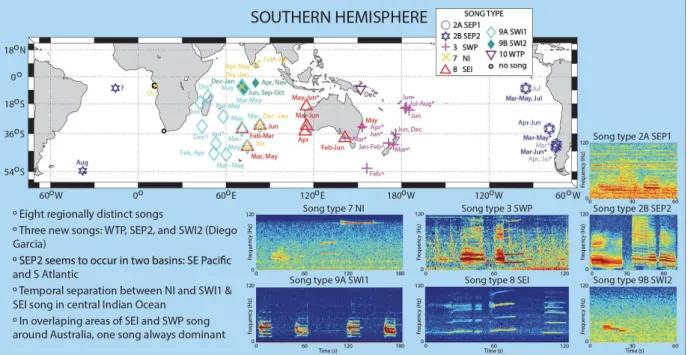
As a result of this pioneering work, there is a global recognition in the biology community of the usefulness ofPAMfor studying cetaceans in their natural environment. In addition, the work summed-up inMcDonald et al.(2006) and, updated as a worldwide collaborative effort inŠirovi´c et al.(2017) (Figure1.4) underlines bio-geographic differences inBWspecies sounds allowing species recognition from anyPAMrecording.

Figure 1.4: Blue whale song diversity, distribution and representation in the Southern hemisphere (Širovi´c et al.,2017).

As heat, light and other forms of electromagnetic energy are severely attenuated in the wa-ter, acoustics is thus the most effective method for marine mammals and whales to perform the various functions associated with their life cycle. Consequently, eavesdropping provides

(36)

unequaled insights into their underwater activities without interfering at all with their natural behavior. When animals are vocally active, the study of their sounds can favor the estimation of their location, of their movements and even, at a broader scale, help into assessing seasonal distributions and density. In addition and, unlike sighting techniques,PAMis not dependent (much) on the weather or brightness, it can provide and record information all day long and all year round, in various contexts, from open waters to beneath the ice, from coastal to remote areas.

Specifically,BWsproduce high intensity and low-frequency vocalizations, probably for long-range acoustic signaling (Payne and Webb,1971). Their specific signatures can exceed a 100 km range (Payne and Webb,1971;Frank and Ferris,2011). These extraordinary vocal abilities are a bargain forPAM: large areas can be monitored with a single sensor.

The tremendous strengths of combiningPAMwith modern unmanned autonomous systems are unequivocal. The ocean and, therefore, marine mammals can now be acoustically monitored over long time scales. As rightfully said byZimmer(2011), in an introduction to his book Passive Acoustic Monitoring of Cetaceans: "As an interdisciplinary subject, successfulPAMcombines physics, technology, and biology ". The relationship between these three topics is discussed throughout this chapter. Primarily, an overview typicalPAMequipment is given in section1.2.

1.2 Passive acoustic monitoring equipment

As there are multiple ways to conduct visual surveys of marine mammals, there are also multiple methods and equipment forPAM(Figure1.5).

Sound speed proﬁle Ocean Bottom Seismometer SOFAR Moored hydrophone Oceanic Glider Tag Sonobuoy

(37)

Hydrophones are the simplest ofPAMsystems. Lowering a single hydrophone in the water from a boat is the easiest way to listen to whales and dolphins. Easy to implement this approach requires minimal hardware and software. It can be improved by the use of multiple hydrophones such as towed arrays, to ease localization and tracking, and contribute to cover larger areas. These types of "dropped-hydrophone(s)" surveys, efficient in coastal areas are not adapted toBWsurveys in remote locations where autonomous systems are preferred. In addition, the low-frequency noise from the towing ship severely limits the detection range, and is the reason why they are rarely used forPAMofBW. The following section gives a brief but non-exhaustive summary of common autonomous instrumentation used today forPAM. A complete review of existing fixed autonomous systems forPAMis presented inNorris et al.(2010) and, a - more recent- full review of real-time instrumentation forPAMis the subject of Baumgartner et al.

(2018).

1.2.1 Autonomous fixed recorders

Fixed (moored) and autonomousPAMinstallations allow for cost-effective long-term monitoring of delimited areas, for extended intervals (e.g., months - years – decades). They are usually separated into two groups depending on the location of the hydrophone in the water column: sound channel-moored hydrophones and bottom-moored hydrophones. When close to shore either systems can be cabled for real-time analysis, overcoming any data storage or limited power supply limits (Ward et al.,2017;Hendricks et al.,2018;Baumgartner et al.,2019).

1.2.1.1 Bottom-moored hydrophones

According toNorris et al.(2010), the first autonomous recorders widely deployed across oceans

wereocean bottom seismometers (OBSs). These instruments, typically equipped with a

seis-mometer, a data logger and batteries to power the device (and later an omnidirectional hy-drophone) were sunk to the seafloor. Data was processed after recovery.OBSsare usually set to have a maximum sampling rate of 100 Hz.McDonald et al.(1995) was the first to useOBSsfor

PAMof blue and fin whales.

Yet,OBSswere too expensive to be purchased and deployed byPAMresearch teams in large quantities and, most bioacoustics team developed their own equipment. Nowadays there is a wide variety of bottom-mounted (or moored) hydrophones covering various frequency ranges such as Cornell Marine Autonomous Recording Units (MARUs - 2 Hz–30 kHz frequency response) (Williams et al.,2014), Rockhoppers1or Scripps HARPs (High-frequency Acoustic Recording Package)2(Širovi´c et al.,2004,2007).

Collaborations between the bioacoustics and geophysical scientific communities expanded the possibility of usingOBSsforPAMof baleen whales e.g.,Dunn and Hernandez(2009);Frank

1_{http://www.birds.cornell.edu/brp/rockhopper/}

(38)

and Ferris(2011); Harris et al.(2013); Brodie and Dunn(2015); Dréo et al.(2019). Table 1.1

presents typicalOBSscharacteristics.

Autonomy 8 month to a year depending on the sampling frequency

Depth maximum 6000 m

Frequency [0 − 50] Hz

Table 1.1: Example of the RHUM-RUMOBScharacteristics (Stähler et al.,2016).

1.2.1.2 Sound channel-moored hydrophones

The deep sound channel is typical of mid-latitude oceans. Physically, in the upper part of the water column, the speed of sound diminishes as the temperature drops. Around depths of 1000 m, when the temperature is constant, the sound speed increases with the hydrostatic pressure (§1.4.2). This inflection point provides a well-defined minimum of celerity and, if an acoustic source is placed at the depth of this minimum, the sound will be "trapped" in this low sound speed layer due to the effect of refraction. The sound can then travel very long distances with little attenuation. This property of theSOFAR, discovered by Ewing and Worzel (Worzel et al.,1948), was showed to be applicable to cross-ocean sound propagation by the Heard island experiment (Munk et al.,1994) using a signal near 57 Hz. For that reason, many recorders are positioned in theSOFARchannel, for example as moored hydrophones floating in the water column, e.g., Southwest of Australia (Gavrilov et al.,2011;Gavrilov and McCauley,2013;Ward et al.,2017) or in the Western Indian Ocean (Samaran et al.,2013;Leroy et al.,2016,2018) (their characteristics are presented on Table1.2).

Autonomy 1 to 2 years

Depth between 500 and 1500 m Frequency [0 − 120] Hz

Table 1.2: Example of the OHASIS-BIO (Observatory in the Indian Ocean) network sound-channel hy-drophones characteristics (Leroy et al.,2018).

1.2.2 Autonomous moving recorders

Autonomous moving recorders are efficient to acquire short term data. Because they do not often require large scientific vessels to be launched, they can be deployed in areas where access is difficult. Moreover, when launched or retrieved, they can be combined with other non-acoustic techniques such as visual observations (or even bio sampling) for multi-approaches monitoring. Contrary to moored devices, they can provide information as thy move, covering a vast perimeter or by monitoring a specific individual.

(39)

1.2.2.1 Sonobuoys

Initially used for military purposes, sonobuoys are one of the most common equipment in the family of acoustic buoy systems forPAMactivities (Clark et al.,1986;Miller et al.,2013). The concept is simple: they relay the sound received by a single hydrophone via a radio signal to a nearby receiver (shipboard or airboard surveys). The additional integration of an orthogo-nally oriented pressure vector sensor and a magnetic compass allows the DIFAR (Directional Frequency Analysis and Ranging) sonobuoy to estimate bearing angles of a sound of interest. A method to estimate the drift direction and speed of a directional sonobuoy is presented inMiller et al.(2018). Cross bearings of two or more sonobuoys allow real-time tracking of target species (Miller et al.,2016;Garcia-Rojas et al.,2018). When batteries run out, the sonobuoy sinks to the bottom of the ocean, in that sense they are disposable equipment. An example of technical sheet is given in Table1.3.

Autonomy between 30 min and 8 hours Depth between 30 and 300 m

Frequency calibrated omnidirectional hydrophone [5 − 20k] Hz DIFAR [5 − 2.4k] Hz

Table 1.3: Example of the 53-F DIFAR sonobuoys characteristics (Rankin et al.,2019).

1.2.2.2 Gliders

In the early 2000, there was a revolution in ocean science: the advent of autonomous underwater vehicles.PAMwas not left behind with, in the summer 2006, the first successful deployment of broadband (5 Hz to 30 kHz) omnidirectional hydrophone seaglider. It recorded calls fromBWs

and humpback whales as well as odontocete sounds (Moore et al.,2007).

Underwater gliders are cost-effective buoyancy-driven vehicles moving vertically up and down in such a way that, at the same time, they gain horizontal distance. They produce almost no self-noise and minimal low-frequency flow noise (Baumgartner et al.,2018). Thanks to con-tinuous efforts and development, they can now be used for real-time monitoring (Baumgartner et al.,2013), and be deployed in previously inaccessible locations such as the Mariana Trench where baleen whale calls were recently recorded (Nieukirk et al.,2016). The characteristics of the glider used in this experiment are presented in Table1.4. Their continuous motion is slow compared to most marine mammals movements. Moreover, they can offer good spatial coverage in comparison to fixed sensors and are easier to deploy. These features are the reason why gliders are progressively considered for classical conservation applications such as animal density estimation (Marques et al.,2013).

(40)

Autonomy Technically almost unlimited, virtually months Depth between 0 and 1000 m

Frequency between 15 Hz and 97 kHz

Table 1.4: Example of the Seaglider™ characteristics (Nieukirk et al.,2016).

1.2.2.3 Bio-logging or TAGs

Bio-logging or more commonly "tagging" consists in deploying a high-resolution multi-sensor device directly on an individual in order to document a portion of its life. In addition to the hydrophone, acoustic tags can be equipped with a hydrostatic pressure sensor (depth), an accelerometer, a temperature sensor and, a compass (see models Acousondes3and Dtags4). Some of these devices can also be equipped with a radio antenna for communication. These methods are designed to be non-invasive, e.g., fixed using suction pads in order to satisfy modern ethical standards and least affect animal behavior.

Figure 1.6: Ari Friedlaender deploys a multi-sensor suction cup tag on a humpback whale in Antarctica’s Wilhelmina Bay (Photo by Ari Friedlaender, source:https://www.bates.edu/).

Because they require contact with the whale (Figure1.6), they are often combined with skin samples for sex or DNA determination. Acoustic tags have provided information on call types, call frequencies, cue production rates, seasonality and sex differences in vocalizations forBWs

(Stimpert et al.,2015). More recently, thanks to their combination with different sensors, tags have been used to estimate the depth(s) at whichBWsing, evaluated about 30 m (Lewis et al.,

2018). Characteristics of the DTAG3 used inStimpert et al.(2015) is presented on Table1.5. 3_{http://www.acousonde.com}

(41)

Autonomy up to 3 days depending on the sampling frequency Depth 500 to 3000 m

Frequency between 10 Hz and 20 kHz

Table 1.5: Example of the DTAG3 characteristics (Stimpert et al.,2015).

1.2.3 Discussion

Table1.6summarizes all the presented visual and acoustic survey methods and, compares their ability to conduct continuous surveys, display common time-scales, if they are communicating and if they can identify an individual or a species. Unique sensors are considered, and tracking opportunities are not yet discussed. In comparison to sightings,PAMoffers continuous and

Method Continuous Duration Real-time Identiﬁcation hours day months year Individual species Sightings Visual survey Aerial surveys Drone Satellite imagery

PAM _{Auto. ﬁxed}

recorders

Sono buoy

Glider

TAG

Table 1.6: Baleen whale survey methods recap: white = no, blue = yes and gray = maybe.

multi-time scale opportunities to surveyBWswithout intruding their environment. However, Table 1.6 also shows that, because sounds are subspecies-specific, it is impossible to use a unique omnidirectional sensor to identify individuals within a species. Besides, to identify new species-sound connections, cross-referencing with, e.g., visual observations or known migration patterns, is essential. This is why all the methods above are complementary, to learn about, survey, and protect efficiently marine mammals using information based multiple time, space, and resolution scales (Nowacek et al.,2016). A brief overview ofPAMfall on for animal ecology is given in section1.3.

(42)

1.3 Applications of passive acoustic monitoring

The first and most direct application ofPAMis to study animal sounds as part of their com-munication. Call and song description, as well as the identification of new signatures (Leroy et al.,2017a;Ward et al.,2017), can help to identify connected species or subspecies (McDonald et al., 2006) and, identify vocally active populations (Balcazar et al.,2015;Brodie and Dunn,

2015). Additional information on source levels (Cummings and Thompson,1971;Samaran et al.,

2010c;Širovi´c et al.,2007;Weirathmueller et al.,2013) intervene in the understanding one can have on sound production mechanisms (Adam et al.,2013;Cazau et al.,2016;Adam et al.,2018). Tagging equipment permits the observation and sampling of individual behavior (Lewis et al.,

2018). The study of song structure and their variations recently showed gradual synchronization and modification of song rhythms for two Californian fin whales populations over long time scales, indicating some exchanges or visitation among populations (Širovi´c et al.,2017). More recentlyJolliffe et al.(2019) demonstrated an increase in song diversity of pygmyBWs, consistent with cultural evolution but, the consequence of (yet) unknown factors. Thorough call analysis also revealed, in addition to seasonal frequency variation, a constant decline of large whale call frequencies over the last decade (McDonald et al.,2009;Leroy et al.,2018) but explanations are yet to be found.

Based on call analyses and pattern recognition algorithms,PAM can be used in animal ecology (Zimmer,2011):

· to estimate the abundance, the total number of animals in a given area or, equivalently, a population density of the species of interest;

· to mitigate the impact of anthropogenic activity on marine mammals or, to estimate cetacean presence/absence, necessary for risk mitigation.

Note that the method employed for ecology analyses depend on the number of sensors (mono-sensor or multi-(mono-sensor), their type (omnidirectional or vectorial) and their spatial distribution. Some configurations enable to localize, track and differentiate individuals.

Habitat analysis is based on the idea that whales are not uniformly distributed throughout the world and that their distribution shows spatial and temporal heterogeneity (Zimmer,2011).

PAMcan therefore be used to determine whale-inhabited waters and identify the populations (Delarue et al.,2009;Samaran et al.,2010b;Cerchio et al.,2015;Garcia-Rojas et al.,2018). It can help draw geographical and seasonal patterns across vast areas (Širovi´c et al.,2004;Stafford et al.,2011;Tripovich et al.,2015;Leroy,2017), refine known migratory corridors (Thomisch,

2017) and, identify and locate species-specific feeding and breeding grounds (Gedamke et al.,

2007;Samaran et al.,2013). A better knowledge of whale territories is essential for conservation purposes, as a first step before taking measures on the management of specific areas, for example, to mitigate ship strikes and entanglements (Irvine et al.,2014;Harcourt et al.,2019).

(43)

Last but not least,PAMcan help to evaluate whale response to global anthropogenic noise (Melcon et al.,2012). Indeed, anthropogenic noise has the potential to mask whale communi-cation and therefore, to limit their communicommuni-cation range. It has serious consequences since, according toWilliams et al.(2014), acoustic masking is "a qualitatively similar stressor to habitat loss." For instance, ship traffic can directly affect whale acoustic environment (Redfern et al.,

2017) and have been seen to cut down by 87% the communication space of Bryde’s whales on routine passages (Putland et al.,2018). The study of transient sounds repercussion on marine life also demonstrated the disturbance ofBWsbehavior under the effect of mid-frequency military

sonar(Goldbogen et al.,2013;Harris et al.,2018). However, the effect of noise on animals and

the in-place regulations are controversial subject (Gomez et al.,2016).

To efficiently monitor blue whales, knowledge of fundamental underwater acoustic propa-gation is essential, for all intended applications. Physical properties such as the spreading of the acoustic wave energy or attenuation need to be taken into account in the estimate ofPAM

system detection ranges. Underwater acoustics key elements are thus discussed in Section1.4.

1.4 Underwater acoustics

1.4.1 Geometrical or Modal propagation?

The wave equation showing the relationship between the spatial and temporal variations of the acoustic pressure p is given by

∇2p − 1 c2

∂2p

∂t2 = 0, (1.1)

where c represents the speed of sound and where the spatial differences are described by the Laplacian operator ∇2, the form of which depends in the coordinate system chosen for the application.

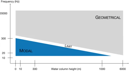
In underwater acoustics, as presented in Figure1.7, there are two approaches to understand and integrate propagation in models as well as in the interpretation of observations: the geo-metrical and the modal approach. The geogeo-metrical approach is generally considered as a "high frequency" approximation derived from the eikonal equation. Under these assumptions the acoustic wavefront is represented by a finite number of rays, each one following their trajectory depending on the position of the source, the emission angle(s), and the sound speed (Urick,

1983). However, other solving methods exist. For example, the modal approach requires an accurate resolution of the acoustic pressure field (same order as the wavelength) and is therefore generally considered as a low-frequency approach.

In underwater acoustics, the modal approach is generally considered when the wavelength and the characteristic dimension (the water column height, H) are of the same order: it considers the standing waves over the vertical ocean. When consideringBWsounds in the deep ocean, the maximum wavelength of their sounds in the order of 150 m (c = 1500 (m/s) and f = 10 Hz)

(44)

300 20 10 0 10 300 1000 6000 20000

G

EOMETRICAL

M

ODAL LIMIT Frequency (Hz)

Water column height (m)

Figure 1.7: Range of validity of modal and geometrical propagation as a function of frequency and watercolumn height (adapted fromJosso(2010)).

is more than 20 time smaller than average ocean depth ≃ 3500 m. Under these considerations, geometrical assumptions are used in this study to model the propagation ofBWsounds.

1.4.2 Sound speed profile and refraction

1.4.2.1 Sound speed profile

Depth (m ) Sound speed c(z) (m/s) 0 500 1000 1500 1500 1520 1480 Surface Layer Main Thermocline

Deep Isothermal Layer Temperature  

variations

Hydrostatic   pressure

Figure 1.8: Sound speed profile and influential parameters (adapted fromUrick(1983)).

(45)

the fact that the sound speed is not constant. In general, c is determined by a complex rela-tionship between salinity, temperature, and hydrostatic pressure, the last two being the most influential. In a specific area, it mostly varies with depth (therefore denoted c(z)), showing a stratification of the ocean (Urick, 1983). An example of typical mid-latitudes deep-ocean profile is depicted in Figure1.8, showing the two principal characteristics of the sound speed profile: the thermocline where c(z) drops with the temperature and, the isothermal layer, where c(z) increases with the hydrostatic pressure. Variations in surface temperature (due to latitude, seasonal changes or weather) change the sound speed profile.

1.4.2.2 Refraction and the Snell’s law

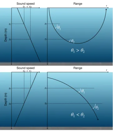
The stratification of the ocean (in depth) induced by variations in the water column parameters and, especially sound speed variations, has an effect on the propagation of the acoustic wave: it is subject to refraction. Acoustic rays are deviated according to the Snell’s law

cosθ1

c1 = cosθ2

c2 , (1.2)

where indices 1 and 2 correspond to two different depths in the water column with z1< z2, and θ represents the grazing angle (Figure1.9). Then considering a simple sound speed profile,

· if c1< c2, the grazing angle diminishes (θ2< θ1) until total refraction and, the ray bends towards the surface, to the minimum sound-speed,

· if c1> c2, the grazing angle increases (θ2> θ1) and, the ray bends towards the ocean floor, again to the minimum sound-speed.

Depth (m ) Sound speed c1 c2 z1 z2 r z1 z2 θ₂ Range < θ₁> θ₂ θ₁ Depth (m ) Sound speed c2 c1 z1 z2 r z1 z2 θ 1 θ 2 Range θ 1< θ2 <

(46)

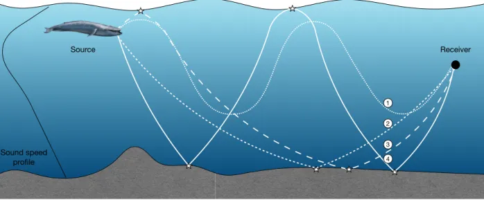
In other words, the geometrical model of the underwater acoustic propagation is a complex model where, acoustic beams do not propagate in straight lines but, bend towards the minimum sound speed under the effect of refraction. They can reflect at the surface and bottom boundaries, as illustrated in Figure1.10. Consequently, a receiver can record rays that traveled different paths: direct or with bottom and surface reflection(s). At low frequencies, the sea surface can be seen as a perfect screen where the acoustic wave reflects with only a phase change. However, some energy might be transmitted into the seafloor, depending on the nature of the material.

Sound speed proﬁle Source Receiver 1 2 3 4

Figure 1.10: Illustration of different acoustic paths: (1) Direct, (2) one bottom reflection (3) one bottom and one surface reflections and, (4) two bottom and one surface reflections.

In order to carry out numerical simulations of the propagation, numerous software have been developed, the most popular being Bellhop (Porter and Bucker,1987). This program, developed by Porter in the 1980s is freely available online5. An example of propagation with a source placed at a 30 m depth and a statistical deep ocean sound-speed profile for the Indian Ocean in May is presented in Figure1.11. Acoustic rays fill the entire water column with multiple bottom-surface reflections. Ray tracing illustrates 2D propagation space coverage, but, the analysis can be completed with energetic considerations.

Figure 1.11: Propagation simulation, source depth zs= 30 m, θ = [−20;45]°, propagation range r = 100 km.