HAL Id: hal-00919434
https://hal.archives-ouvertes.fr/hal-00919434
Submitted on 16 Dec 2013
HAL is a multi-disciplinary open access
archive for the deposit and dissemination of
sci-entific research documents, whether they are
pub-lished or not. The documents may come from
teaching and research institutions in France or
abroad, or from public or private research centers.
L’archive ouverte pluridisciplinaire HAL, est
destinée au dépôt et à la diffusion de documents
scientifiques de niveau recherche, publiés ou non,
émanant des établissements d’enseignement et de
recherche français ou étrangers, des laboratoires
publics ou privés.
Predictability Analysis of Distributed Discrete Event
Systems
Lina Ye, Philippe Dague, Farid Nouioua
To cite this version:
Lina Ye, Philippe Dague, Farid Nouioua. Predictability Analysis of Distributed Discrete Event
Sys-tems. 52nd IEEE Conference on Decision and Control, Dec 2013, Florence, Italy. pp.5009-5015.
�hal-00919434�
Predictability Analysis of Distributed Discrete Event Systems
Lina Ye and Philippe Dague and Farid Nouioua
Abstract— Predictability is an important system property that determines with certainty the future occurrence of a fault based on a model of the system and a sequence of observations. The existing works dealt with predictability analysis of discrete-event systems in the centralized way. To deal with this important problem in a more efficient way, in this paper, we first propose a new centralized polynomial algorithm, which is inspired from twin plant method for diagnosability checking and more importantly, is adaptable to a distributed framework. Then we show how to extend this algorithm to a distributed one, based on local structure. We first obtain the original predictability information from the faulty component, and then check its consistency in the whole system to decide predictability from a global point of view. In this way, we avoid constructing global structure and thus greatly reduce the search space.
I. INTRODUCTION
Fault diagnosis is a crucial and challenging task in the au-tomatic control of complex systems ([12] , [11], [1]), whose efficiency depends on a system property called diagnosabil-ity. The diagnosability problem has received considerable attention in the literature. The existing works analyzed diag-nosability both in the centralized way and the distributed way ([9], [6], [3], [8], [10]). However, diagnosability concerns the system ability to determine whether the fault has effectively occurred based on the observations. Sometimes it is very expensive to recover the system after fault occurrence, which motivates the work on the analysis of system ability to predict with certainty future faults based on the observations from the system whose current state is normal.
Predictability is a crucial system property that determines at design stage whether the considered fault can be correctly predicted before its occurrence based on available observa-tions. If the fault is predicted, the system operator can be warned and may decide to halt the system or otherwise take preventive measures. However, up to now, only few works have dealt with this subject in the domain of diagnosis for discrete event systems. The authors of [4] proposed a deterministic diagnoser approach in a centralized way, which has exponential complexity with the number of system states. Then in [5], a polynomial approach was presented but only in a centralized way.
In this paper, we propose a new efficient polynomial al-gorithm for predictability analysis of discrete event systems,
L. Ye is with INRIA Grenoble (The National Institute for Research in Computer Science and Control), 655, avenue de l’Europe, Montbonnot, F-38334 Saint Ismier Cedex, [email protected]
P. Dague is with the Laboratory of computer science (LRI), Univ. Paris-Sud & CNRS, Bˆat 650, 91405 Orsay Cedex, France [email protected]
F. Nouioua is with the Department of computer science, University of Aix-Marseille, Avenue Escadrille Normandie-Niemen, 13397 Marseille Cedex 20, [email protected]
which is, more importantly, well adaptable to a distributed framework. First, we show how to construct an essential structure called pre twin plant, inspired from twin plant method for diagnosability analysis, based on which pre-dictability is analyzed by checking the existence of special states that violate predictability definition. Then we give and prove a sufficient and necessary condition for predictability that can be checked algorithmically. The most important contribution of this paper is the extension of this algorithm to a distributed way. The idea is to obtain the original pre-dictability information from the faulty component and then to check its global consistency to decide global predictability. In this way, we avoid constructing global structure and thus greatly reduce search space.
The rest of the paper is organized as follows. The next sec-tion presents the system model and recalls the predictability of discrete event systems. Section 3 proposes a polynomial algorithm for predictability in a centralized way before extending it to a distributed framework in Section 4. Then we conclude in Section 5.
II. PRELIMINARIES
A. System Model
We model a discrete event system as a Finite State
Machine (FSM), denoted by G = (Q, Σ, δ, q0), where Q
is the set of states, Σ is the set of events, δ⊆ Q × Σ × Q is the set of transitions (the same notation will be kept for its natural extension to words of Σ∗) and q0 is the initial state. The set of events Σ is divided into three disjoint parts: Σothe
set of observable events, Σu the set of unobservable normal
events and Σfthe set of unobservable fault events. Given two
FSMs G1 and G2, their synchronization, denoted by G1∥G2,
is based on the set of shared events. Only the shared events are synchronized events that should occur simultaneously while the private events can occur independently whenever possible. It is easy to generalize this for a set of FSMs using the associativity properties [2].
Example 1: Figure 1 shows an example of system model, where observable events are denoted by Oi, unobservable normal events by U i, unobservable fault event by F .
O1 O2 X1 X2 F X4 U1 X0 X3 O1 O3 X5 X6 X8 O2 X7 O1 O3 O1 O2
Given a system model G, its prefix-closed language L(G), which describes both normal and faulty behaviors of the system, is a subset of the Kleene closure of Σ: L(G)⊆ Σ∗. Formally, L(G) is the set of words produced by G: L(G) =
{s ∈ Σ∗|∃q ∈ Q, (q0, s, q)∈ δ}. In the following, we call a word from L(G) a trajectory in the system G and a sequence
q0σ0q1σ1... a path in G, where σ0σ1... is a trajectory in G and for all i, we have (qi, σi, qi+1) ∈ δ. Given s ∈ L(G),
we denote the post-language of L(G) after s by L(G)/s,
formally defined as: L(G)/s ={t ∈ Σ∗|s.t ∈ L(G)}. The
projection of the trajectory s to observable events of G (resp.
Gi in distributed systems) is denoted by P (s) (resp. Pi(s)).
We assume that the system language is always live.
B. Predictability for Discrete Event Systems
Predictability is considered as a crucial property of a system since a fault can possibly be avoided when it is predictable. As diagnosability analysis, our predictability algorithm has exponential complexity with the number of faults (see Section IV-C for more details). To reduce the complexity, we consider fault one by one separately, which is also the case in the extended distributed algorithm. We rephrase the predictability definition as follows [4]. Here a trajectory ending with a fault F is denoted by sF, the set
of prefixes of the trajectory sF is denoted by sF, and N
represents the set of natural numbers.
Definition 1: (Predictability). A fault F is predictable in
a system G iff
(∀sF ∈ L(G))(∃k ∈ N)(∃t ∈ sF)[(F /∈ t) ∧ D]
where D : (∀p ∈ L(G)) (∀p′ ∈ L(G)/p)
[(P (p) = P (t))∧ (F /∈ p) ∧ (∥p′∥ ≥ k) ⇒ (F ∈ p′)].
The above definition implies that a fault F is predictable iff for any trajectory ending with the fault sF, there exists at least one prefix of sF, denoted by t, such that t does not contain F and for each non faulty trajectory p with the same observations as t, all the long enough continuations of p should contain F . Only in this way, F can be certainly pre-dicted before its occurrence based on the same observations as those in t.
III. CENTRALIZED ALGORITHM
Now we recall the twin plant method, initially used for diagnosability analysis, and then show how to adapt it to analyze predictability. The idea of twin plant is to construct a structure that obtains all pairs of trajectories with the same observations [6], which is based on another structure called
diagnoser built from system model 1. A diagnoser provides
the information about fault occurrence in each state of the system.
Definition 2: (Diagnoser). Given a system model G,
its diagnoser is the nondeterministic FSM D =
(QD, ΣD, δD, qD0), where QD ⊆ Q × {N, F } is the set of
states, ΣD= Σ is the set of events, δD⊆ QD× ΣD× QD
1To be consistent with the distributed method developed later, we follow
the diagnoser, twin plant introduced in [6] except keeping observable events as well as non-observable events, the latter will be used in predictability analysis in distributed framework, this is also the case for pre twin plant.
is the set of transitions, and qD0 = (q0, N ) is the initial
state of the diagnoser. The transitions of δD are those
((q, l), e, (q′, l′)) with e ∈ ΣD, (q, l) reachable from the
initial state qD0, (q, e, q′) ∈ δ and satisfying the following conditions:
• if l = F , then l′ = F ;
• if l̸= F and e = F , then l′ = F ;
• if l̸= F and e ̸= F , then l′ = N.
In a diagnoser, we add fault label F to the states, up to which the fault has effectively occurred, and normal label
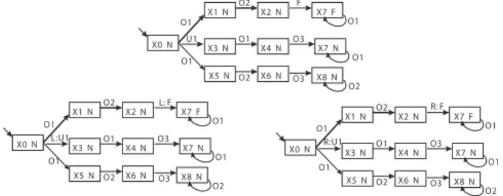
N to those without the fault occurrence. The top part of
Figure 2 shows the diagnoser for the system of Example 1. Given a diagnoser, its corresponding twin plant is obtained by synchronizing this diagnoser with itself, called left and right instances (denoted by Dl and Dr, respectively), based
on the set of observable events. From Definition 2, we know that a diagnoser keeps all system events. However, to build the twin plant, only observable events should be synchronized to obtain all pairs of trajectories with the same observations. To do this, all other non observable events are distinguished between the left instance and the right instance by the prefixes L and R respectively. In the following, we use
AddP re(G, Str, Σ) to denote the addition of the prefix Str
to all events contained in Σ of the FSM G. Thus, we have
Dl = AddP re(D, L:, Σ′) and Dr = AddP re(D, R:, Σ′),
where Σ′ is the set of non observable events, i.e., Σ′ =
Σ\Σo. The bottom part of Figure 2 shows the left instance
and the right instance of the diagnoser, respectively. Now we
X0 N X1 N X2 N X5 N O1 O2 X6 N O2 O1 O1 X7 F F O2 X8 N X3 N X4 N O1 O1 X7 N O3 U1 O3 X0 N X1 N X2 N X5 N O1 O2 X6 N O2 O1 O1 X7 F O2 X8 N X3 N X4 N O1 O1 X7 N O3 R:U1 O3 X0 N X1 N X2 N X5 N O1 O2 X6 N O2 O1 O1 X7 F L: F O2 X8 N X3 N X4 N O1 O1 X7 N O3 L:U1 O3 R: F
Fig. 2. Diagnoser D (top), left instance Dl(bottom left) and right instance
Dr(bottom right).
rephrase the definition of twin plant [6], as follows.
Definition 3: (Twin Plant). Given a diagnoser D, the
corresponding twin plant is obtained by synchronizing its left instance with its right instance based on the set of observable events, denoted by T = (QT, ΣT, δT, q0T) = Dl∥Dr.
In a twin plant T , each state is composed of a pair of diagnoser states providing two possible diagnoses with the same observations. Given a twin plant state ((ql, ll), (qr, lr)),
if ll = lr = N , this state is called a normal state. If
ll= lr= F , it is called a faulty state. Otherwise, if ll̸= lr,
it is called an uncertain state.
Recall that a fault is diagnosable iff we can be sure that the fault has effectively occurred based on long enough sequence of observations after the fault occurrence [9]. In other words, the existence of two indistinguishable behaviors, i.e., holding the same enough observations with exactly one
of them containing the given fault, violates the diagnosability property. The diagnosability analysis is therefore to check the existence of such behaviors. Thus, the twin plant defined as above is sufficient for diagnosability checking since for each path, the corresponding two trajectories always have the same observations, from the beginning to the end. A path with an uncertain cycle in the twin plant corresponds to two indistinguishable behaviors. While for predictability analysis, we check whether the future occurrence of the fault can certainly be predicted based on the observations of a trajectory not yet containing the fault. In other words, we should compare the observations of two trajectories only before the fault occurrence and do not care about whether they have the same observations after the fault, i.e., synchronized events are only observable ones before the fault. Before proposing pre twin plant, we first define the union of two FSMs such that one FSM can be combined to the other as its continuation, i.e., the initial state of one FSM is contained in the state space of the other FSM. This will be used in constructing pre twin plant.
Definition 4: (Union of FSMs). Given two FSMs G1 = (Q1, Σ1, δ1, q01) and G2= (Q2, Σ2, δ2, q20), then their union is G1∪ G2 = (Q1∪ Q2, Σ1∪ Σ2, δ1∪ δ2, q0), where the initial state of the union q0 is defined as follows:
• if q10∈ Q2, then q0= q02
• if q20∈ Q1, then q0= q01
We do not consider the case where q0
1 ∈ Q/ 2∧ q02 ∈ Q/ 1 or
q0
1 ∈ Q2∧ q20 ∈ Q1∧ q01 ̸= q20. The former means that the two FSMs are totally independent in terms of state and thus cannot be unified. In the latter case, there is no initial state after the union since both initial states in the two FSMs after the union have at least one input transition.
Now, we construct pre twin plant for predictability in the following way, which is to obtain all pairs of trajectories with the same observations before the occurrence of the fault if there is any.
Definition 5: (Pre Twin Plant). Given the left instance and
the right instance of a diagnoser, Dland Dr, the
correspond-ing pre twin plant, denoted by Tp = (Q
Tp, ΣTp, δTp, q0Tp), is obtained by the following steps.
1) Tp = Dl∥
SFD
r, where ∥
SF is a special
synchro-nization that stops each time when the state becomes non-normal state for the first time, i.e., after the first occurrence of the fault.
2) ∀(qTp, F, q′Tp) ∈ δTp, if qTp = (qDl, qDr) is a normal state, we perform T emAddP re(Dl, L:, ΣqDl
o ), T emAddP re(Dr, R:, ΣqDr o ) and Tp = Tp ∪ (Dl:q Dl∥Dr:qDr), where Σ qDl
o (ΣqoDr) denotes the set
of observable events in Dl (Dr) reachable from q
Dl (qDr) and Dl:qDl (Dr:qDr) is the part of Dl (Dr) that begins from the state qDl (qDr).
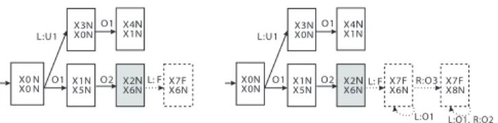
Step 1 is to synchronize the left and right instances of the diagnoser based on the set of observable events, which should stop whenever the state switches from normal state to non-normal one. This is illustrated by the left part of Figure 3. Since for predictability, we do not care about whether the observations of two trajectories after the fault
are the same or not, in step 2, we distinguish the observable events after the first fault occurrence by using the function
T emAddP re(G, Str, Σ), which is to temporarily add the
prefix Str to all events in Σ of the FSM G. Here what we mean by temporarily is that the addition of a prefix is only valid during step 2 when dealing with one normal state immediately before the fault. In other words, if we go on to treat another normal state before the fault, we use the original instances without such prefixes. The reason is that the same observable event may occur before the fault in one path while after the fault in another path. In the pre twin plant, the normal part, i.e., part before fault, is called Obs-Equivalent (OE) part since the corresponding trajectories have the same observations and the non-normal part, i.e., part since fault, is called Non-Obs-Equivalent (NOE) part, where observable events are not synchronized events any more. Intuitively, each path in the pre twin plant corresponds to a pair of trajectories that have the same observations before fault occurrence. For predictability analysis, what we are interested in is those normal states that are within unobservable reach such that an immediate successor is a non-normal state. Now we define such states, which draw the boundary from normal states to non-normal ones.
Definition 6: (Critical Normal State). Given a pre twin
plant Tp, the set of critical normal states, denoted by Γ c,
is defined as Γc = {qc ∈ QTp|qc is normal and ∃q ∈
QTp, (qc, su.F, q)∈ δTp, where su∈ Σ∗u}.
Before critical normal states, we have the same observations for the corresponding pair of trajectories. The right part of Figure 3 illustrates a part of the pre twin plant for the system of Example 1. Here we use dashed arrows to represent the transitions in the NOE part and normal arrows for those in the OE part. The nodes with dashed frame represent uncertain states. The gray node ((X2N )(X6N )) is a critical normal state since it is a normal state immediately before the first occurrence of the fault. Note that from this critical normal state, there is a reachable uncertain cycle containing events both from the left and right instances. This means that the corresponding pair of infinite trajectories have the same observations before the fault and only one of them contains the fault, which violates predictability.
X3N X0N L:U1 X0N X0N X4 X1NN O1 O2 X7F X6 N X7F X8N R:O3
L:O1 L:O1, R:O2 X1N X5N O1 X2 X6NN X3N X0N L:U1 X0 N X0 N X4 X1NN O1 O2 X7F X6N L: F X1N X5N O1 X2 X6NN L: F
Fig. 3. Part of FSM obtained from step 1 of Definition 5 for system in Example 1 (left) and part of its pre twin plant (right).
Theorem 7: A fault is predictable in the system iff in the
corresponding pre twin plant, there is no critical normal state
qcsuch that there exists at least one uncertain cycle reachable
from qc containing at least one event from the left instance
Proof:
(⇒) Suppose that a given fault F is predictable and that there does exist a critical normal state qc in the pre twin
plant, from which we have one reachable uncertain cycle, denoted by ϕ, that contains events both from the left instance and the right instance. Now we denote the pair of trajectories corresponding to the path containing qc and ϕ as s and s′,
where one trajectory, suppose s, contains the fault and s′
does not. This is deduced from the fact that ϕ is an uncertain cycle. Since each path in the pre twin plant corresponds to a pair of trajectories with the same observations before fault occurrence, then for the non faulty prefix of s up
to qc, denoted by t, the trajectory s′ must have a non
faulty prefix with the same observations as t, which has
enough continuation without the fault. Considering that qc
is a boundary to switch from normal state to non-normal one, i.e., the prefix up to qc is a normal prefix of s with the
maximum number of observable events, it follows that for each normal prefix t′ of the faulty trajectory s, s′ always has a normal prefix with the same observation as t′ but with enough continuation without the fault, i.e., infinite normal continuation, which violates the predicability definition. This contradicts the assumption that F is predictable.
(⇐) Now suppose that the fault F is not predictable and that there is no critical normal state as described above. From the non predictability of F , we know that there does exist at least one faulty trajectory s with enough events such that for each normal prefix of s, we can always find another non faulty trajectory with the same observations as this normal prefix that has at least one enough continuation without the fault, i.e., infinite normal continuation. Now suppose t is the longest normal prefix of s, after which is the first occurrence of the fault. Then a non faulty trajectory with the same observations as t is denoted by p and one of its infinite normal continuations is denoted by p′. From the way to construct the pre twin plant, we know that the pair of trajectories s (left instance) and p.p′ (right instance) are synchronized as a path in the pre twin plant since they have the same observations before the fault occurrence. It follows that this path should have at least one critical normal state with a reachable uncertain cycle containing both events from the left instance and the right instance since the system language is assumed to be live. This implies that the assumption is contradicted.
Consider Example 1. In the pre twin plant partly shown in Figure 3, we have at least one critical normal state with a reachable uncertain cycle containing events from left and right instances, which, from Theorem 7, implies that the fault is not predictable. More precisely, consider
the faulty trajectory s = (O1.O2.F.O1∗), which has two
normal prefixes p1 = O1 and p2 = O1.O2. We have a
normal trajectory s′ = (O1.O2.O3.O2∗) such that for both
p1 and p2, s′ has a prefix with the same observations as
them but with enough normal continuation. When we obtain the observable events in any normal prefix of s, i.e., O1 or
O1.O2, we can never be sure about the future occurrence of F since both s and s′ have the same observations before F
but only s contains F .
IV. EXTENSION TO DISTRIBUTED FRAMEWORK In this section, we show how to extend our centralized method to a distributed framework. We consider a distributed discrete event system composed of a set of components
G1, ..., Gnthat communicate by communication events. Each
component is modeled by a FSM, denoted by Gi =
(Qi, Σi, δi, qi0), where Qi is the set of states, Σi is the set
of events, δi⊆ Qi× Σi× Qi is the set of transitions and q0i
is the initial state. The set of events Σi is divided into four
disjoint parts: Σio the set of observable events, Σiu the set of unobservable normal events, Σif the set of unobservable fault events and Σicthe set of unobservable communication events shared by at least one other component. For any pair of distinct local components Giand Gj, we have Σio∩Σjo =∅, Σiu ∩ Σju = ∅ and Σif ∩ Σjf = ∅, which means that the only shared events between different components are communication events. Thus, given a considered fault F , it
can only occur in one component, denoted by GF (called
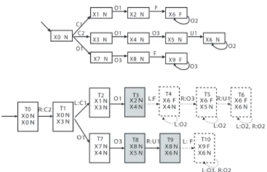
the faulty component, the others being the normal ones). We assume that the language for each component is always live. Example 2: Figure 4 presents a simple distributed system composed of two components, where observable events are denoted by Oi, unobservable normal events by U i, unob-servable fault event by F and unobunob-servable communication events by Ci.
The global model is implicitly defined as the synchronization
of the two components G = G1∥G2, where the synchronized
events are communication events, i.e. shared events.
C1 O1 X1 X2 F X4 C2 X0 X3 O1 C1 Y0 Y1 O4 C2 Y3 Y2 O5 F X7 X8 X9 O3 X6 O2 O6 O3 X5 U1 O1 O3
Fig. 4. A distributed system composed of two components: G1(left) and
G2(right).
A. Original Predictability Information
In the distributed framework, since the fault can only occur in the component GF, to obtain the original predictability
information, we construct the local diagnoser DF for GF
and then the corresponding pre local twin plant TFp, shortly called PLTP, whose constructions are similar to those for centralized approach, i.e., Definition 2 and Definition 5. The only difference is that communication events are handled in the same way as unobservable events. Figure 5 shows
the local diagnoser (top) for the faulty component G1 of
Example 2 and a part of its PLTP (bottom), where the gray nodes represent critical normal states.
B. Global Consistency Checking
Given a PLTP, we obtain the critical normal states in the same way as in the centralized method. However, until now we only consider the faulty component, whose connection to
X0 N X1 N X2 N X7 N C1 O1 X8 N O3 O2 O1 X6 F F O3 X9 F F X3 N X4 N O1 O2 X6 N U1 X5 N O3 C2 X0 N X3 N X7 N X4 N X1 N X3 N O1 L:C1 X0 N X0 N X8 N X5 N X8 N X6 N X2 X4 NN R:C2 O3 R:U1 O1 X6 F X4 N L:F X6 F X5 N R:O3 X6 F X6 N R:U1 L:O2 L:O2 L:O2, R:O2
X9 F X6 N L: F L:O3, R:O2 T0 T1 T2 T3 T4 T5 T6 T7 T8 T9 T10
Fig. 5. Local diagnoser D1 (top) and part of PLTP T1p(bottom) for the
faulty component G1 .
the neighborhood is not yet taken into account. After syn-chronization with other components, the reachable uncertain cycles after critical normal states in the PLTP may disappear or those critical normal states originally without reachable uncertain cycle may later have such ones. So, the next step is to check the global consistency of the PLTP, i.e., checking the existence of critical normal states with reachable uncertain cycles after synchronization. Given a path p1 and a path
p2, if the synchronization of p1 with p2 is blocked at state q = (q1, q2) due to different synchronized events, then we
say (q, p1, p2) is a blocked point, i.e., a blocked state q with respect to p1 and p2. Now we define pre local twin checker for normal components, shortly PLTC, which is used to be synchronized with PLTP for global consistency checking. The idea is similar to PLTP except that there is no fault information for PLTC.
Definition 8: (Pre Local Twin Checker (PLTC)). Given
a normal component Gi, the corresponding pre local twin
checker (PLTC), denoted by Cip, is obtained as follows.
1) The left instance of Gi is obtained by Gli =
AddP re(Gi, L:, Σ′i) and the right instance of Gi is
obtained by Gri = AddP re(Gi, R:, Σ′i), where Σ′i is
the set of non observable events in Gi, i.e., Σ′i =
Σi\Σio. 2) Cip= Gli∥Gri.
3) In Cip, for each blocked point (q, pl, pr),
where q = (ql, qr), pl is in the left instance
and pr is in the right instance, we perform
temporary addition of prefix before continuing
synchronization, i.e., T emAddP re(Gl
i, L:, Σ ql:pl io ), T emAddP re(Gr i, R:, Σ qr:pr io ), and C p i = Cip ∪ ((pl:ql)∥(pr:qr)), where Σql:pl io (Σ qr:pr io ) represents the set of observable events reachable from
ql (qr) in pl (pr) and pl:ql (pr:qr) is the part of pl
(pr) that begins from the state ql (qr).
In PLTC, the part obtained by step 2 is called Obs-Equivalent (OE) part and the other part obtained by step 3 is called Non Obs-Equivalent (NOE) part. We reuse the function
T emAddP re to denote that the temporary addition of prefix
is only valid during the step 3 when dealing with current blocked point. When we continue for other blocked points, we use the original instances without such prefixes
con-sidering that the same observable event can be in the OE part of one path while in the NOE part of another path. Here the reason why we take steps to unblock the parts where observations are different is that we construct PLTCs to synchronize with the PLTP to check the existence of reachable uncertain cycle after critical normal states from a global point of view. In a normal component, for those parts occurring after the fault after synchronization with
GF, we do not care about whether the observations of two
trajectories are the same or not. But during the construction of PLTCs, we do not know which parts are after the fault, thus we unblock all parts as described above. During the synchronization of the PLTP and PLTCs, we will impose a constraint to guarantee the same observations before the fault occurrence, which will be explained later. Part of the PLTC
for the component G2 of Example 2 is depicted in Figure
6, where the transitions in the NOE part are represented by dashed arrows. Here the gray node S1 is a blocked state.
Y2 Y2 O5 Y0 Y0 Y2 Y3 Y1 Y1 R:C2 R:C1 Y1 Y2 R:O5 Y3 Y2 L:O4 Y3 Y3 R:C2 L:O6 L:O6, R:O6 Y1 Y0 L:C1 O4 L:C2 O6 S0 S1 S2 S3 S4 S6 S7 S5
Fig. 6. Part of PLTC for the component G2.
Given the PLTP and a set of PLTCs, whose correspond-ing components are GF, Gk1, ..., Gkm, where Gki, i ∈
{1, ..., m} denotes a normal component in the system,
to check the consistency of the PLTP in the subsystem
{GF, Gk1, ..., Gkm}, denoted by GS, we incrementally syn-chronize the PLTP and this set of PLTCs with a special constraint as follows.
Constraint: given the PLTP and a PLTC, we synchronize them based on the left and right communication events with the constraint that the communication events in the OE part of the PLTP cannot be synchronized with those in the NOE part of the PLTC.
Note that the synchronized events are always the common events, i.e., left communication events are synchronized with left ones and right communication events are synchronized with right ones. But left ones cannot be synchronized with right ones since with different prefixes, they are considered as different events. Now we explain why it is necessary to impose this constraint. Recall that the OE part of the PLTP is before the first occurrence of the fault, where the correspond-ing pair of trajectories have the same observations. While the NOE part of a PLTC is the part after blocked points, where the corresponding pair of trajectories do not necessarily have the same observations. If the above constraint is not applied, we cannot guarantee that after the synchronization, the pair of trajectories in the corresponding subsystem have the same observations before the first occurrence of the fault. After
checking the consistency of the PLTP in the subsystem GS
as described above, in the obtained FSM, a state containing a normal/uncertain/faulty state of the PLTP for the component
GF is also called a normal/uncertain/faulty state. And the
resulted FSM is called the consistent PLTP for GS. Now
we define a special normal state, whose existence violates predicability in a distributed system.
Definition 9: (Violating Normal State (VNS)). In the
con-sistent PLTP for the subsystem GS, if GS contains all
con-nected components, then all retained critical normal states are called globally consistent critical normal states (GCCNSs). The following two types of GCCNSs are called violating normal states (VNSs):
1) any GCCNS with at least one reachable uncertain cycle containing events from the left and right instances; 2) any GCCNS when there exists at least one component
outside of GS.
Theorem 10: A fault is predictable in a distributed system
iff there is no VNS.
Proof:
(⇒) Suppose that the fault F is predictable and there does exist a VNS. If the VNS is of the first type, from Theorem 7, it is easy deduced that F is not predictable. If it belongs to the second type, after synchronizing current consistent PLTP with the PLTC of a non connected component, then this VNS must have at least one reachable uncertain cycle containing events from both the left and right instances since for each component, the language is live and there is no communication event blocking any cycle from this PLTC during synchronization. Thus, F is not predictable, which contradicts the assumption.
(⇐) Now suppose that F is not predictable and there is no VNS. From non predictability of F , we know that in the global pre twin plant, there exists at least one critical normal state that has a reachable uncertain cycle containing events both from left and right instances. Recall that a path containing such a critical normal state corresponds to a pair of trajectories with the same observations before fault occurrence. Such path in the global pre twin plant must correspond to a path in the consistent PLTP for the subsystem containing all connected components, which contains at least one VNS. This can be deduced from the way to construct the consistent PLTP. Thus, the assumption is contradicted and the theorem is proved.
O3 R:U1 L: F L:O3, R:O2 O1 O5 T0 S0 R:C2 T0 S6 T1 S7 T7 S7 T8 S7 T9 S7 T10 S7
Fig. 7. Part of FSM after global consistency checking for PLTP.
Consider Example 2, whose PLTP and PLTC are partly shown in Figure 5 and Figure 6. Figure 7 shows one part of obtained FSM after constrained synchronization between the PLTP and the PLTC. The critical normal states T 8 = ((X8N )(X5N )) and T 9 = ((X8N )(X6N )) do not dis-appear and the uncertain cycle with events L:O3, R:O2 is
not blocked. In other words, in the consistent PLTP for the whole system, we have VNSs, which, from Theorem 10, implies that the fault is not predictable. Now see again Figure 4. One pair of trajectories violating predictability is p =
O5.C2.O1.O3.U 1.O2∗ .O6∗ and p′ = O5.O1.O3.F.O3∗.
If we observe the sequence O5.O1.O3, which is possible in both p and p′, we can never be certain about the future fault occurrence considering that in p′, this is the normal prefix just before the occurrence of the fault.
C. Algorithm
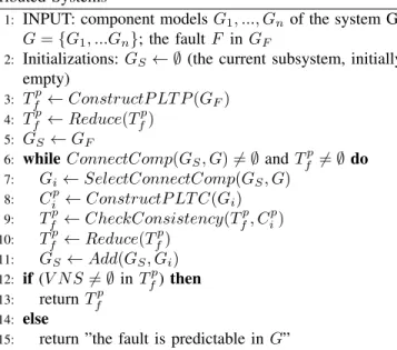
Algorithm 1 Polynomial Predictability Algorithm for
Dis-tributed Systems
1: INPUT: component models G1, ..., Gnof the system G:
G ={G1, ...Gn}; the fault F in GF
2: Initializations: GS← ∅ (the current subsystem, initially
empty)
3: Tfp← ConstructP LT P (GF)
4: Tfp← Reduce(Tfp)
5: GS ← GF
6: while ConnectComp(GS, G)̸= ∅ and Tfp̸= ∅ do
7: Gi← SelectConnectComp(GS, G) 8: Cip← ConstructP LT C(Gi) 9: Tfp← CheckConsistency(Tfp, Cip) 10: Tfp← Reduce(Tfp) 11: GS ← Add(GS, Gi) 12: if (V N S̸= ∅ in Tfp) then 13: return Tfp 14: else
15: return ”the fault is predictable in G”
Now we describe our distributed algorithm based on Theorem 10, which is optimized in the sense that we reduce the search space by distributing the analysis on the PLTP and PLTCs. As shown in the pseudo-code, algorithm 1 performs as follows. Given the input as the set of component models,
the fault F with the component GF, we first construct the
PLTP of GF and then reduce it to only retain all paths
containing critical normal states since any VNS is developed from a critical normal state in the original PLTP (line 3-4). Current subsystem GSis then assigned by GF (line 5). When
the consistent (reduced) PLTP of GS is not empty and there
exists at least one component connected to GS(line 6), which
means that the consistency of current PLTP should be further checked in an extended subsystem, the algorithm repeatedly performs the following steps:
1) Select one component connected to GS and construct
its PLTC. (line 7-8 )
2) The consistency of current PLTP is further checked by synchronizing with this PLTC based on their common left and right communication events with the constraint described in the precedent section. (line 9)
3) The newly obtained PLTP is reduced to keep only paths containing critical normal states. Then the extended subsystem is updated by adding this selected compo-nent. (line 10-11)
Note that each time we reduce the PLTP, we keep the same set of events. A (reduced) PLTP has the same set of events as the union of that of its renamed left and right instances of the corresponding diagnoser. In the same way, a PLTC has the same set of events as the union of that of its renamed left and right instances of the corresponding component. Only in this way, we can guarantee the correct synchronization of a reduced PLTP with a PLTC. Three cases can stop this algorithm:
• There is no connected component and there is at least
one VNS (line 12). From Theorem 10, the fault is not predictable. Thus, the algorithm returns the final PLTP providing useful information about VNSs (line 13).
• There is no connected component and the PLTP is not
empty but all the critical normal states retained are not VNSs, i.e., they have no reachable uncertain cycles and all components are directly or indirectly connected with each other. In this case, the algorithm returns the predictability information (line 14-15).
• The PLTP is empty, which implies that there is no VNS,
the predictability information is returned (line 14-15).
Theorem 11: Algorithm 1 has polynomial complexity
with the number of system states and exponential complexity with the number of faults.
Proof: From their construction, for a component Gi, the
maximum number of states and transitions of the diagnoser are (|Qi| × 2|Σif|) and (|Qi|2× 22|Σif|× |Σi|), respectively.
The maximum number of states and transitions of its PLTP (PLTC) are (|Qi|2×22|Σif|) and (|Qi|4×24|Σif|×|Σi|),
re-spectively. In the worst case, the global consistency checking consists in synchronizing PLTP (PLTCs) of all components. Thus, we can conclude that Algorithm 1 has polynomial complexity with the number of states and exponential com-plexity with the number of faults.
Note that the exponential complexity with the number of faults is for the case where we handle all faults simultane-ously. To reduce the complexity, our algorithm is illustrated by dealing with one fault each time.
V. CONCLUSION
In this paper, we propose a new polynomial approach for predictability analysis in a centralized way and then extend it to a distributed framework. First, we build the
PLTP for the faulty component GF to obtain the original
predictability information. Then we propose PLTCs for nor-mal components, which is synchronized with the PLTP re-specting a special constraint to check the global consistency. In reality, our distributed approach can greatly reduce the search space since each time we check consistency in an extended subsystem, we often keep a small subpart of current PLTP. Note that in our distributed case, the observations are globally available. Thus, predictability requires global occurrence order of observable events, for which we have to get some centralized information. This is also the case for most of distributed diagnosability algorithms developed in latest decades.
One close work to ours is the polynomial algorithm proposed in [5], where the authors directly use twin plant to analyze predictability in a centralized way. They check a pair of trajectories violating predictability that could lie in two different paths of twin plant, which is not suitable for distributed case. While we adapt twin plant to pre twin plant, where any pair of trajectories violating predictability can be caught by a path in pre twin plant. In this way, we can check their global consistency in a distributed way, i.e., whether the paths representing pairs of local trajectories violating predictability can survive after global consistency checking and contain VNSs.
One perspective of this work is that when the fault is not predictable, with the information returned by our algorithm, we can study whether it is possible to add sensors, i.e., make some unobservable events observable, to make the fault predictable. If the answer is positive, we can further investigate which unobservable events becoming observable can upgrade the predictability level. Another perspective is the probabilistic analysis of predictability for probabilistic discrete event systems. Inspired by the work [7] about prob-abilistic diagnosability, the objective would be to quantify by a probability or even more qualitatively the possibility of a fault occurrence in the future from present observations, which is a major issue for industrials.
REFERENCES
[1] S. Bavishi and E. K. P. Chong, “Automated fault diagnosis using a discrete event systems framework,” in Proceedings of the 9th IEEE
International Symposium on Intelligent Control, 1994, pp. 213–218.
[2] C. G. Cassandras and S. Lafortune, Introduction to Discrete Event
Systems. New York: Springer-Verlag, 2008.
[3] A. Cimatti, C. Pecheur, and R. Cavada, “Formal verification of diagnosability via symbolic model checking,” in Proceedings of the
20th International Joint Conference on Artificial Intelligence. San Francisco, CA, USA: Morgan Kaufmann, 2003, pp. 363–369. [4] S. Genc and S. Lafortune, “Predictability in discrete-event systems
under partial observation,” in Proceedings of the 6th IFAC Symposium
on Fault Detection, Supervision and Safety of Technical Processes,
Beijing, September 2006.
[5] ——, “Predictability of event occurrences in partially-observed discrete-event systems,” Automatica, vol. 45, no. 2, pp. 301–311, February 2009.
[6] S. Jiang, Z. Huang, V. Chandra, and R. Kumar, “A polynomial time algorithm for diagnosability of discrete event systems,” IEEE
Transactions on Automatic Control, vol. 46, no. 8, pp. 1318–1321,
2001.
[7] F. Nouioua and P. Dague, “A probabilistic analysis of diagnosability in discrete event systems,” in Proceedings of the 18th European
Conference on Artificial Intelligent, July 2008, pp. 224–228.
[8] Y. Pencol´e, “Diagnosability analysis of distributed discrete event systems,” in Proceedings of the 16th European Conference on Articifial
Intelligent, August 2004, pp. 43–47.
[9] M. Sampath, R. Sengupta, S. Lafortune, K. Sinnamohideen, and D. Teneketzis, “Diagnosability of discrete event system,” IEEE
Trans-actions on Automatic Control, vol. 40, no. 9, pp. 1555–1575, 1995.
[10] A. Schumann and J. Huang, “A scalable jointree algorithm for diag-nosability,” in Proceedings of the 23rd American National Conference
on Artificial Intelligence. AAAI Press, July 2008, pp. 535–540. [11] K. Sinnamohideen, “Discrete-event based diagnostic supervisory
con-trol system,” in Proceedings of the AIChE Annual Meeting, Los Angeles, CA, 1991.
[12] N. Viswanadham and T. L. Johnson, “Fault detection and diagnosis of automated manufacturing systems,” in Proceedings of the 27th
Conference on Decision and Control, Austin, TX, 1988, pp. 2301–