Cosmological constraints from the virial mass function of nearby galaxy groups and clusters

Cosmological Constraints from the Virial Mass

Function of Nearby Galaxy Groups and Clusters

by

James Colin Hill

Submitted to the Department of Physics

in partial fulfillment of the requirements for the degree of

Bachelor of Science

at the

MASSACHUSETTS INSTITUTE OF TECHNOLOGY

June 2008

@ James Colin Hill, MMVIII. All rights reserved.

The author hereby grants to MIT permission to reproduce and

distribute publicly paper and electronic copies of this thesis document

in whole or in part.

Author.

Department of Physics

May 16, 2008

Certified by.

(I

_{Professor Claude R. Canizares}

Department of Physics

Thesis Supervisor

Certified by..

Dr. Kenneth J. Rines

Harvard-Smithsonian Center for Astrophysics

Thesis Supervisor

Accepted by ...

Professor David E. Pritchard

Senior Thesis Coordinator, Department of Physics

MASSACHUSETTS INSTiTUTE

OF TECHNOLOGY

JUN 132008

Cosmological Constraints from the Virial Mass Function of

Nearby Galaxy Groups and Clusters

by

James Colin Hill

Submitted to the Department of Physics on May 16, 2008, in partial fulfillment of the

requirements for the degree of Bachelor of Science

Abstract

In this thesis, I present a new determination of the cluster mass function in a volume 107 h -3 Mpc3 _{using the ROSAT-2MASS-FAST Group Survey (R2FGS). R2FGS is} an X-ray-selected sample of systems from the ROSAT All-Sky Survey in the region 6 > 0' and 0.01 < z < 0.06, with target galaxies for each system compiled from the Two Micron All Sky Survey (2MASS). The sample is designed to focus on low-mass groups and clusters, so as to break a degeneracy between the cosmological parameters m, and os. In addition, R2FGS covers a very large area of sky (, 4.13 ster.), which is necessary given the low redshift limit of the survey. I acquire optical redshifts for the target galaxies in R2FGS from the literature and from new data collected with the FAST spectrograph on Mt. Hopkins. After removing foreground and background galaxies (interlopers) using a dynamical maximum-velocity criterion, I estimate the group and cluster masses using the full virial theorem, and subsequently verify the results using the projected mass estimator. I briefly investigate the up - Lx

and M - Lx scaling relations, as well as the halo occupation function. Due to

interloper issues with some of the systems, I apply a luminosity-dependent correction to the virial masses, and subsequently use these masses to compute the virial mass function of the sample. By comparing this mass function to predictions from various cosmological models, I constrain the parameters •,m and 8s. I find Qm = 0.26 +0.07

and U8 = 1.02 +3; the R2FGS value for Qm agrees very well with the recent

Five-Year WMAP (WMAP5) result, although the R2FGS value for as is somewhat larger than that found by WMAP5. Future work will include an expansion of the survey to 6> -200 and z < 0.04, which will greatly increase its degeneracy-breaking power. Thesis Supervisor: Claude R. Canizares

Title: Professor of Physics

Thesis Supervisor: Dr. Kenneth J. Rines

Acknowledgments

First, I would like to thank Ken Rines for his extensive help and advice over the past year, as well as for giving me the opportunity to work on such an interesting project. I would also like to thank Prof. Claude Canizares for his helpful advice and support as my co-supervisor. In addition, I am grateful to Prof. Max Tegmark and Molly Swanson for their guidance and collaboration with me on my first research project in cosmology, and to Prof. Scott Hughes for introducing me to astrophysics research three years ago. Without the support of so many great advisors, I would never have successfully completed such a breadth of research during my undergraduate years.

Second, I am eternally grateful to my friends, without whom I surely would not have survived MIT; I have learned more about physics, math, and tomfoolery from them than any class could ever teach. Most important, I owe great thanks to my family, particularly my parents, who have always encouraged and supported me in everything I do, especially in the form of banana bread and coffee. I could not have made it this far without them.

Contents

1 Introduction 13

1.1 The (Qm, 8) Degeneracy . ... .. 14

1.2 The Cluster Mass Function . ... . 15

1.2.1 Mass Estimation Techniques . ... . 15

1.2.2 Recent X-ray Studies . ... .. 16

1.2.3 The CIRS Mass Function . ... . 17

1.2.4 The R2FGS Mass Function . ... . 18

2 The R2FGS Sample 21 2.1 X-ray Cluster Surveys ... ... 21

2.2 Group and Cluster Selection . ... . 22

3 The R2FGS Observations 25 3.1 Target Galaxy Selection . ... . 25

3.2 FAST Data ... ... ... 26

4 Estimating Cluster Masses 27 4.1 Interloper Removal .. ... . 27

4.2 Virial Masses .. ... . 30

4.3 Projected Masses .. ... .. 31

4.4 The Reduced R2FGS Sample . ... 32

5 Cluster Scaling Relations 35 5.1 The Velocity Dispersion-Luminosity Relation . . . . . . . .... . 35

5.2 The Mass-Luminosity Relation . . . .. 36 5.3 The Velocity Dispersion-Mass Relation . . . . 38 5.4 The Halo Occupation Function ... . . . . . . . . . ..... 40

6 The R2FGS Mass Function 45

6.1 Uniform Correction ... ... 47

6.2 Luminosity-Dependent Correction . . . . 47 6.3 Comparison to Previous Mass Functions . . . . 49

7 Cosmological Constraints 55

8 Conclusions 59

A Redshift-Radius Plots 61

List of Figures

6-2 R2FGS mass function: uniform correction . . . . . 48

6-3 R2FGS mass function: luminosity-dependent correction . . . . . 50

7-1 Constraints on Qm and 8s . . . 58

A-1 Acz versus Rp for the first ten R2FGS systems (ordered by increasing cluster redshift).. . . . 62

A-2 Acz versus Rp for the next ten R2FGS systems . . . . . 63

A-3 Acz versus Rp for the next ten R2FGS systems . . . . . 64

A-4 Acz versus Rp for the next eight R2FGS systems . . . . . 65

A-5 Acz versus Rp for the next eight R2FGS systems . . . . . 66

A-6 Acz versus Rp for the next eight R2FGS systems . . . . . 67

List of Tables

B.1 R2FGS Groups and Clusters . ... . 69 B.2 R2FGS Systems: M20 0, MpM, MLx, r200, 2 00 . . . . . .

Chapter 1

Introduction

The observed abundance of massive systems as a function of mass, that is, the mass

function, is a basic prediction of any viable cosmological model. The hierarchical

theory of cosmic structure formation asserts that groups and clusters of galaxies arise from rare high peaks of the initial density fluctuation field, and currently represent the most massive virialized systems in the universe. These systems are a powerful and fairly clean tool for cosmology because their growth is primarily governed by linear gravitational processes, as first described analytically by Press and Schechter [1];

their theory implies that the abundances of groups and clusters depend strongly on the amplitude of the density fluctuations on the cluster mass scale. In particular, these abundances are highly sensitive to Qm, the matter density of the universe, and os, which is both the rms amplitude of the density fluctuations on an 8 h- 1

Mpc scale and the normalization of the linear power spectrum [2, 3]. Moreover, the evolution of the mass function is a measure of the growth of structure, and can therefore be used to constrain the (possibly redshift-dependent) properties of dark energy [4, 5, 6, 7, 8, 9, 10]. In order to obtain robust constraints on this evolution, though, an accurate measurement of the mass function in the nearby universe is needed.

1.1

The

(Qm,

Degeneracy

Although the cluster mass function is a sensitive probe of Qm and us, there is a large degeneracy in this parameter space for high-mass systems: for example, a small value of as (for a given power spectrum) implies that massive clusters are very rare peaks in8

the initial density field, and thus predicts a low abundance of such clusters; however, a similar effect would follow from a small value of Qm, as a smaller amount of matter in the universe would lead to a smaller abundance of massive clusters. Similarly, a large value of as implies that large fluctuations in the density field (which then form8

massive clusters) are more common; again, though, this effect could also occur due to a larger value of Qm, as a larger amount of matter in the universe would yield a larger abundance of massive clusters. However, two models that predict the same number of high-mass clusters predict different abundances of low-mass clusters: the model with the smaller value of as predicts fewer low-mass clusters than the model₈ with the larger value of us. Therefore, it is important to accurately determine the cluster mass function at group-scale masses, where the degeneracy between Qm and

8

as can be broken by probing not just the amplitude of the mass function, but also its shape.

Recent estimates of as from the local cluster mass function include values in8

the range as 8 0.6 - 0.8 for Qm = 0.3 [11, 12, 13, 14, 15, 16, 17, 18, 9, 19, 20]. Somewhat larger estimates of as 8 0.8- 1.0 have also been obtained recently through

the measurement of cosmic shear [21, 22], which is the distortion of light emitted by distant background galaxies while traveling through the universe, producing a small effect on the distribution of galaxy ellipticities. The recently-released Five-Year WMAP results (WMAP5) found a8 = 0.796+0.036 [23]; recent modeling work has also

converged on values in the range as8 0.7 - 0.9 [24].

However, until the release of WMAP5, there was significant tension between the WMAP3+SDSS results [25] and CDM simulations [24]: the WMAP3+SDSS cosmol-ogy required significant velocity segregation in clusters and excess specific energy in the intracluster medium (ICM) in order to explain discrepancies in the value of the

parameter Ss = 9s(Qm/0.3)0

.3 5_{. These requirements conflicted strongly with}

expecta-tions from numerical simulaexpecta-tions. However, the revised constraints from WMAP5 [23]

are sufficient to require only modest velocity segregation and small specific energy in the ICM, while those from WMAP5+SN+BAO [26] actually make both of these requirements unnecessary [27]. In particular, the revisions between WMAP3 and WMAP5 bring their results into much better agreement with the recent cluster mass

function of Rines et al [28].

In short, observational estimates of the cluster mass function provide important cosmological constraints. In this thesis, I attempt to improve these constraints by sampling a larger area of sky and probing smaller cluster masses than previous studies.

1.2

The Cluster Mass Function

1.2.1

Mass Estimation Techniques

The largest obstacle to accurately estimating the cluster mass function is comput-ing sufficiently accurate mass estimates. There are three well-known techniques for obtaining such estimates:

1. Applying the virial theorem to observations of the dynamics of cluster galax-ies [29, 30];

2. Observing the properties of the hot ICM, whose distribution and temperature depend strongly on the cluster's gravitational potential [31];

3. Measuring the gravitational lensing of background clusters by foreground ob-jects, which produces very accurate mass estimates in the centers of clus-ters (first suggested by Zwicky [30]).

Each of these techniques is subject to possibly large systematic uncertainties. Tech-nique (1) may be inaccurate due to the presence of substructure, as well as velocity bias between cluster galaxies and dark matter particles, although the exact magnitude and direction of this bias is still a matter of debate [32, 24]. Method (2) is subject

to uncertainties resulting from the complex physical properties of the ICM and its interaction with active galactic nuclei (AGN), as demonstrated in observations from

Chandra and XMM-Newton [33], although this is only a significant problem in the

cores of clusters. Finally, errors may arise in method (3), especially at large radii, due to lensing by other objects (e.g., filaments) along the line-of-sight to the clus-ter [34, 35]; however, such errors may be overcome by combining observations of both strong and weak lensing [36, 37]. As a result of these potential uncertainties, some groups have instead determined cluster properties in an inverse fashion by match-ing the mass function predicted by a cosmological model to the measured luminosity function or richness function [38, 39].

1.2.2

Recent X-ray Studies

The cluster mass function has been studied extensively in recent years, primarily via X-ray data [12, 40, 9] or optical richness data, i.e., the number of galaxies found in a cluster via optical observations, subject to some magnitude criterion [18]. Mea-surements of the mass function using X-ray data are subject to several sources of uncertainty. First, the most significant uncertainty is due to the normalization of scaling relations, namely, that of M - Tx or M - Lx [41], for which a range of values

has been determined in hydrodynamical simulations [42, 15, 17]. Additionally, these scaling relations may be subject to Malmquist bias [39]. Some investigators avoid such scaling relations altogether by estimating the mass of the ICM and measuring the baryonic mass function [9, 43], although this technique requires additional as-sumptions regarding the relative contribution of stars and gas to the total baryon mass, the ratio of the baryon fraction in clusters to the global value of the baryon fraction, and the mass dependence of this ratio.

Secondly, all of these X-ray studies are subject to a potentially large systematic error (- 20 - 30%) resulting from a difference between the temperature Tspec

mea-sured by X-ray satellites and the emission-weighted temperature Tew computed in the aforementioned simulations [44]. This effect arises due to an ICM with a variety of temperatures, leading to an excess contribution of line emission from cooler gas,

which causes Tspec to underestimate Tew. However, this effect should not pose a prob-lem if observations of the cores of clusters are omitted. Vikhlinin et al. [45] found a similar systematic effect, namely, a higher normalization of the mass-temperature relation using Chandra observations of the temperature profiles of relaxed clusters, which would lead to an increase in both the estimated cluster masses as well as the

inferred constraints on Qm and u8s.

Finally, some investigators have combined X-ray data with weak lensing measure-ments to compute the mass function [14, 20], and have obtained results generally consistent with those of other X-ray techniques.

1.2.3

The CIRS Mass Function

The most recent observation-based cluster virial mass function is that computed from the Cluster Infall Regions in SDSS (CIRS) sample [28]. Virial mass estimates have improved dramatically in recent years as a result of the size and uniformity of large-scale redshift surveys, such as the Sloan Digital Sky Survey [46] (SDSS). Furthermore, virial mass estimates provide several advantages over X-ray studies: they are sensitive to larger scales (r2o0o rather than r500oo); they can be compared with theoretical mass

functions with much less extrapolation [47]; they are less sensitive to the complicated physics in the centers of clusters; and virial masses can be estimated for poor clus-ters and rich groups, while X-ray mass estimates for these systems are complicated

by nongravitational physics, such as energy from AGN [48]. Importantly, the mass estimates for these low-mass systems allow one to eliminate any uncertainty resulting from the possible scale dependence of the estimate of as; in other words, one directly8 constrains fluctuations on the scale 8 h-1 Mpc, as opposed to the -, 14 h-1 Mpc

scales probed by - 1015 h- 1 M® clusters [11]. Recently, Eke et al. [19] estimated the group mass function from an optically-selected group catalog in the 2dFGRS [49] using a simplified version of the virial theorem. However, estimates of the group mass function based on measurements of virial masses can be hindered by systematic uncertainties in the group selection function, mass estimation techniques, and cosmic variance [50, 51, 52].

Rines et al. [28] improve on this measurement by overcoming many of these dif-ficulties. First, they utilize X-ray selection rather than optical selection of clusters, which both reduces the influence of projection effects and allows the selection func-tion to be computed directly. Second, they compute virial masses using the full virial theorem, including corrections for the surface pressure term [53, 54, 55]. Third, the CIRS survey [56] includes much better sampling of individual systems than the 2dF-GRS catalog. Finally, they remove interlopers in a much more conservative manner, thus greatly reducing scatter in the mass estimates. With the CIRS mass function

alone, they find 8 = 0.84 + 0.03 when holding •m = 0.3 fixed.

1.2.4

The R2FGS Mass Function

This thesis is a complementary study to that of Rines et al [28]. In particular, it is difficult to measure the abundance of X-ray groups and clusters of - 1014 MD

from SDSS data, since available X-ray surveys detect these systems only in the very nearby universe, and SDSS does not cover the whole sky (although it does cover a large volume of space). Hence, R2FGS is designed to cover a much larger area of sky to a shallower depth; in fact, the area of the R2FGS region is nearly twice the area of the SDSS DR6 spectroscopic footprint. To construct the R2FGS dataset, I utilize an X-ray selected sample from the ROSAT All-Sky Survey (RASS) group and cluster catalogs [57]. I then select targets in these systems from 2MASS [58]. I combine these measurements with optical redshift data found in the literature, as well as new data collected with the FAST spectrograph on Mt. Hopkins in Amado, AZ.

After carefully removing interlopers, I estimate the virial masses of these X-ray-selected systems and compute the mass function. Note that this study avoids sig-nificant problems with Malmquist bias (despite using an X-ray selected sample) by using virial mass estimates that do not depend on X-ray data, as well as by using the Vmax weighting technique in my calculation of the mass function. I also use the virial mass data to probe the scaling relations between X-ray luminosity and virial masses over a wide mass range. This result is important for future measurements of the evolution of cluster abundances, which will be used to constrain the properties of

dark energy. In addition, I use the virial mass data to investigate the halo occupation function, which is an important link between numerical simulations and observables, especially in studies of galaxy formation [59]. Finally, by measuring the slope of the mass function at low mass, I break the aforementioned degeneracy between Qm and os, and obtain constraints on these cosmological parameters.

The remainder of this thesis is organized as follows. In §2, I describe the data and the cluster sample. In §3, I discuss observations taken for this project. I estimate the group and cluster virial masses in §4. I examine the up - Lx, M - Lx, and

N - M scaling relations in §5. In §6, I compute the mass function. I then constrain

the aforementioned cosmological parameters in §7. Finally, I discuss the results and conclude in §8. I assume H0 = 70h70 km s- 1, and a flat ACDM cosmology (QA =

1 - Qm) throughout. Where not stated otherwise, I assume Qm = 0.3 and h70 = 1.0 for initial calculations when necessary.

Chapter 2

The R2FGS Sample

2.1

X-ray Cluster Surveys

This study is primarily focused on low-mass systems. As these systems are rather faint in X-ray emission, RASS only finds them in the very nearby universe (z < 0.06). Although RASS is a shallow survey, it covers essentially the entire sky and is the most complete X-ray survey for nearby groups and clusters. Conveniently, 2MASS provides photometry over the entire sky to a depth corresponding to M* + 1 for these systems, where M* is the magnitude of the characteristic knee in the Schechter function describing each system's luminosity [60]. CIRS showed that this depth is sufficient to obtain large samples of cluster galaxies needed for accurate dynamical mass estimates [28].

Moreover, R2FGS is unique in that it covers a much larger area of sky than previous mass function surveys (or even the SDSS). In particular, the area of the R2FGS footprint is r 4.13 ster., nearly 3 times larger than the CIRS mass function area of - 1.46 ster. For comparison, the area of the SDSS DR6 spectroscopic footprint is - 2.26 ster. Thus, although R2FGS is not a particularly deep survey, it still includes

a significant volume of space due to the large size of the survey region.

The exact criteria for group and cluster selection are described below. I search several published cluster catalogs derived from RASS, including: the X-ray Brightest Abell Cluster Survey (XBACS, [61]); the Bright Cluster Survey and its extension

(BCS/eBCS, [62, 63]); the NOrthern ROSAT All-Sky galaxy cluster survey (NORAS, [64]); and the ROSAT-ESO Flux-Limited X-ray galaxy cluster survey (REFLEX, [65]). For detailed descriptions of the construction of the catalogs, please consult the original catalog papers (see Rines and Diaferio [56] for a summary).

None of these catalogs is complete; the worst, NORAS, is - 50% complete, while the best, REFLEX, is - 90% complete. Regardless, I obtain a fairly com-plete composite catalog after combining them (more comcom-plete than any individ-ual catalog). In particular, as mentioned above, the composite catalog covers es-sentially the entire northern sky at high Galactic latitude

(Ibl

Galactic absorption). Since the catalogs are nominally complete to a flux limit of

fx 3 x 10- 12 erg cm- 2 s- 1, my imposed flux limit ensures that the sample is essen-tially fully complete. For the purposes of this study, I disregard any modest possible incompleteness, as these clusters are an unbiased sample selected purely based on X-ray flux. I confirm this claim with a V/Vmax test [66]: I find (V/Vmax) = 0.492 + 0.038 compared to an expected value of 0.5 for a complete, uniform sample.

When the composite catalog contains multiple X-ray fluxes for a given cluster, I choose the most recently published value. Hence, the order of preferences is: RE-FLEX, NORAS, BCS/eBCS, XBACS. Note that the various surveys determine fluxes in somewhat different ways: REFLEX and NORAS measure fluxes with Growth Curve Analysis (GCA), while BCS/eBCS utilizes Voronoi Tessellation and Perco-lation (VTP). Nevertheless, the measured fluxes are in fairly good agreement; see Figure 21 of B6hringer et al. [64] for a direct comparison of NORAS and BCS/eBCS. Note that since I use the most recently published flux value, my first preference is GCA, while my second is VTP.

2.2

Group and Cluster Selection

The overall observational goal for this study is to obtain complete spectroscopic sam-ples to roughly the 2MASS magnitude limit [58] for all groups and clusters in the

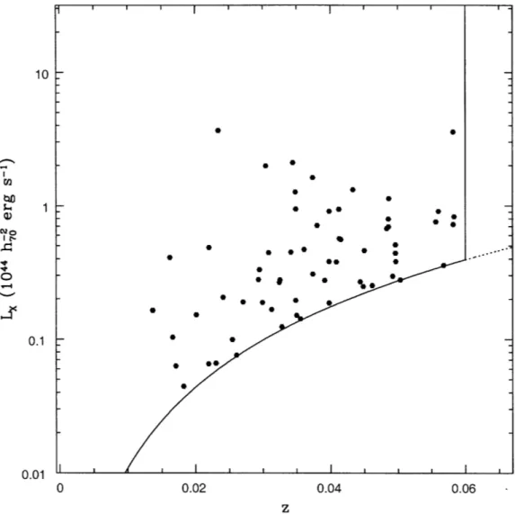
ROSAT catalogs, restricted to the region 6 > 00 and 0.01 < z < 0.06, in addition to the flux limit described above. Note that the aforementioned differences in the flux determination techniques for the various surveys may slightly alter the exact flux limit. After imposing these restrictions, the sample consists of 62 groups and clusters, which I will hereafter refer to as the R2FGS systems. Figure 2-1 shows the redshift versus X-ray luminosity of each R2FGS system, as well as the sample X-ray luminos-ity and redshift limits. A complete list of the R2FGS systems and their properties is given in Table 1 of Appendix B.

'IO t.4 CQ It4. J-4 0.1 .V I 0 0.02 0.04 0.06

Figure 2-1: Redshift versus X-ray luminosity (0.5 - 2.0 keV) for X-ray clusters from XBACS, BCS/eBCS, NORAS, and REFLEX contained in the R2FGS region. The X-ray cluster catalogs are nominally complete to fx 3 x 10- _{12 erg cm}-_{2 S-1; thus,}

the imposed R2FGS limit of fx > 5 x 10-12 erg cm -2 _s-1 _{(denoted by the solid curved}

line) ensures that the R2FGS sample is essentially fully complete. The solid vertical line shows the R2FGS redshift limit.

Chapter 3

The R2FGS Observations

3.1

Target Galaxy Selection

For a given cluster, I select as targets all galaxies in 2MASS within a projected dis-tance Rp = 2.14 Mpc/h 70 of the cluster's X-ray center, such that either the galaxy's

Kron magnitude K, < 13.0 or its absolute magnitude MK, < -22.2 + 5 log h70

(- Mk + 1), where I assume the target galaxy is at the distance of the cluster. I

supplement the 2MASS redshift catalogs with literature data from the NASA/IPAC Extragalactic Database (NED) and from the SDSS for galaxies fainter than the mag-nitude limits stated above.

Approximately half of the targets in the sample have already been surveyed with the FAST spectrograph for the 2MASS Abell Cluster Survey [67], and about half of the remaining systems are included in SDSS Data Release 6 (DR6) [68]. The process of obtaining spectra with the FAST spectrograph for galaxies in the • 25 remaining systems is nearly complete; A2665, A2626, and A2271 are the only remaining systems with significant incompleteness. Overall, I have targeted 1048 galaxies in groups and clusters across the northern sky, 964 of which have been observed through January 2008. Combined with existing redshift data, the entire survey includes - 14800 galaxies, for an average of - 240 galaxies per field and - 120 members per system

3.2

FAST Data

The new redshifts were obtained with the FAST spectrograph [69] on the 1.5-m Till-inghast telescope at the Fred Lawrence Whipple Observatory (FLWO) in Amado, AZ. FAST is a high-throughput, long-slit spectrograph with a thinned, backside-illuminated, antireflection-coated CCD detector. The length of the slit is 180"; the R2FGS observations used a slit width of 3" and a 300 lines mm - grating. This setup provides spectral resolution of 6 - 8A and spans the wavelength range 3600 - 7200A. Redshifts are computed by cross-correlation with spectral templates of emission-dominated and absorption-emission-dominated galaxy spectra created from FAST observa-tions [70]. The uncertainty in the redshifts is usually < 30 km s 1.

One significant difference between the FAST spectra collected for this project and those collected for other redshift surveys [49, 46] is that the completeness of the R2FGS sample is not hindered by fiber placement constraints. Another difference is that the long-slit FAST spectra sample light from larger fractions of galaxy areas than do fiber spectra. Hence, the effects of aperture bias on spectral classification are significantly lessened [71, 72].

Chapter 4

Estimating Cluster Masses

4.1

Interloper Removal

The removal of interlopers is a challenging problem in any galaxy cluster study. Re-cently, Wojtak et al. used cosmological N-body simulations to perform a detailed analysis of many widely-used interloper removal schemes [73]. Of all the direct meth-ods, they recommend a dynamical maximum velocity criterion first proposed by Den Hartog and Katgert [74]. This method removes the largest fraction of interlopers (73%) and avoids many of the difficulties of indirect methods, such as the need for large kinematic samples that can only be obtained by stacking data from many ob-jects.

Based on these results, I utilize this dynamical maximum velocity criterion in this thesis. In this method, I select as an interloper any particle at a given projected radius R whose velocity exceeds a maximum attainable velocity for halo particles at this radius. For the maximum velocity profiles, I consider two characteristic velocities: the circular velocity Vcjr and the infall velocity Vinf, given respectively by

vir = v/GM(r)/r (4.1)

Vinf

vfVcir.

(4.2)

theorem is violated; it can be thought of as an escape velocity from the mass interior to the radius r [73].

The following formula then gives the maximum velocity profile:

Vmax = maxR {vinf cosO, Vcir sin O}, (4.3)

where 0 is the angle between the position vector of the object with respect to the cluster center and the line of sight. This formula assumes a particular kinematic model that allows objects to fall onto the cluster center with velocity Vinf or to move tangentially with circular velocity vir. This is a fairly restrictive maximum velocity criterion, which gives accurate limits at large R - rvir [73].

The final component needed for the maximum velocity profiles is the mass profile. In accordance with the rest of this study, I utilize the mass estimator MVT derived from the virial theorem [75]:

MvT(r = Rmax)- 37N Ei (v )2 (4.4)

2G -i.j1/ Rij

where N is the number of galaxies enclosed on the sky by a circle with radius Rmax,

vi is the line-of-sight velocity of the ith galaxy, and Ri,j is the projected distance between the ith and jth galaxies. Note that this formula is valid for spherical systems

with arbitrary anisotropy. I then approximate the mass profile as M(r) _ MVT(Ri <

r < Ri+I), where Ri is the sequence of projected radii of galaxies in increasing order. However, the virial theorem applies to an entire system; thus, since I am applying it to a subset of the cluster members, a surface pressure term is required: 2T + U = 3PV,

instead of the usual 2T + U = 0 [55]. However, as I am concerned here with interloper removal and not accurate mass estimation, I neglect the surface term in this analysis, although it is included in the final mass estimates (see §4.2).

In order to determine cluster membership, I initially include all galaxies within S2.5 h- 1 Mpc of a given cluster X-ray center (larger radii are used for some clusters that clearly have a large virial radius, such as Coma and A2147). I then apply the Vmax criterion described in the preceding paragraphs, so as to discard any galaxies

with vi > Vmax. Figures A-1-A-7 in Appendix A display the infall patterns for all

62 groups and clusters in the R2FGS sample, starting with NGC1550 (z = 0.0131), the nearest cluster in the sample, and increasing in redshift up to A2457 (z = 0.0594), the most distant cluster in the sample. The plots show both interlopers and member galaxies, as well as the maximum velocity profiles calculated using Eq. (4.3). Most of the systems have a sufficient amount of data to accurately estimate their virial mass, although FAST data is still being collected for a few (e.g., A2271). Interest-ingly, several of the systems in the R2FGS sample have very few existing redshifts in the literature, despite their proximity. For instance, 2A0335, which has been ob-served extensively with Chandra [76], had only two published redshifts before this new survey.

Lastly, note that there appear to be interlopers remaining in some systems (e.g., UGC04052, NGC4325, A1142, and A2626) after the removal procedure described above. This is partly an unfortunate consequence of the fact that the fraction of removed interlopers is limited in principle to values less than 75% using the Vmax technique, because - 1/4 of the unbound particles within the observation cylinder are within the envelope of bound velocities and hence inaccessible to direct removal techniques [73]. Further analysis of particularly outlying objects, such as those in A2626, may be needed before a truly robust virial mass estimate for such systems can be obtained. Perhaps the most difficult system to analyze in the entire sample is A2147, a member of the Hercules supercluster (with A2151 and A2152). Due to the extreme proximity of the two other clusters, it is very difficult to accurately determine cluster membership for A2147; rather sophisticated interloper removal techniques are required, such as the KMM mixture-modeling algorithm [77]. In general, though, the Vmax technique successfully removes most of the evident interlopers from the R2FGS systems.

4.2

Virial Masses

After removing interlopers from each system, I use Eq. (4.4) to compute the virial masses. To start with, it is necessary to define a radius of virialization within which the member galaxies are relaxed. I use r200, where rA refers to the radius at which the mean enclosed density is Ape, where Pc is the critical density:

3H

2

PC = (9.21 x 10-27 kg m-3)h 20 . (4.5)

8-7rG 70×

If the system does not lie completely within r20 0, the surface pressure term 3PV

in the virial theorem must be included, as described in the previous section. The virial mass is then an overestimate of M200, so that a correction C must be applied.

Assuming that mass follows the galaxy distribution, the correction is given by

47rr3 _p(r200oo)

[

2 2 ) (4.6)

f

200 47rr2_{pdr [o(< r}

2o00) '

where r,(r 20oo) is the radial velocity dispersion at r200 ooand u(< r200oo) is the inte-grated velocity dispersion within r20 0 [78]. Considering the limiting cases of circular,

isotropic, and radial orbits, the maximum values of the term involving the velocity dispersion are 0, 1/3, and 1, respectively.

After obtaining an initial estimate of r20 0 using the mass profiles calculated from

the interloper-cleaned systems, I apply a correction factor of 8% to account for the aforementioned surface term. This factor is calculated from Eq. (4.6) assum-ing isotropic orbits of galaxies and an NFW mass profile [79] with a concentration parameter c2 0 0 = r200/rs = 5, where r, is a scale radius in the NFW profile. Note

that the assumption of isotropic orbits is supported by many observations [32], as is the value c200 = 5 [80]. After this correction, the enclosed density within r20 0 is 17 8pc; thus, I reduce the corresponding estimate of M200 by 3.3%.

Lastly, I estimate the uncertainties on the virial masses by using the limiting fractional uncertainty 7r-V 2lnNN- 1_/2 _{[81]. Note that these uncertainties do not}

Appendix B lists the M200 and r200 estimates.

Unfortunately, I am not able to obtain mass estimates for four of the systems in the R2FGS sample using the techniques described above, because the density enclosed by any projected radius R never drops below 2 0 0Pc. I instead estimate the virial masses of these systems by letting M200 be the total mass enclosed by the projected radius of the most distant galaxy (from the cluster center) left after interloper removal. I then estimate r200 using the relation

(

3

M2

oo

7200

=

(4.7)

8007F _Pc

The groups and clusters for which I use this method are A2147, A0576, MKW3s, and A2256. The reasons behind the failures of these systems to converge to Pend < 2 0 0pc

appear to be mostly related to interlopers. The difficulties of analyzing A2147 were already discussed in the previous section, but its failure to converge demonstrates the seriousness of the aforementioned membership assignment problems. For A0576, it appears that interlopers within the bound velocity envelope are responsible. For MKW3s, the maximum velocity scheme evidently fails to remove several galaxies far outside the infall region, which are very likely interlopers. Essentially, the interlopers remaining in these three systems lead to a significant overestimate of the enclosed mass at a given radius, so that the enclosed mean density is never < 200pc (at least not within radii of < 3h-1 Mpc). A2256, on the other hand, simply seems to be an extremely massive cluster, and it is not particularly surprising that its enclosed density does not converge in this scheme.

4.3

Projected Masses

As a "sanity check" on my calculation of the virial masses, I confirm these results using the projected mass estimator MpM [81]:

MPM(r

=

R

)

(Vi

i,

(4.8)

where N is the number of galaxies lying within a distance R200 of the cluster center, vi is the line-of-sight velocity of the ith galaxy, and Ri is the projected radius of the ith galaxy with respect to the cluster center. The parameter a is intended to account for the difference between measuring velocities and radii relative to the center of mass of the system and measuring these quantities relative to the centroid of the tracers. Following Heisler et al., I set a = 1.5, which is appropriate for radial or isotropic orbits [81]. The parameter fPM is equal to 64/w for radial orbits and 32/7 for isotropic orbits [81]; I use the value 32/7, since I have no specific information regarding the distribution of orbit eccentricities. Finally, I approximate the fractional uncertainty

on MpM as 1.4/vN.

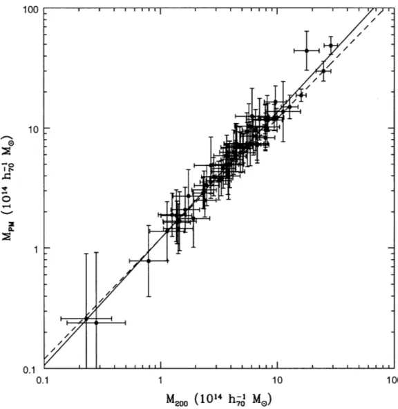
The projected mass estimator avoids some of the difficulties encountered by the virial mass estimator. For example, it is less sensitive to galaxies which are acciden-tally projected very close to each other. Thus, it provides a good method with which to confirm the virial mass results above. I calculate MPM for each system using all of the member galaxies within r200; the results are listed in Table 2. In addition, to investigate the correlation of these two mass estimators, I plot MPM versus M200 in Figure 4-1. In an idealized situation, I would expect the best-fit line to have a slope of 1 (the dashed line in the figure). Computing the bisector of the two weighted least-squares fits, I find a slope of 1.053

+

Finally, although the projected mass estimator is a useful tool for comparison, the virial mass estimator is still generally preferred for galaxy cluster studies, since it does not require any model-dependent parameters which must be specified by hand. Hence, I utilize only the M200 estimates throughout the rest of this thesis.

4.4

The Reduced R2FGS Sample

Although the Vmx,, _{scheme is fairly effective when applied to the R2FGS systems,} there are still many groups and clusters that appear to contain interlopers even after

100 10 0_IUU 1 0 U.I 0.1 1 10 100

M

oo

(1014

h-o

Me)

Figure 4-1: M200 versus MpM. The solid line displays the bisector of the weighted least-squares fits: logloMpM = (1.053 ± 0.017)logIoM 200oo + (0.078 ± 0.016). For

applying the removal algorithm. In some cases, this is due to a sparseness of data, but in most, it is due to the presence of galaxies which hinder the effectiveness of a generalized algorithm. One possible solution to this problem is to apply a different interloper removal technique for each system (e.g., the "shifting gapper" technique [82] or the M2oo/MPM ratio test technique [73]). However, this would come at the cost00

of generality in the analysis; it is a delicate procedure to combine data sets analyzed using very different techniques.

Nevertheless, in order to calculate a robust mass function and accurately constrain

Qm and Us, the masses utilized in the analysis must be very accurate. For many of the R2FGS systems, the redshift-radius plots given in Appendix A demonstrate that this is clearly not the case. Therefore, based on a visual inspection of the phase-space plots, I define a "reduced" R2FGS sample which consists only of those systems that appear to be accurately analyzed by the Vmax interloper removal technique (e.g., Coma or A2052). Since this is a difficult issue to define precisely, I err on the side of caution and attempt to leave in any system that does not have clear problems in its redshift-radius plot.

As a characteristic example of a problematic system, consider A2063. Upon visual inspection, this system appears to have a well-defined caustic profile; however, the Vmax criterion (denoted by the solid black curve) is significantly weakened by the presence of a handful of outlying objects at large projected radii. An interloper removal scheme based on deviations from the mean, such as the shifting gapper technique [82], would likely identify these particles as interlopers. As such, I do not include this system in the reduced R2FGS sample. Overall, after similarly analyzing all 62 groups and clusters, I include 45 in the reduced sample. The 17 clusters which do not pass the cut are marked with an asterisk (*) in Table 2 of Appendix B.

Finally, this cut introduces an incompleteness in the sample which must be taken into account when calculating the mass function. I consider two methods of account-ing for this incompleteness in §6.1 and §6.2; the second method relies upon usaccount-ing the reduced R2FGS sample to calibrate scaling relations between Lx and M200 and U200, which is the main focus of the following chapter.

Chapter 5

Cluster Scaling Relations

Scaling relations between simple cluster observables (e.g., temperature or luminos-ity) and cluster masses probe the nature of cluster assembly, as well as the detailed properties of cluster components. It is extremely important that these relations are well-established for clusters in the local universe, as future studies of distant clusters that aim to constrain dark energy will rely on these results.

5.1

The Velocity Dispersion-Luminosity Relation

I utilize the results of Danese et al. to calculate the mean redshift c2 and the projected velocity dispersion

up

n v2 2

2PZ _(5.1)

=

n - 1 (I

+ VP/c)2

where vp, = (Vp1 - Vp)/(1 + Vp/c) is the line-of-sight component of the velocity of the ith galaxy with respect to the cluster center of mass, Vp, = czi is the radial velocity of the ith galaxy uncorrected for the motion of the local observer, Vp = cf , and 6 is the uncertainty in the measured values of cz. For this study, I am particularly interested in the velocity dispersion at r200, denoted by UO200, which I calculate for

R2FGS groups and clusters are given in Table 2 of Appendix B.

Perhaps the simplest cluster observable is X-ray luminosity. The X-ray luminosi-ties for the systems in the R2FGS sample are in the ROSAT band (0.5 - 2.0 keV) and corrected for Galactic absorption. Figure 5-1 shows U200 versus Lx, using the

veloc-ity dispersions given in Table 2 of Appendix B. The solid dots in the figure represent systems in the reduced R2FGS sample, while the open squares represent systems that did not pass the. cut. The up - Lx relation of the RASS-SDSS [84] is also displayed

in Figure 5-1. A weighted least-squares fit to the reduced sample of R2FGS systems yields:

logo10 200 = (0.205 ± 0.020) logo10 Lx + (2.878 ± 0.011). (5.2)

Although the scatter is moderate, the R2FGS systems follow roughly the same relation as the RASS-SDSS sample.

5.2

The Mass-Luminosity Relation

Figure 5-2 displays the M200 - Lx relation, using the virial masses computed in

§4.2 (and given in Table 2 of Appendix B). As in Figure 5-1, the solid dots repre-sent systems in the reduced R2FGS sample, while the open squares reprerepre-sent the other systems in the original sample. I also plot the M200 - Lx relations of the RASS-SDSS [841, computed using both optical masses derived from the virial theo-rem (dashed line) and masses estimated from X-ray temperature data (dotted line). A weighted least-squares fit to the reduced sample of R2FGS systems yields:

logo10 M200 = (0.568 ± 0.059) loglo Lx + (0.880 ± 0.033). (5.3)

This fit agrees roughly with the RASS-SDSS scaling relations, although it is some-what closer to the RASS-SDSS relation computed using X-ray masses than to that computed using optical masses. Also, note that the obvious (solid dot) outlier at

1000 C00 to 0 0.01 0.1 1 10 L, (1044 h-2 erg s-1)

Figure 5-1: Velocity dispersions at r200 versus X-ray luminosities. The solid dots

represent systems in the reduced R2FGS sample (see §4.4), while the open squares represent the other systems in the original R2FGS sample. The solid line displays the weighted least-squares fit to only the reduced R2FGS systems: log10 U200 = (0.205

+

0.020) loglo Lx + (2.878 ± 0.011). The dashed line shows the a200 - Lx relation for

low mass in Figure 5-2 is A2271, which is still significantly undersampled, as seen in Figure A-7.

As an additional verification that the selection of the reduced R2FGS sample improves the robustness of the data, I calculate the scatter in the M20 0oo - Lx relation

using only the reduced sample and using the entire original sample. I compute the unidirectional scatter: M-Lx = j(log(M₂00) - 0log(M ₂00(Lx)))2, where the average is taken over all systems in either the reduced or original sample, and M20 0(Lx) is

the value of M20 0 calculated from applying the best-fit scaling relation of either the

reduced or original sample to the Lx values. I find UM-Lx = 0.313 for the original sample and UM-Lx = 0.279 for the reduced sample. Thus, the reduced R2FGS sample has a smaller scatter in the M - Lx relation, which provides additional support to

the assertion that it is a more robust data set than the original sample.

5.3

The Velocity Dispersion-Mass Relation

Figure 5-3 shows the M200 - a2oo00 relation. Since this scaling relation is not needed

for the mass function analysis in the subsequent chapters, I do not divide the data into the reduced sample and the other systems (as for the other scaling relations above); the main reason to compute this relation is to ensure that M200 and a200 are

well-correlated, as should be the case if the mass estimates are robust. The bisector of the weighted least-squares fits (one using the M20 0 uncertainties and one using the

a200 uncertainties) is given by:

log10 a2 0 0 = (0.357 ± 0.045) loglo M20 0 + (2.559 ± 0.127). (5.4)

As in Figure 5-2, the obvious outlier in Figure 5-3 is A2271, whose mass is most likely underestimated significantly due to its incomplete sampling (see Figure A-7). Never-theless, the low scatter in Figure 5-3 implies that the virial masses are well-correlated with the velocity dispersion estimates, although this is not necessarily surprising,

be-100 10 0 -o I>.₀ 0 0 ..1 U.I -I 0.01 0.1 1 10

Lx (104 h-

_{erg s-}

₎

Figure 5-2: Virial masses at r200 compared to X-ray luminosities. The solid line displays the weighted least-squares fit: loglo M20 0 oo= (0.568+0.059) log1o Lx +(0.880+

0.033). The solid dots represent systems in the reduced R2FGS sample (see §4.4), while the open squares represent the other systems in the original R2FGS sample. The dashed and dotted lines show the M200 - Lx relations for RASS-SDSS [84] for optical and X-ray masses, respectively.

cause both quantities depend similarly on the galaxy velocity distribution. Overall, this is a good indicator that the R2FGS virial mass estimates are fairly robust.

5.4

The Halo Occupation Function

The halo occupation function (HOF) is an important link between the physics of galaxy formation and the clustering of matter, both dark and baryonic [85]. The HOF assumes that cosmology is the main factor governing the evolution and clustering of halos, while the physics of galaxy formation determines the particular manner in which galaxies populate the halos. As a result, one can calculate various power spectra of dark matter and galaxies.

The primary components of this model are the mean number of galaxies N(M) per halo of mass M, the probability distribution P(NIM) that a halo of mass M contains N galaxies, and the relative distribution in real space and velocity space of dark matter and baryonic matter within halos [86]. In this study, I use the R2FGS sample to measure the mean number of galaxies N(M) (brighter than some minimum mass or luminosity) per halo of mass M, which I will hereafter refer to as the HOF.

The simplest possibility is that N oc M, which would imply that galaxy formation is equally efficient for all halos with mass greater than some cut-off value. If galaxies form more efficiently in more massive halos, then the relation might be a power law

(N oc M") with exponent p greater than 1; if galaxies form less efficiently in more

massive halos, then the relation might be a power law with exponent less than 1. The latter situation could arise due to the heating of gas by the halo potential, which would prevent the gas from collapsing into galaxies, or due to galaxy disruption through dynamical friction or tidal stripping. Semi-analytic models predict p 0.8 - 0.9 [87, 88], while Springel and Hernquist use numerical simulations to show that gas heating suppresses galaxy formation in the most massive halos [89].

Recent observational results include those of Marinoni and Hudson [90], who find M = 0.55 ± 0.03 using virial masses and blue luminosities of objects in the Nearby

1000 0 CM' 1 100 0.1 1 10 100

M

oo (10o1 h-I Mo)

Figure 5-3: Virial masses at r200 compared to velocity dispersions within r200. The

solid line is the bisector of the weighted least squares fits: log10 a200 = (0.357 +

Optical Catalog, as well as those of Pisani et al. [91], who find p = 0.70 ± 0.04 using a sample of groups. Of greater interest are the results of Rines et al., who constrain

N(M) using the Cluster and Infall Region Nearby Survey (CAIRNS), a spectroscopic

survey of the infall regions surrounding nine nearby rich clusters [92]. They utilize the same magnitude limit that I use in this analysis (see next paragraph), and also consider N200, the number of galaxies projected within r200, and M2oo00, which are the

same quantities that I investigate below. They find p = 0.70 + 0.09. Also of great interest are the results of Lin et al., who analyze the HOF using a sample of 93 clusters with 2MASS photometry and X-ray mass estimates [93]. They find p = 0.84 ± 0.04, which agrees fairly well with theoretical models.

In this study, I calculate the number of bright galaxies N200 that lie within r200 of

the center of each group or cluster in the R2FGS sample, where "bright" is defined by the magnitude criterion MK, <_ Mk, + 1. Here, Mk, is the magnitude of the

characteristic knee in the Schechter function describing each system's luminosity [60]; for the R2FGS systems, M, = -23.2 + 5 log h70. I plot N20 0 against M200, the virial

mass of each system, in Figure 5-4. The bisector of the two weighted least-squares fits is given by:

loglo N20 0 = (0.83 ± 0.04) logto M20 0 + (1.00 ± 0.06). (5.5)

In other words, N20 0 C M120 0. 0 4, 4.25a shallower than a linear relation (shown as a

dashed line in Figure 5-4). This result agrees extremely well with that of Lin et al [93]. The R2FGS HOF thus provides an excellent independent verification that A < 1. This conclusion holds for cluster masses derived from either the virial theorem or from X-ray data and associated scaling relations. This nonlinear HOF has important physical implications which lie beyond this scope of this thesis; for a detailed discussion, please refer to Lin et al [93].

100 o z 10 I 0.1 1 10 100

M

oo (1014 h-o1 Mo)

Figure 5-4: Number of bright galaxies within r200 compared to virial masses at r200. A

"bright" galaxy is defined by the magnitude criterion MKs < Mk + 1. The solid line is the bisector of the weighted least squares fits: loglo N200 oo= (0.826±0.040) loglo M200+

Chapter 6

The R2FGS Mass Function

I estimate the standard cluster mass function dn(M)/dlogo M using the 1/Vmax estimator [66], where Vm,(Lx) is the maximum comoving volume a cluster with X-ray luminosity Lx would lie within in the flux- and redshift-limited R2FGS sample. In each logarithmic mass bin, I sum the clusters:

dn(M) 1 1 (6.1)

dloglo M

d

where the sum is taken over all clusters within the mass bin. The uncertainty in the mass function is then given by:

S

(

dn (M

)

- 2(6.2)

dloglo M [Vmax(Lx,i)2

The major advantage of using Vma(Lx) instead of Vmax(M) is that the slope, nor-malization, and scatter of the M - Lx scaling relation are not needed in order to

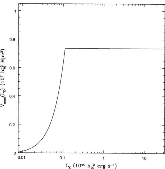
calculate Vm, [12]. Figure 6-1 shows the maximum volume probed by the R2FGS sample as a function of X-ray luminosity. I calculate Vm, assuming a flat •m, = 0.3 cosmology. Note that this assumption should not affect the final results significantly due to the local nature of the R2FGS sample.

0.8 S0.6 0.2 0 "• _E 0.4 0.2 03 0.01 0.1 1 10

L

(1044 h-•

erg

s-1)

Figure 6-1: The maximum volume sampled by R2FGS as a function of X-ray lumi-nosity.

6.1

Uniform Correction

As mentioned in §4.4, the reduced R2FGS sample introduces an incompleteness that must be accounted for when computing the mass function. The simplest possibility is to include a correction factor in Eq. (6.1):

dn(M)

1

E

1

(6.3)

dloglo M d

loglo

M

KVmax(Lx,i)'

where K = Nred/Ntot, that is, the number of systems included in the reduced sample

divided by the total number of systems in the original sample. Based on the analysis in §4.4, K = 45/62. This correction re-scales the mass function in a uniform manner by assuming that the incompleteness in the sample is distributed uniformly over all of the mass bins.

Figure 6-2 presents the R2FGS mass function computed using the virial masses from §4.2 and this correction; the results are discussed in more detail in §6.3.

6.2

Luminosity-Dependent Correction

Although the uniform correction discussed in the previous section is the simplest method of accounting for the incompleteness in the reduced R2FGS sample, it is not necessarily the most robust. Thus, I also consider a luminosity-dependent correction, which consists of the following steps:

1. Calibrate the M20 0 - Lx and U200 - Lx relations using the reduced R2FGS

sample, as given in Eqs. (5.3) and (5.2), respectively;

2. Calculate the X-ray luminosity of each system in the entire R2FGS sample from the X-ray flux according to:

Lx =

47fxd

(

-3 4--4 O_U 0 C) -5 0 ~ 6 -7 13.5 14 14.5 15

M

oo (h-

M

)

Figure 6-2: The R2FGS mass function (thick solid line), computed using a uniform correction applied to the virial masses of the reduced sample. The thick dash-dotted lines show the mass functions computed using the cosmological parameters from the WMAP1 results (upper) and WMAP3 results (lower), following the results of Jenkins et al [94]. The dashed (curved) line shows the best-fit mass function for the CIRS virial mass function; the unfit CIRS virial mass function is displayed by the dashed (straight) lines [28]. The light dotted line and error bars show the CIRS virial mass function computed after removing the minimum redshift and including all possible mergers as separate systems. This demonstrates the importance of cosmic variance at these low masses. The vertical line indicates the minimum mass I use to constrain cosmological parameters, although I do not perform that calculation for this mass function.

where dL is the luminosity distance to the cluster and z- is the mean value of

cz calculated from the redshifts of the member galaxies;

3. Insert these X-ray luminosities into Eqs. (5.3) and (5.2) in order to calculate

M200 and U200 for each system in the original R2FGS sample.

Note that in Step (2), I do not simply use the X-ray luminosities from Table 1 of Appendix B because these observational values are not as accurate as those com-puted from the observed X-ray fluxes according to Eq. (6.4). Also, note that in this luminosity-dependent correction, I utilize the resulting mass and velocity dispersion

estimates for all 62 of the original R2FGS systems in order to compute the mass function. The mass estimates are listed in Table 2 of Appendix B under the column

heading "MLx".

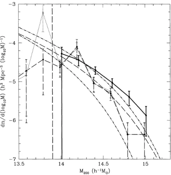
-Figure 6-3 presents the R2FGS mass function computed using these MLx and

U200,Lx estimates; the results are discussed in more detail in §6.3. In addition, I use

this mass function to constrain Qm and as8 in the next chapter.

6.3

Comparison to Previous Mass Functions

The original formalism for computing the mass function was based on Press-Schechter theory [1]. However, numerical simulations have predicted comparatively more mas-sive systems and fewer less masmas-sive systems than the Press-Schechter formalism [95]. Jenkins et al. calculated fitting formulae for a universal mass function that can be evaluated for a variety of cosmological models [94]. In fact, their mass function ac-curately replicates the mass function of dark matter halos in the Hubble Volume simulation. In recent years, many investigators have concluded that the following equation from Jenkins et al. [94] provides a nearly universal mass function, so that it can be used to constrain cosmological parameters [96]:

-3 O O _-4 0 5 C) 0 6 N~-6 13.5 14 14.5 15 M200 (h-IM®)

Figure 6-3: The R2FGS mass function (thick solid line), computed from masses found using the M - Lx relation calibrated with the reduced sample. The thick dash-dotted

lines show the mass functions computed using the cosmological parameters from the WMAP1 results (upper) and WMAP3 results (lower), following the results of Jenkins et al [94]. The dashed (curved) line shows the best-fit mass function for the CIRS virial mass function; the unfit CIRS virial mass function is displayed by the dashed (straight) lines [28]. The light dotted line and error bars show the CIRS virial mass function computed after removing the minimum redshift and including all possible mergers as separate systems. This demonstrates the importance of cosmic variance at these low masses. The vertical line indicates the minimum mass I use to constrain cosmological parameters in §7.