Centaur shapes and the origin of bilobate Jupiter-family comets

by Taylor K. Safrit

B.S. Earth, Atmospheric, and Planetary Sciences Massachusetts Institute of Technology, 2018

SUBMITTED TO THE DEPARTMENT OF EARTH, ATMOSPHERIC, AND PLANETARY SCIENCES IN PARTIAL FULFILLMENT OF THE REQUIREMENTS FOR THE DEGREE

OF

MASTER OF SCIENCE IN EARTH, ATMOSPHERIC, AND PLANETARY SCIENCES AT THE

MASSACHUSETTS INSTITUTE OF TECHNOLOGY MAY 2020

©2020 Taylor K. Safrit. All rights reserved.

The author hereby grants to MIT permission to reproduce and to distribute publicly paper and electronic copies of this thesis document in whole or in part

in any medium now known or hereafter created.

Signature of Author: ___________________________________________________________ Department of Earth, Atmospheric, and Planetary Sciences May 22, 2020 Certified by: __________________________________________________________________ Amanda Bosh Senior Lecturer Thesis Supervisor Accepted by:__________________________________________________________________

Robert van der Hilst Schlumberger Professor of Earth and Planetary Sciences Head of Department

by Taylor K. Safrit

Submitted to the Department of Earth, Atmospheric, and Planetary Sciences on May 22, 2020 in Partial Fulfillment of the Requirements for the Degree of

Master of Science in Earth, Atmospheric, and Planetary Sciences

ABSTRACT

The bilobate shape distribution of Jupiter-family comets (JFCs) is of unconstrained origin. One theory is that JFC progenitors become bilobate in the Centaur region, where sublimation of volatiles from object surfaces may spin objects up beyond a critical limit and disrupt them. We examine models of rotational body stresses to learn about this disruption. We also present new observations of four Centaurs in an effort to further constrain the shape distribution of the Centaur population. Of these four, insufficient data were gathered for three (2014 KR101, 2013 TC146, and 2013 XZ8). The fourth (2014 QA43) is shown to have a rotational period of 11.558 hours and is at minimum 11.5% elongated. This is not commensurate with a bilobate shape; there remain no known bilobate Centaurs.

Thesis Supervisor: Amanda Bosh Title: Senior Lecturer

Introduction

Observational data have shown that Solar System bodies can be broadly divided into a few shape classes. Large, self-gravitating bodies (i.e. planets, some moons, and large asteroids) are typically spheroidal with some oblateness derived from their rotation. Smaller bodies are often observed to be significantly more elongated in shape and are generally classified as triaxial ellipsoids3_{. A third shape class is known as bilobate or} contact binary objects: those objects which closely resemble (and are often thought to have been formed by) the aggregation of two spheroidal or ellipsoidal lobes of matter which are generally connected by a narrow neck. Prominent examples of this shape class include comet 67P/Churyumov-Gerasimenko, observed by the Rosetta

spacecraft and its Philae lander in 20144_{, and Kuiper belt object Arrokoth (2014 MU69),} observed by the New Horizons spacecraft in 20195_.

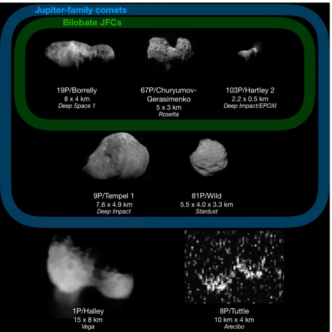
Over the past few decades, space missions have made close encounters with several Solar System comets4,6–11_{. Capable of observing these comets with resolution not} currently available from Earth- or near-Earth orbit-based instruments, these missions have given us our best data on cometary sizes, surfaces, and shapes. Notably, a large fraction of the cometary population that has been observed at such high resolution appears to consist of bilobate comets. Figure 1 shows all known shapes of comets in order to illustrate this.

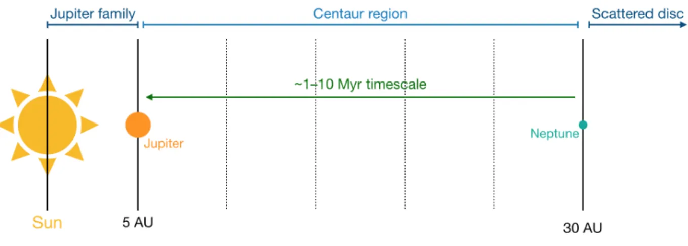
The process by which these bilobate comets are shaped is an unsolved problem. Several hypotheses have been investigated, from collisional catastrophic and sub-catastrophic disruption12,13 _{to binary accretion}14_{. One such investigation, detailed in our} recent paper1_{, considers whether bilobate Jupiter-family comets could be acquiring} their shapes in the Centaur region. The Centaur region is usually defined as lying between 5 and 30 AU, or roughly within the orbits of the giant planets, and consisting of objects (Centaurs) with both perihelion and aphelion within that range15_{. These} objects originate in the scattered disc, a collection of orbits with widely ranging values of eccentricity and inclination which are believed to have been scattered by encounters with the giant planets16_{. Objects are perturbed from the scattered disc into the Centaur} region by the outer giant planets, and generally spend 1-10 million years as Centaurs before being further perturbed inward or outward by any of the giant planets. Jupiter-family comets (JFCs) are the product of Centaurs which are perturbed into the Jupiter family by the gravitational influence of Jupiter16_{. These regions are detailed in Figure 2.}

Figure 1: Comets with known shapes and dimensions (from Safrit et al. 2020, in prep.).

Of the seven cometary nuclei for which we have high-resolution images, five are

bilobate. Comets 8P/Tuttle and 1P/Halley are classified as Halley-family comets ( highly thermally and dynamically evolved isotropic comets), rather than JFCs (evolved

scattered disc objects under the dynamical influence of Jupiter). 8P/Tuttle was observed as bilobate by the Arecibo radio telescope; the rest of these nuclei were observed by spacecraft. While detailed three-dimensional shape models do not exist for 19P/Borrelly and 1P/Halley, spacecraft observations suggest that they have bilobate shapes. Comets 9P/Tempel 1 and 81P/Wild are JFCs that are not observed to be bilobate (each has an oblate nucleus that is not considered elongated).

A Primordial Origin?

It is possible that bilobate JFCs are the result of a primordially bilobate scattered disc source population. If this is the case, we should expect to find a similar distribution of shapes in each of the populations that are dynamical precursors to the Jupiter family— Centaurs and scattered disc objects (SDOs). One potentially relevant object to this work is 2014 MU69 (Arrokoth), the subject of a 2019 New Horizons flyby. Arrokoth is a bilobate cold classical Kuiper belt object (KBO)5_{, part of a collection of objects with low} eccentricity and not governed by a resonance with Neptune. While it is not part of the source population of JFCs (the scattered disc is generally beyond the outer edge of the Kuiper belt), its shape closely resembles that of a bilobate JFC5_{. Arrokoth is thought to} be a contact binary resulting from a low-velocity (accretional) collision, rather than a body evolved by disruption or catastrophic collision5_{, and can be considered}

primordially bilobate in the scope of this work. Indeed, up to half of cold classical KBOs may be bilobate based on ground-based photometric observations17_{. If the} shape distribution of SDOs resembles the shape distribution of these cold classical KBOs (perhaps bilobate objects formed prior to the dynamical perturbations that separated the Kuiper belt and scattered disc), we should expect to see at least that many bilobate Centaurs; indeed, if bilobate JFCs are the end result of a bilobate source, we should expect the shape distributions of each of the Centaur region and scattered disc to be similar. However, no bilobate Centaurs have been observed, and without any real constraints on the shape distribution of the scattered disc, it is

impossible to say whether this is simply the result of small-number statistics (less than 20 Centaurs have rotational light curves in the literature) or proof that bilobate objects were not formed primordially.

Figure 2: Relevant regions of the Solar System.

Objects migrate inward from the scattered disc and spend ~1–10 million years in the Centaur region before being perturbed either back out of the Centaur region (or the Solar System entirely) or into the Jupiter family of comets. Sublimation of various volatile ices from the surface of bodies begins to turn on in the Centaur region.

Sublimative Torques

In the Centaur region, various volatiles actively sublimate from the surface of bodies18_. As examples, carbon monoxide begins to sublimate at heliocentric distances less than about 120 AU and so is active throughout the Centaur region, while CO2 sublimation is active at heliocentric distances less than about 13 AU18_{. The release of a sublimated} gas particle from the surface of a body induces a small force on the body; when the overall sublimation from a body’s surface is not perfectly isotropic, as is the case with an irregular body or one with only a few zones of active sublimation, the body therefore experiences a net torque. In Safrit et al. 2020, we asserted that Centaurs could

experience sufficient spin state changes as the result of this sublimative torqueing to spin up past a critical angular velocity (which depends on the cohesive or gravitational strength of the body) and be disrupted. This process depends on the properties of the sublimating volatile as well as the magnitude of an empirically determined sublimative coefficient (Cs), which accounts for shape, spin pole orientation and obliquity, and volatile distribution across the surface of a body†_{. We pointed to earlier work that} shows that bodies with typical cometary properties may, when disrupted, reform in bilobate shapes19,20_{. By modeling angular acceleration due to sublimative torques, we} calculated a set of possible upper bounds on the size at which disruption due to sublimation can no longer occur due to increasing gravitational binding of these

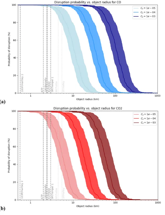
bodies, as well as a set of probabilities of disruption as a function of object radius, bulk density, and Cs. These probabilities are plotted in Figure 3.

† _{Larger values of Cs indicate a higher contribution of sublimation to angular acceleration. The range of} values used in Safrit et al. 2020 and shown in Figure 3 is derived from observed spin state changes of JFCs from the literature.

(a)

(b)

Figure 3: Probability of disruption as a function of object radius for CO/CO2 sublimation (from Safrit et al. 2020, in prep.).

For typical cometary sizes, computed probabilities of disruption are high for even the weakest combinations of sublimating volatile and sublimative coefficient !_!. CO sublimates over the full Centaur region, while CO2 sublimation is turned on within around 13 AU. Figure

3a shows probabilities for CO, while Figure 3b shows probabilities for CO2. Each area

corresponds to the probability of disruption as a function of radius for the indicated !_! and a range of densities: the low edge corresponds to a body bulk density of 700 kg/m3_{, the line}

through the area corresponds to a body bulk density of 500 kg/m3_{, and the upper edge}

If sublimative processes are indeed shaping objects in the Centaur region, we would expect to see some Centaurs which have undergone disruption and reformed, potentially in bilobate shapes. In this scenario, the scattered disc would not be

primordially bilobate, so we would expect to find a smaller fraction of bilobate Centaurs than we do of bilobate JFCs. However, it is challenging to constrain the ratio of

bilobate to non-bilobate Centaurs that we should expect to see. While we would expect to find non-bilobate Centaurs in the process of spinning up before being

disrupted, angular acceleration from sublimative torqueing is a stochastic process, and could be alternately spinning up and spinning down the same body, depending on the shift of active zones1_{. And while recent work produced an empirical coefficient of} sublimation Cs from the known spin state changes of JFCs14 _{(which should account for} the above stochasticity), there is some unknown upper bound on object radius beyond which disruption no longer results in bilobate formation.

Modeling

Sublimative coefficient

In support of two of our recent papers, we used observations of the changes in rotation period of several Jupiter-family comets to empirically constrain the sublimative

coefficient Cs, a key scaling factor in our sublimative torqueing model1,14,21_{. Cs accounts} for shape, spin pole orientation and obliquity, and volatile distribution across the

surface of a body, which are not easy to constrain for a wide set of bodies: different comets have different shapes, orientations, and distributions of volatiles. By

incorporating the known rotation rate changes of JFCs, our new range of Cs values accounted for the natural variation in these quantities. We found Cs for these JFCs to span only around one order of magnitude, from 10-5 _{to 10}-4_{, assuming only water ice} was sublimating. While this was smaller than our previous estimate of 10-3 _(for

Centaurs, rather than JFCs), we found that the probabilities of disruption for JFC-sized bodies remained high when our model was run with this range of Cs values.

Stresses on a rotating body

Hirabayashi presented a model of stresses on a rotating body due to spin-up in a 2015 paper focused on asteroid disruption22_{. He found that, intuitively, the stresses caused} by rotation on a spherical body are highest in the material furthest from the rotation axis, and can result in increased oblateness or full disruption of an object under certain conditions.

We created a simple model of stresses on a rotating solid body to determine the radial strain that should be experienced by a Centaur undergoing sublimative torqueing. To determine the stress at a given point in a rotating body, we treated the body as ellipsoidal and composed of a number of small discs (stacked concentrically) rotating about their centers. For demonstration, we chose a spherical body with radius 1 km, for which gravitational self-attraction is negligible compared to body cohesion. These simplifications allowed us to make the approximation that the radial stress at a

distance ! from the center of each disc is " = (!"_#!)(3 + ()()$_{− !}$_),23 _{where + is the} body’s density, , is the body’s angular frequency, ( is the material’s Poisson ratio (0.5 for incompressible materials) and ) is the outer radius of that disc. We treated the body as composed of solid CO2 ice with a density of 1500 kg/m3 _{and a tensile strength} of 1.5 MPa (approximated, based on water ice)24,25_{. We used an observed relation} between CO2 ice temperature and its Young’s modulus, - = −1.361 × 10% ₄$₊

2.985 × 10& _{4 + 1.47 × 10}'( _{Pa, where T is the temperature in Kelvins}26_{, and set the} temperature to be 65 K, which is effective temperature at 20 AU from the Sun18_{. At this} temperature, the first two terms are negligible, so - = 1.47 × 10'( _{Pa. We modeled our}

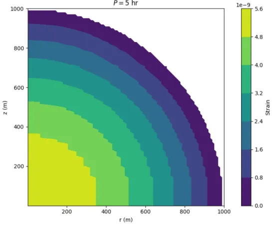
icy body as a Bingham viscoplastic, which acts as a linear elastic material until its cohesion is overcome by stress. Our first result, assuming linear elasticity, calculated a strain in the radial direction ; = "/- for each disc, and thereby for the body as a whole. The result is shown in Figure 4 for a spherical body with a rotational period of 5 hours.

We found a maximum strain of less than 6 × 10)* _{near the center of the body. This}

strain is negligible, resulting in effectively 0 elongation in the linear elastic regime. Our modeled stresses were order ~10–100 Pa, multiple orders of magnitude less than the

Figure 4: Strain on rotating body with 5-hour rotational period.

Our maximum modeled strain on a 1-kilometer-radius body is less than 6 × 10"#_{, near the} center. This results in effectively 0 elongation; pure ice is not an appropriate approximation for a rubble-pile-like comet or Centaur. For bodies with longer periods, these strains are smaller.

tensile strength of our body. The modeled Bingham-viscoplastic body did not therefore approach plasticity, and would not even for much larger values of ,. Our model of pure CO2 ice thus shows it to not be a particularly appropriate analog for the rubble-pile-like composition of a typical comet or Centaur. A Centaur with exceedingly low porosity might be better approximated by this low-elongation result.

Observations

This principal goal of this observational study was to determine the shapes of the set of Centaurs that we observed. This would allow us to flesh out our knowledge of the Centaur region and potentially make conjectures about both the origin of the shape distribution in JFCs and the shape distribution of SDOs. As we were limited to ground-based observing and had a reasonably small time window, the best option for

determining shapes was collecting high-resolution light curves for a set of Centaurs and examining the contours of the light curves. Assuming the observed object to be a triaxial ellipsoid with axes a, b, and c and rotating about its axis c, the difference between flux collected at the crest and trough of a sinusoidal light curve can be used to determine the ratio of the other two axes a and b. Each observed object could be in any possible viewing aspect; it is possible that objects we observe are rotating such that the same surface area is presented to Earth-based observers at all times. In our calculations, we assume that the axis of rotation is in the sky plane of the observer, so the object rotates between minimum and maximum reflected surface area.

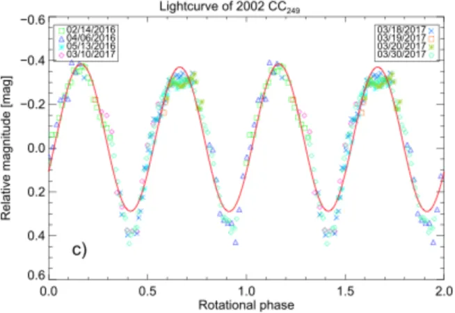
Calculated axis ratios should therefore be treated as a lower limit on object elongation High enough temporal resolution (combined with high enough light curve resolution) can allow us to make a conjecture about the potential bilobate nature of an object. Bilobate objects, including contact binaries, have a characteristically “U/V”-shaped light curve, in which crests are rounded while troughs are more sharply peaked2_{. An} example of such a light curve is shown in Figure 5, reproduced from Thirouin and Sheppard 20172_{. The discrepancy in crest and trough shapes is due to shadowing and} viewing geometry effects observed when viewing a bilobate object nearly equator-on and at low phase angle.

Our observations were carried out between 2019 September 25 to 2020 January 14 between telescopes at Las Campanas Observatory in Chile and Lowell Observatory in the United States (Arizona). Telescopes used are summarized in Table 1a; objects observed are summarized in Table 1b; data collected are summarized in Table 1c. At Las Campanas, we received 1.5 nights on the Clay telescope on 25 and 26 September; at Lowell, we received 3 nights on the Lowell Discovery Telescope, of which two were clouded out (leaving 14 January as the sole clear session). These data were

supplemented by data from Las Cumbres Observatory, which consisted of two partial nights on 1-meter-class telescopes in South Africa and Chile. We observed with the Sloan r’ filter.

Figure 5: Light curve of bilobate-candidate cold classical 2002 CC249 (from Thirouin and Sheppard 2017).

Note the discrepancy in shape between peaks and troughs in this light curve. This characteristic “U/V” shape occurs due to shadowing and viewing geometry effects

observed when viewing the rotation of a bilobate object nearly equator-on and at low phase angle.

O b se rv at or y Lo cat ion T el es cop e Ap er tu re (m ) In st ru m en t F ie ld w id th (ar cm in .) Las C am p an as O b se rv at or y A tac am a, C h il e M age ll an — C la y 6. 5 LD S S -3 6. 4 Lo w el l O b se rv at or y F lags ta ↵ , AZ , US A Lo w el l D is co ve ry T el es cop e 4. 3 LM I 12. 5 Las C u m b re s O b se rv at or y C ap e T ow n , S ou th Af ri ca LC O G T 1m 1 S in is tr o 26 Las C u m b re s O b se rv at or y C er ro T ol ol o, A tac am a, C h il e LC O G T 1m 1 S in is tr o 13 (b in n ed 2x 2) <latexit sha1_base64="eUW03uCUBoowLqq8fMxH7BVnwwo=">AAAEHHicfVPLbhMxFJ0mPEp4tbCEhaECpVISZdK0sGxIVaiUqkVJ2opOVN3xOIlVjz2yPW3CKCv+gz1b+AV2iC0Sf8BncGcaoSYFPPLo+Pr6nPuw/UhwY6vVnwu5/LXrN24u3ircvnP33v2l5QcHRsWasi5VQukjHwwTXLKu5Vawo0gzCH3BDv3TZrp/eMa04Up27DhivRAGkvc5BYumk+XcY08zw98zX40Sz7KRPeeBHU6SJ5Ok4PlswGViwY8F6ElC6KVvUvCGqWphzzdMn4FVekyek5a6oEbYYYIZqiKGuBExbWPNSDFcxeWONFbHIZMWF9uciYBkuqQImoZcVlY9b8pPCi0wpAlhBBLBrFrDAoUQSqQ55CLV2YUBEwIkKZfLpCkgddqorKeBbbXb5bVsWSfI3lLn6DnHty1gYCz0+yXSeFci3XYjSynz3OKYDNZyPJNYvZJytnZ38O/WUCmlTgOOQx8rO8ffBDzUUeeyRNoqxnwbfY29SBmae687xA1TGpxtLrH5WiGsbfyfkml062CnhSpdLci/ed01UvS5lCwgtVFtNQ3cYzL40+7CpHCytFKtVLNBrgJ3Clac6dg/WfrlBYpmjaUCjDl2q5HtJaAtp4LhlYkNi4CeYpeOEUoImekl2TWekGdoCUhfaZx4MTLr5RMJhMaMQx89Q7BDM7+XGv+2dxzb/stewmUUWybphVA/FsQqkr4JEnDNqBVjBEA1x1gJHYIGavHlzKgMNERDTkdZadz5QlwFB7WKW6+sv62vbL6aFmnReeQ8dYqO67xwNp03zr7TdWjuQ+5T7nPuS/5j/mv+W/77hWtuYXrmoTMz8j9+A1YDRAE=</latexit>

O

b

je

ct

S

em

im

a

jor

ax

is

(A

U)

E

cc

en

tr

ic

it

y

In

cl

in

at

ion

(d

eg.

)

H

(m

ag)

D

iam

.

(k

m

,

fr

om

H)

2014

K

R

101

14.

775

0.

284

9.

122

11.

2

27.

4

2013

T

C

146

25.

382

0.

163

14.

173

6.

5

238.

5

2013

XZ

8

13.

417

0.

372

22.

534

9.

5

59.

9

2014

Q

A43

9

.653

0.

506

37.

214

11.

4

25.

0

<latexit sha1_base64="62M0uaLRc8SQhbqxZx8gwiN7mhQ=">AAADjnicbVLbbhMxEN0kXMpyS+GxL4ZQlErIWu8lmzwgWgpSEA+00LRRs1HkdZzEzd5keyFhlV/g//gDfoB37E1AveB9mOOZOXNmxxNmERPSsn5WqrVbt+/c3bpn3n/w8NHj+vaTU5HmnNAeSaOU90MsaMQS2pNMRrSfcYrjMKJn4fxQx8++Ui5YmpzIZUaHMZ4mbMIIlso12q78CDgV7DsN00URSLqQ39hYzlbFs1VhBiGdsqSQOMwjzFcFIJe+lRnMtKr5KbygRIKX4AuNWYwvUg7wggnQPOjtKe97QmgiOSNMLtX1Q0IUq1QHzTGdQp3TBU3Vl0bvGI4haM7jV2DC0xh090AQbJSAaVvIBR8/IwupVORC3/cUsKDddpXtQGTbOoCgNrYPXU1WJAecHCK3pZ0edNp2SUItZ10F+Rq0oK5lO21l/7L6522d4kAX+SXH8cvKNvSctaLmeB3Y2VBccHzgOmWk5TklxbO0ruNDG7nr5tx1H1b5ZzQZ/xuwuTJH9YYFrfKAmwBtQMPYnKNR/VcwTkkeqxmTCAsxQFYmhwXmkpGIqkfKBc0wmeMpHSiY4JiKYVEuzgrsKs8YTNSLTdJEgtJ7mVHgWIhlHKrMGMuZuB7Tzv/FBrmctIcFS7Jc0oSshSZ5BGQK9BaCMeNqZ6KlAphwpnoFZIY5JlLt6hWVKcfZjJFFORp0fRA3wakN1ZN6x25j/+1mSFvGjvHcaBrI8I19o2scGT2DVH5Xd6ovqru1eq1Ve117s06tVjacp8aVU+v+Ae0m+Ps=</latexit> O b je ct D at e (UT C ) He li o ce n tr ic d is tan ce (au ) P h as e an gl e (d eg. ) T el es cop e # fr am es E x p os u re ti m e (s ) C om m en ts 2014 Q A43 2019- 09-25 4. 9123 9. 7614 C la y 16 300 P o or se ei n g 2014 Q A43 2019- 09-26 4. 9136 9. 6944 C la y 412 30 2014 Q A43 2019- 11-19 4. 9947 8. 5432 LC O G T -C P T 14 600 2014 Q A43 2019- 11-20 4. 9964 8. 5867 LC O G T -LS C 8 600 2014 Q A43 2020- 01-14 5. 0947 11. 0353 LD T 31 300 2014 K R 101 2019- 09-25 10. 7579 4. 5472 C la y 31 300 P o or se ei n g 2013 T C 146 2019- 09-26 26. 9257 1. 3558 C la y 120 60 89 u sab le fr am es 2013 XZ 8 2020- 01-14 8. 5953 6. 0999 LD T 31 300 <latexit sha1_base64="nRPxkiCe1DGa2cbTo3rk7rYba5o=">AAAFEnicfVTLbtNAFHVJgBJebVmyGYhAZRFrxq/Eu0KKqESltpA+RB1V48kkMfVLnjE0WPkL9mzhF9ghtvwAf8BncMcJJU0oY8m+vo8z5x7fsZ+GgZAY/1y6UqlevXZ9+Ubt5q3bd+6urK4diCTPGN9nSZhkRz4VPAxivi8DGfKjNOM08kN+6J+2VfzwHc9EkMQdOUp5N6KDOOgHjEpwnaxW1ryMi+AD95OzwpP8TL4PenI4Lh6Mi5rn80EQF5L6eUizcYHYwjWueUO1d23Hf8uZRI/RJpUcre932k/gZQuIJYzHMgsY6kE7NGYQpbkK7g6BOKLxIARXjw905ezwkAuWpBxsr476GY24APv5WZqIPONIBhGkC5XbTqIIsAXyvCkNVDMwsdDeU8uEONhuA7sNw4YXS3eJobyu3nQgB8pDOoIHceBmYqwYJUmGBOdBPPC8S7CcKZbplFiOa81gWcQowRR5b7GekAZxJ/Wu1QSjpduWqUq22zsvOo32bkcRUoAO/g+IgacgjjUBaTnNc5Dt123lvBzDwA0MRFSpreMJEUJ0bNoqvr2pOJjkXJQ/9S9fEUzmVSVYb9rNSU+21TT+SjGDsCiriTptYjnzuhqO7hp2yUc3bbs185HKlh11a7koFxQGfDocE34mOnrTmm8PlHHLphzo03Uv6c7jce98yGvj2slKHeu4XGjRIFOjrk3X7snKL6+XsFzNIgupEMcEp7Jb0EwGLORwRHLBU8pO6YAfgxkr1t2iPLxj9Ag8PdQHhfpJLFHpna0oaCTEKPIhM6JyKOZjyvmv2HEu+61uEcRpLnnMJhv18xDJBKk/ARzHDE5sOAKDsiwArogNaUaZhP/FhV0GGU2HATsrpSHzQiwaB4ZOYBz2jPrGs6lIy9p97aG2rhGtqW1oW9qutq+xyqjyqfK58qX6sfq1+q36fZJ6ZWlac0+7sKo/fgPAPlPI</latexit> Tabl e 1: O bs er vat ional par am et er s and dat a col lect ed Tel escope speci ficat ions ar e list ed in tabl e (a) ; r el evant obj ect par am et er s ar e list ed in tabl e (b) . Tabl e (c) gi ves al l dat a col lect ed dur ing our obser vat ional sur vey. (a) (b) (c)

Calibration

Data taken on LDSS-3 at the Clay telescope were flattened with twilight flats. Data taken on LMI at the Lowell Discovery Telescope were flattened with averaged twilight and dome flats. (Dome flats were taken on the night of 2020 January 14th_{, which was} otherwise clouded out.) LCOGT data were flattened automatically as part of the LCOGT programming. We used on-chip standard stars no more than half of the given field size separated from each target to calculate the apparent magnitude of the target Centaur in each frame of data. We retrieved these standard stars used, and their magnitudes in the r’ filter, from the APASS survey27 _{using the PMM Image and} Catalogue Archive Service22_{. We performed preliminary photometric analysis with} AstroImageJ. Representative frames of data, with comparison stars, are shown in the appendix.

In order to perform photometric analysis of Solar System bodies on elliptical orbits, it is necessary to standardize apparent magnitudes by scaling them with distance and phase angle (the angle between the Sun and the observer as viewed from the body). We used the following equations28 _{to calculate the absolute magnitude H of our target} for each frame of data, defined as the observed magnitude of an object at 1 AU from both the Sun and the observer and fully illuminated (0º phase angle):

=(>) = ? − 5log (!Δ)

= = =(>) + 2.5log [(1 − E)F_'(>) + EF_$(>)] for

F₊(>) = exp [−K₊Ltan' $⁄ _>P-"_]

Q = {1, 2}, K_' = 3.33, K_$ = 1.87, U_' = 0.63, U_$ = 1.22

where V is our observed magnitude, r is the heliocentric distance of the object, Δ is the distance between the object and Earth, > is the phase angle between the Sun, the object, and the Earth, and G is the slope parameter, which depends on the particular scattering of light by the surface of a body. For asteroids, G is typically assumed to be 0.15, which is the value used here. We retrieved distances and phase angles from JPL HORIZONS29 _{(see Table 1 for these values).}

2014 KR101

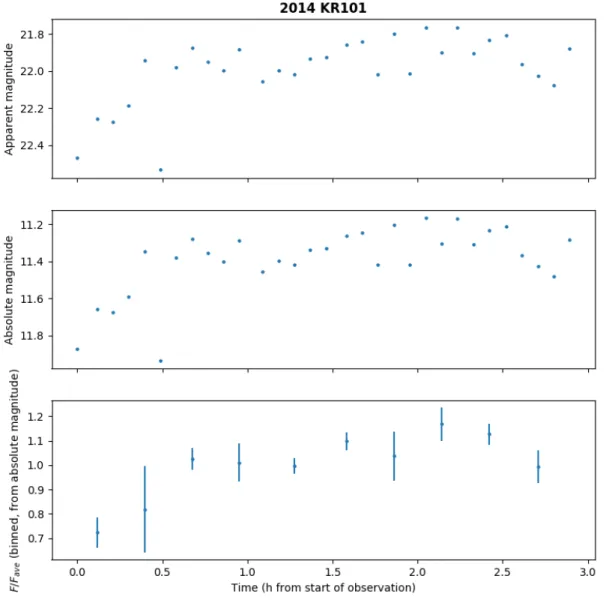
Our data for the Centaur 2014 KR101 span nearly 3 hours of observation. These data are quite noisy but appear to show a significant brightening of around 0.6 magnitudes in the first hour of observation. The relevant frames of data, and the results of the processing of these frames, do not show any errors that might account for this. The shape of the overall light curve is not likely to be physical; the shape of the light curve is not sinusoidal, and we do not suspect that this is the result of a sporadic event. In order to extract a useful metric from these data, we will analyze the maximum axis ratio that an elongated object could have from the truncated data set (without the first 30 minutes). We plot the mean and standard deviation of the scaled flux for each set of 3 points in Figure 6. Disregarding the first two bins, bin means range from 0.994 times

the average flux to 1.168 times the average flux. If the noisy data are masking a sinusoidal light curve (or part of one), we calculate a maximum surface area ratio of

'.'&#

(.**/ = 1.175 and a axis ratio 0

1 of √1.175 = 1.084.

Figure 6: Observations of 2014 KR101.

We plot each data point collected from 2014 KR101 on 2019 September 25 in apparent and absolute magnitude, as well as binned and scaled flux, against time in hours. There is a large increase in brightness in the first ~5 points that is unlikely to be the result of a physical phenomenon.

2013 TC146

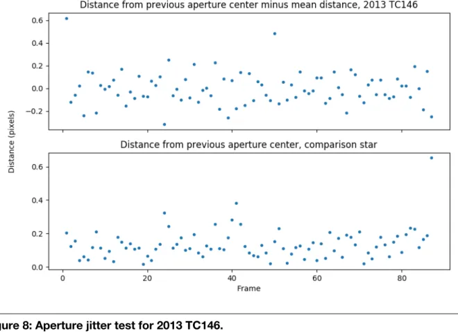
Of the 120 frames of data we collected of 2013 TC146, 89 were usable, as the Centaur began to overlap a galaxy on the chip starting with frame 90. Our data for 2013 TC146 (shown in Figure 7) show a spread of about 0.1 magnitude but which generally appears to be due to noise alone. When binned (with 7 data points per bin), the spread of bin means is less than 0.04 magnitudes. Note that some of the individual points (e.g. those around the 1-hour mark) appear to fluctuate between more and less signal in a more methodical way than pure noise would suggest. It is unclear whether this is in fact an artifact of our method of data processing or simply a particularly worrisome random noise signal. One hypothesis is that this fluctuation is due to “jittering” of the aperture centers for 2013 TC146 or our comparison star, which correspond to the centroid of the signal for each object in each frame. To test this hypothesis, we plot the aperture centers and their relative movement between frames in Figure 8. There is no obvious correlation between the movement of the aperture centers and the fluctuating noise observed in the magnitude signal; it is therefore likely that this fluctuation is random noise.

For the sake of completeness, we will calculate the potential axis ratios of 2013 TC146, treating the slight convex shape of the light curve as part of a sinusoid. The mean scaled flux of each bin of 7 data points varies between 0.983 and 1.011.

If we have observed a quarter period from inflection point to crest or a half period from inflection point to inflection point, we can calculate the scaled flux at the trough as 0.983 − (1.011 − 0.983) = 0.955. This leads to an surface area ratio of '.(''

(.*%%= 1.059 and

a axis ratio 0₁ of √1.059 = 1.029.

If we have observed a full period from trough to trough (which is quite unlikely as this would imply a rotation rate of less than 2.5 hours, significantly more rapid than the fastest-rotating known Centaur), we can calculate a surface area ratio of '.(''_(.*#2= 1.028 and a axis ratio 0₁ of √1.028 = 1.014.

Figure 7: Observations of 2013 TC146.

We plot each data point collected from 2013 TC146 on 2019 September 26 in apparent and absolute magnitude, as well as binned and scaled flux, against time in hours. These data do not appear to be sinusoidal. Note that some pairs of points around 1 hour appear to be fluctuating regularly between higher and lower flux; this is likely random noise that simply appears regular to the eye.

2013 XZ8

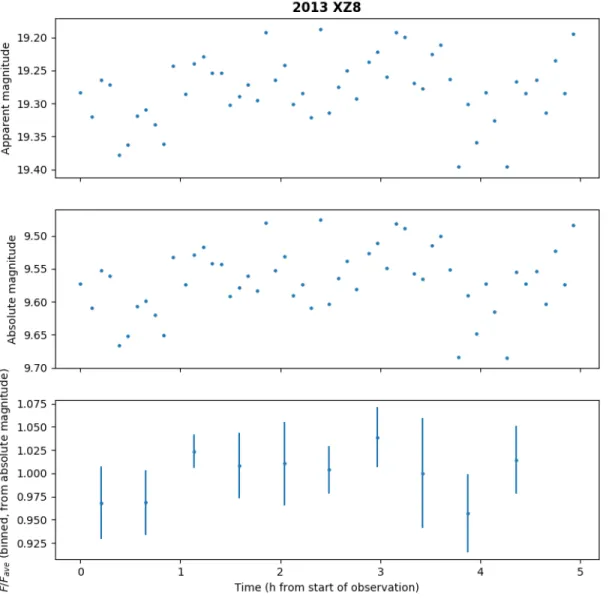
Our data for 2013 XZ8 show a magnitude spread of around 0.2 which is again apparently noise-dominated. The mean and standard deviation of the scaled flux for each set of 5 points are shown in Figure 9. The mean scaled fluxes range between 0.957 and 1.039. This data look very similar to our observations of 2013 TC146; again, for the sake of completeness, we repeat the above calculations.

If we have observed a quarter period from inflection point to crest or a half period from inflection point to inflection point, we can calculate the scaled flux at the trough as 0.957 − (1.039 − 0.987) = 0.875. This leads to an surface area ratio of '.(2*_(.#3%= 1.187 and a axis ratio 0₁ of √1.187 = 1.089.

If we have observed a full period from trough to trough, we can calculate a surface area ratio of '.(2*_(.*%3= 1.086 and a axis ratio 0₁ of √1.086 = 1.042.

Figure 8: Aperture jitter test for 2013 TC146.

In order to determine if the seemingly nonrandom fluctuations in the data series of 2013 TC146 are in fact nonrandom, we plot the “jitter” of each aperture as a function of frame number. If the pattern in the noise in Figure 7 were replicated here, it would be a sign that that pattern was caused by a problem with the aperture on 2013 TC146 or the comparison star. As this is not the case, it is likely that the pattern is in fact random.

Figure 19: Observations of 2013 XZ8.

We plot each data point collected from 2013 XZ8 on 2020 January 14 in apparent and absolute magnitude, as well as binned and scaled flux, against time in hours. These data are noisy and do not appear to be sinusoidal.

2014 QA43

Of our targets, by far the largest number of data points were collected observing the Centaur 2014 QA43. These data span three nights of in-person observing on large telescopes at Las Campanas and Lowell observatories as well as two nights of

remotely collected data from 1-meter-class telescopes associated with Las Cumbres Observatory. These data are presented in Figure 10 in apparent and absolute (as calculated above) magnitudes.

We used a Lomb-Scargle periodogram analysis, implemented with the Python module astropy, to find possible values of the period for 2014 QA43. We chose the Lomb-Scargle periodogram to best work with the extremely uneven sampling of our data points. The result of this analysis of our data for 2014 QA43 is shown in Figure 11. Note the lack of any sharp single peak.

Figure 10: Observations of 2014 QA43.

We plot each data point collected from 2014 QA43 across all observations in apparent and absolute magnitude. Note the importance of plotting in absolute magnitude; the viewing parameter change between observations resulted in a significant drop in apparent

brightness between September and January. Note also the spread and number of points for each set of observations, with by far the most data collected on 2019 September 25 (in orange).

Figure 12, which shows the phased result of this periodogram analysis, shows that none of the three highest peaks, at 5.779, 5.963, and 5.583 hour periods respectively, produces a definitive result. We will treat 5.779 hours as the best result, as it appears to match the two LCO-Clay curves most closely. Given the low points between peaks, which lie at periods of 5.884 and 5.654 hours, we can give a measurement with error of 5.779 (+0.105) (-0.125) hours for the half-period of 2014 QA43. Note that, as 2014 QA43 appears to be elongated, its true period will span two sinusoidal periods, the peaks of which correspond to one “side-on” view of the larger aspect of the Centaur. The true period of 2014 QA43 is therefore twice 5.779 hours, or 11.558 hours. In the following figures, however, we will phase our data by half-period for ease of analysis.

Figure 11: Lomb-Scargle periodogram from 2014 QA43 data.

Note the lack of any sharp peak; as the data are significantly separated in time and are slightly different in absolute magnitude, the best frequency is not definitively clear. The highest peak, at a period of 5.779 hours, is marked with the solid line; the two next highest peaks are marked with dashed lines, and the local minima between them are marked with dotted lines. We treat these local minima as the error on either side of the main peak.

We can produce a much sharper-peaked periodogram using the LCO data only, but the peak does not fit any data other than the two LCO dates. This result is shown for comparison in Figure 13.

Figure 12: Phased data, 2014 QA43.

We plot the scaled flux of 2014 QA43 against time, phased by each of the three highest peaks from Figure 11. Here the slight brightness drop between the observations in

September and those later becomes apparent. It is clear, however, that 5.779 hours is the best period, and that both a trough and crest were observed in the September data.

(a)

(b)

Figure 13: Periodogram (using only September data) and phased data, 2014 QA43

When we consider only the September data, we can create a Lomb-Scargle periodogram with a single prominent peak (a); however, using this peak to phase our data (as in Figure 12) reveals significant error (b).

There are a few reasons our data might not be correctly calibrated across nights. The comparison stars used were not linked across nights or instruments, which introduces some unknown error in our determined apparent magnitudes. It is possible that 2014 QA43 was observed during an outburst event that spanned 2019 September 25 and 26, but was not present during later observations: an outburst of volatile gas and dust particles could have increased the effective albedo of the body, or its effective surface area, and therefore the reflected brightness. This could explain what appear to be systematically dimmer data on the later observed dates, although those data are not perfectly uniform either. An unlikely possibility is that the observed body geometry changed enough to create this discrepancy between viewings—however, the change in phase angle was small from 2019 September 25 to 2020 January 14. And our assumed slope parameter of 0.15 could be causing our calculation of absolute magnitude to be inaccurate.

In light of the observed discrepancy, we will focus on the Las Campanas data for our remaining analysis in order to better constrain the parameters of 2014 QA43. We will continue to use the best determined half-period from the entire data set of 5.779 (+0.105) (-0.125) hours. The trough observed on 2019 September 25 is at absolute magnitude 11.557; the crest observed on 2019 September 25 is at absolute magnitude 11.321. This gives us an amplitude of 0.236 magnitudes for the 5.779-hour half-period. In brightness flux, the ratio between the scaled maximum and minimum (at the same crest and trough) is '.(#(_(.#&*= 1.243, which gives an axis ratio of √1.243 = 1.115.

This 11.5% elongation does not lend itself to the typical image of a bilobate object, in which two roughly-equal lobes rotate around an axis drawn through the narrow neck connecting them. However, we could be observing a bilobate 2014 QA43 from an unfavorable viewing aspect; that is, an orientation in which the full extent of its

elongation is not visible. To further investigate any possibility of a bilobate shape, we can examine the difference in width between the crest and trough shapes, as in

Thirouin and Sheppard 20172_{. In that work, the authors compute the full width half max} (FWHM) of Gaussians fitted to the crest and trough to compare the peak width.

Because our data are disjoint across nights and significantly more time is represented in our data from September 26, we instead fit sinusoids to each night of observation, assuming that the midpoint of the curve in flux is halfway between the maximum and minimum flux. (Comparing the periods of the sinusoids is equivalent to comparing the FWHM of fitted Gaussians). Figure 14 shows the data taken at Las Campanas

Observatory fitted in this way, and the periods of each sinusoid. Note that each fitted sinusoidal period is smaller than the assumed 5.779-hour period, as the half-period was calculated with all collected data.

There is a 28.3% difference between the periods of each sinusoid. Observed bilobate and contact binary candidates have crest FWHM/trough FWHM ratios of greater than about 50% due to shadowing and viewing geometry effects2_{. Thus, the 28.3%}

difference in fitted period is likely not representative of a bilobate shape.

Results and Discussion

Collected data are not high enough resolution to fit a sinusoidal light curve and

determine a shape for the Centaurs 2014 KR101, 2013 TC146, and 2013 XZ8. We can still place some constraints on the maximum axis ratios of these objects by operating under the assumptions that our collected data represent quarter, half, or whole periods and that these Centaurs are rotating around their short axes oriented on the sky plane (in an “optimal” viewing aspect); these constraints are summarized in Table 2. Among these objects, we do not find any with strong elongation (all have <10% elongation), and we can therefore conclude that none are bilobate. For the Centaur 2014 QA43, we

Figure 14: Fit differences between trough and crest, 2014 QA43.

In order to determine if 2014 QA43 is bilobate, we examine the shape of the trough and crest by fitting sinusoids to each set of data. The sinusoid fitted to the September 25 data has a period of 4.167 hours, while the sinusoid fitted to the September 26 data has a period of 5.346 hours, a 28.3% increase. This is small compared to the observed ~50% increase in FWHM between trough and crest of bilobate Kuiper belt objects as in Thirouin and

Safrit 25 have a larger set of higher-quality data, which is strongly periodic with a full period of 11.558 hours and an amplitude of 0.236 magnitudes, which suggests a maximum axis ratio (under the above assumptions) of 1.115.

2014 QA43 is likely not bilobate either—an axis ratio of 1.115 does not imply a bilobate shape (subject to viewing aspect assumptions), and while the Centaur may have been viewed in a non-face-on orientation, the 28% difference in fitted period between the crest and the trough is small compared to that observed in previous work2_{. The} observed difference may still suggest shadowing or other viewing geometry effects that appear in the trough (when the smallest surface area faces the observer). We are able to place 2014 QA43 into the set of Centaurs with known rotation periods29,30_{, and show this result in Figure 15. As we continue to learn about the} Centaur population, this set will continue to expand. There are a large number of

variables at work here; as such, it is fundamentally difficult to separate them in order to glean information about formation mechanisms. Notably, none of the bodies plotted have been observed to be bilobate.

Object

Axis ratio a/b if...

...quarter or half period observed

...full period observed

2014 KR101

1.084

1.084

2013 TC146

1.029

1.014

2013 XZ8

1.089

1.042

2014 QA43

—

1.115

Table 2: Determined axis ratios, assuming portion of period observed.

For the objects with incomplete periods in our data set, we can calculate the maximum axis ratio under a set of assumptions: that the Centaurs observed have their rotation axes aligned with their shortest axis c and in the plane of the sky, and that the observed

variations are due to inherent object geometry rather than noise in our data. For 2014 QA43, we can calculate a lower limit on axis ratio of 1.115 under the same set of assumptions (which represent a full minimum–maximum reflected area cycle).

The lack of bilobate Centaurs in our data set, and the overall Centaur population, may be indicative of the shape distribution among different populations in the Solar System. If the bilobate shapes of JFCs were the result of a primordial, bilobate scattered disc population, we would expect to see a similar proportion of bilobate objects in our study of Centaurs—2 or 3 out of the 4 observed. Because we find instead 0 out of 4, we can be more confident that objects become bilobate after being perturbed out of the scattered disc. This might happen in the Centaur region, where sublimative torqueing could play a large role in the rotation state changes of objects and their eventual disruption; it might happen in the Jupiter-family, where significant sublimative rotation state changes have been observed in comets.

Of course, we are firmly in the regime of small-number statistics. Further work in constraining the shape distributions in the scattered disc, Centaur region, and Jupiter family is needed to learn more about the mechanism for the formation of the

Figure 15: Centaurs with constrained rotation periods, including 2014 QA43.

All Centaurs with known rotation periods are plotted against their semimajor axes. Increasing point size corresponds to increasing diameter (calculated with H magnitude, assuming an average Centaur albedo of 0.078, where diameter is not yet constrained). Color corresponds to perihelion distance. There is generally no observed trend; most, but not all, Centaurs have rotation rates under around 10 hours. The rotation rate of 2014 QA43 is somewhat slow in comparison, while the Centaur itself is small and located in the inner part of the Centaur region.

distribution. This could be modeling work, in which more sophisticated, soft-sphere hydrodynamic models are used to approximate the mechanics of rubble piles19_{: while} our presented model predicts some elongation as the result of rotational stresses, the elongation is very small even at high rotational velocities.

Beyond further photometric observation, occultation observations are a viable method of constraining these shape distributions: occultation studies have successfully

produced some of the most detailed models of Centaurs to date. A 2013 occultation of the Centaur Chariklo revealed two rings orbiting its nucleus31_{. While sublimating}

volatiles are unlikely to be involved in ring production, the level of shape resolution demonstrated by this occultation (rings of 3 and 7 kilometer widths 9 km from a 250-kilometer-diameter object) would be quite sufficient to detect a bilobate shape,

provided the object occulting is viewed side-on and at least three chords with sufficient time and spatial resolution are observed. Of course this is a nontrivial requirement, but the resolution afforded by occultation data could be put to good use in the study of Centaur shapes.

Conclusion

None of the Centaurs in our observational study appear to be bilobate. 2014 QA43, of which the most and best data were collected, is shown to have a 11.558-hour period with a minimum elongation of 11.5%, assuming an optimal viewing aspect. The other Centaurs observed have maximum elongations which are all under 10%, assuming an optimal viewing aspect. There continue to be no observed bilobate Centaurs. This is likely a product of the small sample size of Centaurs with high-resolution light curves, but may indicate that SDOs, the source population of Centaurs and thereby JFCs, are not primordially bilobate. Further models and observations are required to place better constraints on the shape distributions of these populations.

References

1. Safrit, T. K. et al. The Formation of Bilobate Comet Shapes through Sublimative Torques. (2020).

2. Thirouin, A. & Sheppard, S. S. A Possible Dynamically Cold Classical Contact Binary: (126719) 2002 CC 249. AJ 154, 241 (2017).

3. Scheeres, D. J. Dynamics about Uniformly Rotating Triaxial Ellipsoids: Applications to Asteroids. Icarus 110, 225–238 (1994).

4. Jorda, L. et al. The global shape, density and rotation of Comet 67P/Churyumov-Gerasimenko from preperihelion Rosetta/OSIRIS observations. Icarus 277, 257–278

(2016).

5. Stern, S. A. et al. Initial results from the New Horizons exploration of 2014 MU69, a small Kuiper Belt object. Science 364, eaaw9771 (2019).

6. Soderblom, L. A. Observations of Comet 19P/Borrelly by the Miniature Integrated Camera and Spectrometer Aboard Deep Space 1. Science 296, 1087–1091 (2002).

7. Thomas, P. C. et al. Shape, density, and geology of the nucleus of Comet 103P/Hartley 2. Icarus 222, 550–558 (2013).

8. Thomas, P. et al. The nucleus of Comet 9P/Tempel 1: Shape and geology from two flybys. Icarus 222, 453–466 (2013).

9. Duxbury, T. C. Comet 81P/Wild 2 size, shape, and orientation. Journal of Geophysical Research 109, (2004).

10. Ksanfomality, L. V. Comparison of some characteristics of comets 1P/Halley and 67P/Churyumov–Gerasimenko from the Vega and Rosetta mission data. Solar System Research 51, 204–220 (2017).

11. Harmon, J. K., Nolan, M. C., Giorgini, J. D. & Howell, E. S. Radar observations of 8P/Tuttle: A contact-binary comet. Icarus 207, 499–502 (2010).

12. Schwartz, S. R. et al. Catastrophic disruptions as the origin of bilobate comets. Nature Astronomy (2018) doi:10.1038/s41550-018-0395-2.

13. Jutzi, M. & Benz, W. Formation of bi-lobed shapes by sub-catastrophic collisions: A late origin of comet 67P’s structure. Astronomy & Astrophysics 597, A62 (2017).

14. Steckloff, J. K., Lisse, C. M., Safrit, T. K., Bosh, A. S. & Lyra, W. The Sublimative Evolution of (486958) Arrokoth. (2020).

15. Jewitt, D. The active Centaurs. The Astronomical Journal 137, 4296–4312 (2009).

16. Duncan, M., Levison, H. & Dones, L. Dynamical Evolution of Ecliptic Comets. in Comets II (University of Arizona Press, 2004).

17. Thirouin, A. & Sheppard, S. S. The Plutino population: An Abundance of contact binaries. arXiv astro-ph.EP (2018).

18. Meech, K. & Svoren, J. Using Cometary Activity to Trace the Physical and Chemical Evolution of Cometary Nuclei. in Comets II (University of Arizona Press, 2004). 19. Sánchez, P. & Scheeres, D. J. Disruption patterns of rotating self-gravitating

aggregates: A survey on angle of friction and tensile strength. Icarus 271, 453–471

(2016).

20. Hirabayashi, M. et al. Fission and reconfiguration of bilobate comets as revealed by 67P/Churyumov–Gerasimenko. Nature 534, 352–355 (2016).

21. Samarasinha, N. H. & Mueller, B. E. A. Relating changes in cometary rotation to activity: Current status and applications to comet C/2012 S1 (ISON). The

Astrophysical Journal 775, L10 (2013).

22. Hirabayashi, M. Failure modes and conditions of a cohesive, spherical body due to YORP spin-up. Mon. Not. R. Astron. Soc. 454, 2249–2257 (2015).

23. Ryder, G. H. Rotating Discs and Cylinders. in Strength of Materials (ed. Ryder, G. H.) 287–294 (Macmillan Education UK, 1969). doi:10.1007/978-1-349-15340-4_16. 24. Petrovic, J. Review Mechanical properties of ice and snow. Journal of Materials

Science 38, 1–6 (2003).

25. Engineering ToolBox. Carbon Dioxide - Dynamic and Kinematic Viscosity. (2018). 26. Kaufmann, E., Attree, N., Bradwell, T. & Hagermann, A. Hardness and Yield

Strength of CO Ice Under Martian Temperature Conditions. J. Geophys. Res. Planets 125, (2020).

27. Henden, A. A. APASS DR10 Has Arrived! (Abstract). Journal of the American Association of Variable Star Observers (JAAVSO) 47, 130 (2019).

28. Dymock, R. The H and G magnitude system for asteroids. Journal of the British Astronomical Association 117, 342–343 (2007).

29. Giorgini, J. D. & JPL Solar System Dynamics Group. NASA/JPL Horizons On-Line Ephemeris System.

30. Johnston, W. R. TNO and Centaur Diameters, Albedos, and Densities V4.0. NASA Planetary Data System EAR-A-COMPIL-5-TNOCENALB-V4.0 (2016).

31. Bérard, D. et al. The Structure of Chariklo’s Rings from Stellar Occultations. AJ 154,

Appendix

Figure A1: Representative frames of data, 2014 QA43.

We present a representative image from each night of observing 2014 QA43. 2014 QA43 is circled in green; comparison stars used for that night are circled in red and listed on the image. Magnitudes listed are in r’ filter.

2019-09-25:

APASS ID: 0060-0674829 Mag: 17.7

APASS ID: 0060-0674843 Mag: 17.5

2019-09-26:

APASS ID: 0060-0674811 Mag: 16.9

APASS ID: 0060-0674799 Mag: 17.3

2019-11-19:

APASS ID: 0060-2435384 Mag: 17.9

APASS ID: 0060-2435364 Mag: 17.1

2019-11-20:

APASS ID: 0060-2435341 Mag: 16.7

APASS ID: 0060-4344506 Mag: 16.2

2020-01-14:

APASS ID: 0065-0411616 Mag: 17.3

APASS ID: 0065-2150673 Mag: 16.2

Figure A2: Representative frame, 2013 XZ8.

A representative image from 2020 January 14, showing 2013 XZ8 (circled in green) and comparison stars used (circled in red). Magnitudes listed are in r’ filter.

APASS ID: 0065-3738409 Mag: 16.6

APASS ID: 0065-3738432 Mag: 16.4

Figure A3: Representative frame, 2014 KR101.

A representative image from 2019 September 25, showing 2014 KR101 (circled in green) and comparison star used (circled in red). Magnitude listed in r’ filter.

APASS ID: 0070-5662894 Mag: 17.1

Figure A4: Representative frame, 2013 TC146.

A representative image from 2019 September 26, showing 2013 TC146 (circled in green) and comparison star used (circled in red). Magnitude listed in r’ filter.

APASS ID: 0075-2669381 Mag: 17.7