Convective Cloud and Rainfall Processes Over the Maritime
__ARCHIVES
Continent: Simulation and Analysis of the Diurnal Cycle,
MASSACHUSETTS INSifa OF TECHNOLOGYby
MAY 0 2
2013
Rebecca L. Gianotti
UBARIES
B. E. (Environmental Engineering), University of Western Australia (2003)
B. A. (Asian Studies), University of Western Australia (2003)
M. Environmental Management, University of Queensland (2006)
M. S. (Civil and Environmental Engineering), Massachusetts Institute of Technology (2008)
Submitted to the Department of Civil and Environmental Engineering
in partial fulfillment of the requirements for the degree of
Doctor of Philosophy in the Field of Hydrology
at the
MASSACHUSETTS INSTITUTE OF TECHNOLOGY
February 2013
@
2012 Massachusetts Institute of Technology. All rights reserved.
Signature of Author:
Department of Ckil and Environmental Engineering November 16, 2012
Certified by:
Professor of Civil and
Elfatih A. B. Eltahir Environmental Engineering
/I Thesis upervisor
Accepted by:
Se i M. Nepf
Convective Cloud and Rainfall Processes Over the Maritime
Continent: Simulation and Analysis of the Diurnal Cycle
by
Rebecca L. Gianotti
Submitted to the Department of Civil and Environmental Engineering on November 16, 2012, in partial fulfillment of the requirements for the degree of
Doctor of Philosophy in the Field of Hydrology ABSTRACT
The Maritime Continent experiences strong moist convection, which produces significant rainfall and drives large fluxes of heat and moisture to the upper troposphere. Despite the importance of these processes to global circulations, current predictions of climate change over this region are still highly uncertain, largely due to inadequate representation of the diurnally-varying processes related to convection. In this work, a coupled numerical model of the land-atmosphere system (RegCM3-IBIS) is used to investigate how more physically-realistic representations of these processes can be
incorporated into large-scale climate models. In particular, this work improves simulations of convective-radiative feedbacks and the role of cumulus clouds in mediating the diurnal cycle of rainfall.
Three key contributions are made to the development of RegCM3-IBIS. Two pieces of work relate directly to the formation and dissipation of convective clouds: a new
representation of convective cloud cover, and a new parameterization of convective rainfall production. These formulations only contain parameters that can be directly quantified from observational data, are independent of model user choices such as domain size or
resolution, and explicitly account for subgrid variability in cloud water content and non-linearities in rainfall production. The third key piece of work introduces a new method for representation of cloud formation within the boundary layer. A comprehensive evaluation of the improved model was undertaken using a range of satellite-derived and ground-based datasets, including a new dataset from Singapore's Changi airport that documents diurnal variation of the local boundary layer height.
The performance of RegCM3-IBIS with the new formulations is greatly improved across all evaluation metrics, including cloud cover, cloud liquid water, radiative fluxes and rainfall, indicating consistent improvement in physical realism throughout the simulation. This work demonstrates that: (1) moist convection strongly influences the near surface environment by mediating the incoming solar radiation and net radiation at the surface; (2) dissipation of convective cloud via rainfall plays an equally important role in the convective-radiative feedback as the formation of that cloud; and (3) over parts of the Maritime
Continent, rainfall is a product of diurnally-varying convective processes that operate at small spatial scales, on the order of 1 km.
Thesis Supervisor: Elfatih A. B. Eltahir
Acknowledgements
For most people, it takes a village to raise a thesis. For me, the production of this thesis felt like the effort of a small island nation rather than a village, and I am grateful to all those who have offered guidance and support over the years of its creation.
Firstly, I am incredibly thankful to my advisor, Fatih. I have the attention span of a hyperactive small child, so keeping me on task is much like herding cats. I am grateful to Fatih for managing to keep me focused enough to finish this PhD. But much more than just directing my activity, I have learned a great deal from Fatih about science and about being a scientist. Throughout this process we had so many conversations about how the world works, thinking about what we see in the environment and how what we intuitively understand as scientists might translate into model-speak. I really valued this approach of first understanding what we're trying to achieve, and then thinking about what physically makes sense with respect to model representation. His knowledge of hydrologic and atmospheric science enabled many a roadblock to be surmounted, and I will always be grateful to have had the opportunity to learn from him.
I have received valuable input and advice from a number of people. My wonderful
committee members - Jeremy Pal, Charles Harvey and Tieh Yong Koh - provided invaluable feedback on the development of this research. I am so grateful that they put up with the
infrequent and long distance meetings, and the logistical and technical nightmares involved with maintaining a committee in three different time zones. My thanks also go to Kerry Emanuel for several useful discussions on convection and convective parameterization schemes, and to Dongfeng Zhang for her work and assistance with RegCM3.
I am very grateful to other members of the Eltahir group and Parsons Laboratory for
their technical assistance and helpful suggestions. Marc Marcella and Jonathan Winter were instrumental in my learning of RegCM3, and Marc in particular is owed a great debt of thanks for his help with coding and that loveable little beast known as ferret. At the risk of excluding someone, many thanks also go to Mohamed Siam, Teresa Yamana, Anjuli Jain, Noriko Endo, Osama Mekki Seidahmed, Marie-Estelle Demory, Ryan Knox and Gautam Bisht for fruitful discussions and debates during research meetings and help with data acquisition and analysis.
An organisation only runs as well as its administrators. The Parsons Laboratory is a magnificent place to work in large part because of the wonderful staff who support it. I am very grateful to Gayle Sherman, Sheila Frankel, Jim Long, Joanne Batziotegos and Vicki Murphy for all their work in supporting me and all the students of this great building, and for being the friendly backbone of a warm, welcoming workplace. Many thanks also to the administrators of the Civil and Environmental Engineering department - especially Kris Kipp, Jeanette Marchoki, Pat Dixon and Patty Glidden - who do a great job of looking after vast
numbers of students with a smile (no matter how many times I ask for favours!).
I have travelled to Singapore a number of times over the course of this PhD. I am very
grateful to the staff and other researchers of SMART and CENSAM for their efforts in ensuring I had somewhere to stay and work while in Singapore and for making me feel welcome in an environment that often felt incredibly foreign, despite its familiarity.
5-Particular thanks go to Regina Chan, Adiana Abdullah and Carol Tong for coordinating the logistics of my travels; to Joo Siong Sim and Ifan for making sure my Singapore-based computer was functional; and to Alex Cobb and Laure Gandois for providing some much-needed friendship and good times while in Singapore.
I would never have been able to undertake a PhD without external funding sources. I
am incredibly grateful for funding provided by the MIT Presidential Fellowship, the Singapore National Research Foundation (NRF), through the Singapore-MIT Alliance for
Research and Technology (SMART) Center for Environmental Sensing and Modeling
(CENSAM), and by the MIT Martin Family Society of Fellows for Sustainability.
And now for the people who are central to my life, without whom this thesis would not exist and I would be a far lesser human being.
A debt of thanks that can never be repaid goes to my extended family, especially the
members of RUMHED, for their unconditional love and support and for never doubting that I was capable of undertaking and completing this degree. Everything builds from you guys.
To Kate, Bec, Bec, Gin, Sarah, Ellie, Amy and Sarah Jane - thank you for being such wonderful individuals and the best collection of girlfriends in existence. You encourage me, keep me in line, make me laugh and inspire me. That we are able to maintain such close ties despite the distance between us speaks to how much I value your presence in my life.
Thank you also to Matt, Ben and Ryan for being great friends and allowing me to steal away so much time with your wives.
To the current and former members of the Parsons Laboratory and your lovely partners - thank you for your friendship and for creating an unrivalled work environment. I doubt I will ever again work with such a talented, inspiring and warm-hearted group of people.
Thank you to the wonderful members of MIT's Komaza magazine and Engineers Without Borders, especially Helen D'Couto and Bina Choi. Being part of your teams was an invaluable experience for me. These activities were more than side projects - they were inspirational and incredibly satisfying. I am so grateful to have had the opportunity to work and learn with such energetic and compassionate people.
To Matt - thank you for the creative distractions, the inspiration for future
endeavours, and much-needed breaks from the university environment. Someday very soon there will be a piece of film with both of our names on it.
To Mary - thank you for sharing this transitional period of life with me, providing levity and laughs and a great sounding board for bouncing ideas. How comforting it is to know I have a kindred spirit across the ocean.
To Checka - thank you for your inspirational gratitude, joy and amazing (and irreplaceable) yoga instruction. You will be sorely missed.
Finally, to Gaj - my sounding board, live-in therapist, occasional punching bag, head cheerleader, MATLAB guru, baggage handler, travel buddy, handyman, partner-in-crime, beer brewer, lover and best friend - this thesis is for you as much as it is for me.
-6-Table of Contents
Acknow ledgem ents ... 5
List of Figures...-.. 10 List of Tables ... 18 Chapter 1: Introduction ... 21 1.1 M otivation ... 21 1.2 Background...23 1.3 Thesis Structure ... 26
Chapter 2: M odel Description and Assessm ent ... 29
2.1 M odel Description ... 29
2.2 Experim ental Design ... 31
2.2.1 A Note on the Choice of Convection Scheme and Boundary Conditions ... 34
2.2.2 Com parison Datasets... 36
2.3 Sim ulation Results ... 38
2.3.1 GFC and EM AN ... 38
2.3.2 Convection Schem e Com parison... 47
2.3.3 Lateral Boundary Conditions Com parison... 48
2.3.4 Land Surface Schem e Com parison ... 49
2.4 Discussion ... 55
Chapter 3: Diurnal Cycle of the Planetary Boundary Layer... 61
3.1 Planetary Boundary Layer Height... 62
3.1.1 Observations of PBL Height over Singapore... 64
3.1.2 Modifications to Simulated Planetary Boundary Layer Height...73
3.2 Boundary Layer Clouds... 79
3.2.1 New Simulation of Non-convective Clouds Within the PBL ... 84
3.3 M odifications to Surface Fluxes ... 86
3.3.1 M odified Ocean Surface Roughness Length... 86
3.3.2 M odified Soil Therm al Conductivity ... 87
3.3.3 M odified Canopy Interception ... 88
3.4 Impact of Changes to Simulation of the Near Surface Environment ... 89
3.4.1 Planetary Boundary Layer Height... 90
3.4.2 Low Cloud Cover... 94
3.4.3 Radiative and Turbulent Heat Fluxes ... 98
3.4.4 Rainfall ... 103
3.5 Sum m ary... 108
-7-Chapter 4: On the Sim ulation of Convective Cloud Fraction ... 109
4.1 Review of Existing Parameterization Methods for Convective Cloud Fraction ... 113
4.2 Existing Parameterization of Convective Cloud Fraction in RegCM 3...118
4.3 A New Parameterization for Convective Cloud Fraction...120
4.4 Performance of New Parameterization for Convective Cloud Fraction...123
4.4.1 Cloud Fraction... 125
4.4.2 Cloud W ater Content... 132
4.4.3 Radiative and Turbulent Heat Fluxes ... 138
4.4.4 Rainfall ... 143
4.4.5 Sensitivity of Cloud Cover to Rainfall Production...143
4.5 Discussion ... 148
Chapter 5: On the Sim ulation of Convective Autoconversion ... 151
5.1 Review of Existing Param eterization M ethods for Autoconversion ... 152
5.2 Existing Parameterization of Convective Autoconversion in RegCM 3...161
5.3 A New Parameterization for Autoconversion in Convective Clouds...162
5.4 Perform ance of New Form ulation for Autoconversion in RegCM 3...172
5.4.1 Cloud Fraction... 172
5.4.2 Cloud W ater Content... 180
5.4.3 Radiative and Turbulent Heat Fluxes ... 183
5 .4 .4 R a in fa ll ... 1 8 9 5.4.5 Tem perature and Hum idity...193
5.5 Discussion ... 198
5.5.1 Residual M odel Error ... 198
5.5.2 Im plications of Choice of Convective Parameterization ... 200
5.6 Sum mary... 206
Chapter 6: Spatial Variability in the Diurnal Cycle... 209
6.1 Spatial Analysis of Diurnal Rainfall Cycle... 209
6.2 Higher Resolution Sim ulations ... 222
6.3 Review of Diurnal Processes over the M aritime Continent ... 226
6.3.1 Local Instability and Thermally-Driven Circulations... 226
6.3.2 Propagation of Convective Rainfall ... 234
6.4 Sum mary of Diurnal Processes and Sim ulation in RegCM 3 ... 239
Chapter 7: Tem poral Variability in the Diurnal Cycle ... 243
7.1 M odel Performance Over a 19-year Simulation Period ... 245
7.1.1 Cloud Fraction... 247
7.1.2 Radiative and Turbulent Heat Fluxes ... 249
7 .1 .3 R a in fa ll ... 2 5 0
-8-7.1.4 Tem perature ... 252
7.1.5 Discussion ... 254
7.2 Influence of Specific El Nino and La Niia Events...254
7.2.1 Cloud Fraction... 256
7.2.2 Radiative Fluxes ... 257
7.2.3 Rainfall... 259
7.3 Interannual and Interseasonal Variability ... 261
7.4 Discussion ... 268
Chapter 8: Conclusions and Perspectives for Further Studies ... 271
8.1 Research Sum m ary ... 271
8.2 M ajor Contributions ... 273
8.3 Recom m endations for Future W ork... 275
8.3.1 Addressing Residual M odel Error ... 275
8.3.2 Potential Applications of Im proved M odel ... 278
Appendix A: Theory and Observations of Rainfall Production ... 281
Appendix B: M odel Code ... 289
Bibliography...290
-9-List of Figures
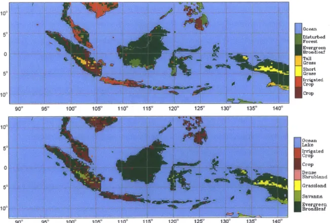
Figure 1-1. Approximate boundary and major islands of the Maritime Continent region... 21 Figure 2-1. Model domain showing the land use classification (top) from GLCC used for
BATS1e and (bottom) from Ramankutty (1999) used for IBIS. ... 31
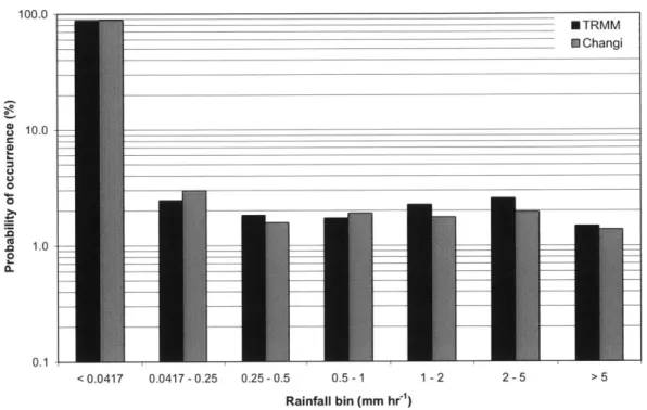
Figure 2-2. Rainfall histogram over Singapore for period 1998-2001: comparison between TRMM (black) and Changi meteorological station (grey). ... 37
Figure 2-3. Average diurnal cycle of rainfall (in mm hr 1) over Singapore for period
1998-2001: comparison between TRMM (solid line) and Changi meteorological station (dashed
lin e )...3 8
Figure 2-4. Rainfall histogram over Maritime Continent for period 1998-2001: comparison between TRMM and the GFC and EMAN simulations.. ... 39
Figure 2-5. Time series of rainfall (in mm hr-') over Singapore for period January - February
1 9 9 8 ... 4 0
Figure 2-6. Diurnal cycle of rainfall from TRMM. Local time for the center of the domain is given at the bottom of each panel. ... 42 Figure 2-7. As for Figure 2-6 but for the GFC simulation. ... 43 Figure 2-8. As for Figure 2-6 but for the EMAN simulation... 44 Figure 2-9. Average diurnal cycle of rainfall (in mm hr 1) over period 1998-2001: comparison
between TRMM, the GFC (red) and EMAN (blue) simulations using ERA40 (solid lines) and NCEP (dashed lines), and the GAS simulation (green). ... 47 Figure 2-10. Rainfall histogram comparing TRMM and the simulations using GFC and EMAN
with both BATS1e and IBIS for period 1998-2001... 50
Figure 2-11. Average diurnal cycle of rainfall (in mm hr-1) over period 1998-2001: comparison between TRMM and the GFC (red) and EMAN (blue) simulations using BATS1e (solid lines) and IBIS (dashed lines) ... 51
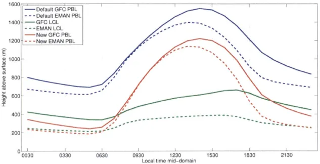
Figure 3-1. Typical daily boundary layer (BL) evolution in a high pressure region over land.. 62 Figure 3-2. Average diurnal cycle of PBL height and elevation of LCL (both in m) over land
cells for period 1998-2001 as simulated by RegCM3-IBIS using the Grell Fritsch-Chappell and Em anuel convection schem es. ... 63
Figure 3-3. Profiles of potential temperature (in 'C) for lowest 3 km of atmosphere from Changi airport radiosonde data, 1 October - 23 November 2010. (a) 8 am LT; (b) 11 am
LT; (c) 2 pm LT; (d) 8 pm LT... 66
Figure 3-4. Profiles of water vapor mixing ratio (in kg/kg) for lowest 3 km of atmosphere from Changi airport radiosonde data, 1 October - 23 November 2010. (a) 8 am LT; (b) 11 am LT; (c) 2 pm LT; (d) 8 pm LT... 68
Figure 3-5. Comparison between (left) geography of Malay Peninsula and (right) model dom ain w ith 30 km grid cells... 69
Figure 3-6. Diurnal PBL height (in m) over or near Singapore, simulated by the (top) Grell Fritsch-Chappell and (bottom) Emanuel convection schemes using either a land (blue) or ocean (green) grid cell to represent Singapore, compared to the PBL height estimated from the Changi soundings (black stars; dotted lines are shown to interpolate between the m easurem ent tim es)... 72
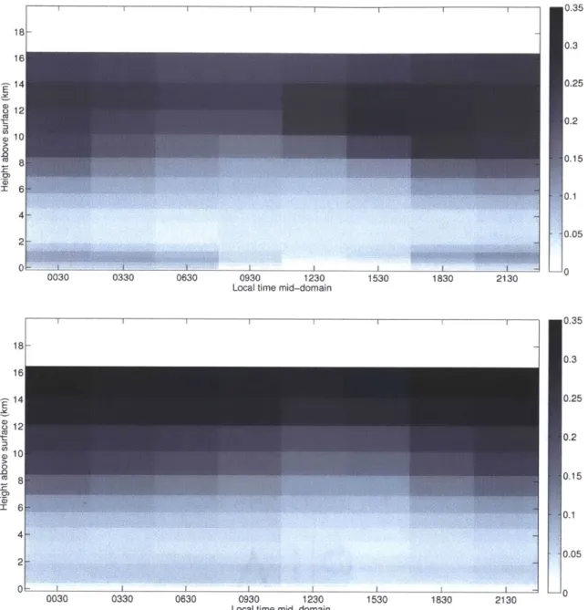
-Figure 3-7. Diurnal cycle of cloud cover averaged over land grid cells within the model domain for the period 1998-2001, using the default RegCM3-IBIS with the Grell (top) and Em anuel (bottom ) convection schem es... 81 Figure 3-8. As for Figure 3-7 but for ocean grid cells. ... 82
Figure 3-9. Average diurnal cycle of original PBL height (blue), new PBL height (red) and elevation of LCL (green) over land cells within the model domain for the period 1998-2001, using RegCM3-IBIS with both the Grell with Fritsch-Chappell closure (GFC, solid
line) and Emanuel (EMAN, dashed line) convection schemes. ... 91
Figure 3-10. Average diurnal cycle of original PBL height (blue), new PBL height (red) and elevation of LCL (green) over ocean cells within the model domain for the period
1998-2001, using RegCM3-IBIS with both the Grell with Fritsch-Chappell closure (GFC, solid line) and Emanuel (EMAN, dashed line) convection schemes... 91
Figure 3-11. Diurnal PBL height (in m) over or near Singapore, simulated by the (top) Grell Fritsch-Chappell and (bottom) Emanuel convection schemes using either a land (blue) or ocean (green) grid cell to represent Singapore, compared to the PBL height estimated from the Changi soundings (black stars; dotted lines are shown to interpolate between the m easurem ent tim es)... 93
Figure 3-12. Diurnal cycle of cloud cover incorporating changes to cloud fraction, averaged for period 1998-2001 using Grell Fritsch-Chappell convection scheme for land (top) and ocean (bottom ) grid cells... 95
Figure 3-13. As for Figure 3-12 but using the Emanuel convection scheme... 96 Figure 3-14. Average low cloud fraction for 1998-2001: simulation minus ISCCP data for (a)
Grell Fritsch-Chappell with default clouds, (b) Emanuel scheme with default clouds, (c) Grell scheme with new PBL cloud cover and (d) Emanuel scheme with new PBL cloud c o v e r.. ... 9 7 Figure 3-15. Diurnal cycle of incoming solar radiation (in W m-2) averaged over land for
period 1998-2001 for SRB observations and simulations using (top) Grell with Fritsch-Chappell and (bottom) Emanuel convection schemes, comparing the default version to the m odified (-M od) version.. ... 102 Figure 3-16. Diurnal cycle of incoming solar radiation (in W m-2) averaged over ocean for
period 1998-2001 for SRB observations and simulations using (top) Grell with Fritsch-Chappell and (bottom) Emanuel convection schemes, comparing the default version to the m odified (-M od) version.. ... 103
Figure 3-17. Diurnal cycle of rainfall (in mm hr1) averaged over land for period 1998-2001, comparing default simulations to the modified version of the model...106 Figure 3-18. Diurnal cycle of rainfall (in mm hr1) averaged over ocean for period 1998-2001, comparing default simulations to the modified version of the model...106 Figure 3-19. Rainfall histogram averaged over land grid cells for period 1998-2001,
comparing TRMM to simulations using Grell with Fritsch-Chappell (GFC) and Emanuel
(EM A N ) convection schem es... 107
Figure 3-20. Rainfall histogram as in Figure 3-19 but averaged over ocean grid cells. ... 107 Figure 4-1. Interactions between various processes in the climate system, showing the key
role played by clouds (Figure 1 in Arakaw a 2004). ... 109
-Figure 4-2. Global annual mean energy fluxes (in W m2
) over the period March 2000 - May 2004 (Figure 1 taken from Trenberth et al. 2009). ... 110
Figure 4-3. Cloud and associated processes for which major uncertainties in formulations exist (Figure 2 from A rakaw a 2004). ... 111
Figure 4-4. Schematic illustration of default calculation of convective cloud fraction within R e g C M 3 .. ... 1 1 8
Figure 4-5. Average low cloud fraction for 1998-2001: simulation minus ISCCP data for (a)
GFC (default model), (b) EMAN (default model), (c) GFC-Mod (as in Chapter 3), (d)
EMAN-Mod (as in Chapter 3), (e) GFC-New (with new FCcoV) and (f) EMAN-New (with new FCcnv).
... 1 2 6
Figure 4-6. Average middle cloud fraction for 1998-2001: simulation minus ISCCP data for (a)
GFC (default model), (b) EMAN (default model), (c) GFC-Mod (as in Chapter 3), (d)
EMAN-Mod (as in Chapter 3), (e) GFC-New (with new FCcnv) and (f) EMAN-New (with new
F C cnv)... ... 1 2 7
Figure 4-7. Average high cloud fraction for 1998-2001: simulation minus ISCCP data for (a)
GFC (default model), (b) EMAN (default model), (c) GFC-Mod (as in Chapter 3), (d)
EMAN-Mod (as in Chapter 3), (e) GFC-New (with new FCcv) and (f) EMAN-New (with new FCcn).. ... 128 Figure 4-8. Average diurnal cycle of cloud cover over land 1998-2001 using Grell
Fritsch-Chappell scheme with new convective cloud fraction and modifications from Chapter 3..
... 130
Figure 4-9. Average diurnal cycle of cloud cover over land 1998-2001 using Emanuel scheme with new convective cloud fraction and modifications from Chapter 3...130 Figure 4-10. Average diurnal cycle of cloud cover over ocean 1998-2001 using Grell
Fritsch-Chappell scheme with new convective cloud fraction and modifications from Chapter 3..
... 1 3 1
Figure 4-11. Average diurnal cycle of cloud cover over ocean 1998-2001 using Emanuel scheme with new convective cloud fraction and modifications from Chapter 3...131 Figure 4-12. Average cloud liquid water (in mg m-3) profile over central Borneo for (a)
CloudSat averaged over period 2006-2011, (b) GFC-Mod, (c) GFC-New, (d) EMAN-Mod, (e) EM AN-New (note the change in x-axis). ... 134 Figure 4-13. Average cloud liquid water (in mg m-3
) profile over western Pacific Ocean for (a) CloudSat averaged over period 2006-2011, (b) GFC-Mod, (c) GFC-New, (d) EMAN-Mod, (e) EM AN-New (note the change in x-axis). ... 136
Figure 4-14. Diurnal cycle of insolation (in W m-2
) averaged over land for period 1998-2001, from SRB observations and simulations using Grell Fritsch-Chappell scheme with modifications from Chapter 3 Mod), and with new convective cloud cover (GFC-N e w ). ... 1 3 8
Figure 4-15. Diurnal cycle of insolation (in W m2
) averaged over land for period 1998-2001,
from SRB observations and simulations using Emanuel scheme with modifications from Chapter 3 (EMAN-Mod), and with new convective cloud cover (EMAN-New).. ... 139
-Figure 4-16. Diurnal cycle of insolation (in W m-2
) averaged over ocean for period 1998-2001, from SRB observations and simulations using Grell Fritsch-Chappell scheme with
modifications from Chapter 3 Mod), and with new convective cloud cover (GFC-N e w ). ... 1 3 9
Figure 4-17. Diurnal cycle of insolation (in W m-2
) averaged over ocean for period 1998-2001, from SRB observations and simulations using Emanuel scheme with modifications from Chapter 3 (EMAN-Mod), and with new convective cloud cover (EMAN-New). ... 140
Figure 4-18. Average diurnal cycle of cloud cover over land 1998-2001 using Emanuel scheme with new convective cloud fraction, modifications from Chapter 3 and CLWT tuned from 1.1 g kg1 to 0.25 g kg '...145 Figure 4-19. Average diurnal cycle of cloud cover over land 1998-2001 using Emanuel
scheme with new convective cloud fraction, modifications from Chapter 3 and CLWT tuned from 1.1 g kg-1 to 0.25 g kg-1. ... 145
Figure 4-20. Average cloud liquid water (in mg m3) profile over (top) central Borneo and (bottom) western Pacific Ocean, simulated using the Emanuel scheme with new
convective cloud fraction, modifications from Chapter 3 and CLWT tuned from 1.1 g kg' to 0 .2 5 g kg ~1. ... 14 6 Figure 5-1. Relationship between fractional cloud cover, FC, and fractional coverage of
ra in fa ll, p ... 1 6 3 Figure 5-2. Average low cloud fraction for 1998-2001: simulation minus ISCCP data for (a)
GFC-Mod, (b) Mod, (c) GFC-New, (d) New, (e) GFC-Auto and (f) EMAN-A u to . ... 1 7 3
Figure 5-3. Average middle cloud fraction for 1998-2001: simulation minus ISCCP data for (a) GFC-Mod, (b) Mod, (c) GFC-New, (d) New, (e) GFC-Auto and (f) EMAN-A u to . ... 1 7 4
Figure 5-4. Average high cloud fraction for 1998-2001: simulation minus ISCCP data for (a) GFC-Mod, (b) Mod, (c) GFC-New, (d) New, (e) GFC-Auto and (f) EMAN-A u to .. ... 1 7 5
Figure 5-5. Average diurnal cycle of cloud cover over land 1998-2001 using Grell Fritsch-Chappell scheme with new autoconversion formulation.. ... 177
Figure 5-6. Average diurnal cycle of cloud cover over land 1998-2001 using Emanuel scheme w ith new autoconversion form ulation...177 Figure 5-7. Average diurnal cycle of cloud cover over ocean 1998-2001 using Grell
Fritsch-Chappell scheme with new autoconversion formulation. ... 178
Figure 5-8. Average diurnal cycle of cloud cover over ocean 1998-2001 using Emanuel
schem e w ith new autoconversion form ulation. ... 178
Figure 5-9. Average cloud liquid water (in mg m3) profile over central Borneo from (a) CloudSat for period 2006-2011, (b) simulation using Grell Fritsch-Chappell scheme with new convective cloud cover for period 1998-2001, (c) as for middle but using Emanuel schem e (note the change in x-axis)...181 Figure 5-10. Average cloud liquid water (in mg m3) profile over western Pacific Ocean from
(a) CloudSat for period 2006-2011, (b) simulation using Grell Fritsch-Chappell scheme with new convective cloud cover for period 1998-2001, (c) as for middle but using Em anuel schem e (note the change in x-axis)...182
-Figure 5-11. Diurnal cycle of incoming solar radiation (in W m-2) averaged over land for period 1998-2001, from SRB observations and simulations using Grell Fritsch-Chappell scheme with modifications from Chapter 3 ('GFC-Mod'), those modifications plus the new convective cloud fraction and CLW from Chapter 4 ('GFC-New') and new
autoconversion formulation combined with all other changes ('GFC-Auto')...184 Figure 5-12. As for Figure 5-11 but with the Emanuel convection scheme...184 Figure 5-13. Diurnal cycle of incoming solar radiation (in W m-2
) averaged over ocean for period 1998-2001, from SRB observations and simulations using Grell Fritsch-Chappell scheme with modifications from Chapter 3 ('GFC-Mod'), those modifications plus the new convective cloud fraction and CLW from Chapter 4 ('GFC-New') and new
autoconversion formulation combined with all other changes ('GFC-Auto')...185 Figure 5-14. As in Figure 5-13 but using the Emanuel convection scheme. ... 185
Figure 5-15. Rainfall histogram, with rainfall intensities in mm hr-1
, averaged over land grid cells for period 1998-2001, comparing TRMM to simulations using Grell with Fritsch-Chappell (GFC) and Emanuel (EMAN) convection schemes with the default version of the model and incorporating all changes made to the PBL, cloud cover and autoconversion in C h a p te rs 3 to 5 . ... 1 9 1
Figure 5-16. As in Figure 5-15 but for ocean grid cells...192 Figure 5-17. Diurnal cycle of rainfall (in mm hr-) averaged over land for period 1998-2001 for
TRMM and the new simulations with all modifications (to PBL region, convective cloud fraction and autoconversion, '-A uto')... 193
Figure 5-18. Diurnal cycle of rainfall (in mm hr') averaged over ocean for period 1998-2001 for TRMM and the new simulations with all modifications (to PBL region, convective cloud fraction and autoconversion, '-Auto'). ... 193
Figure 5-19. Average temperature (in 0C) for period 1998-2001 over land surfaces within the model domain, from (a) CRU TS3.0, (b) lowest atmospheric layer from ERA40, (c) GFC default, (d) EMAN default, (e) GFC-Auto simulation, (f) EMAN-Auto simulation...195 Figure 6-1. Local time (see color bar) of diurnal rainfall peak from TRMM, averaged over
19 9 8 -2 0 0 1 ... 2 10
Figure 6-2. Local time (see color bar) of diurnal rainfall peak averaged over 1998-2001, using Emanuel scheme with the default version of RegCM 3... 211 Figure 6-3. Difference in timing (hours) of diurnal rainfall peak averaged over 1998-2001,
TRMM minus RegCM3-IBIS using Emanuel scheme with the default model.. ... 211
Figure 6-4. Local time (see color bar) of diurnal rainfall peak averaged over 1998-2001, using Emanuel scheme with the new version of RegCM3-IBIS incorporating all modifications presented in Chapters 3 to 5... 212 Figure 6-5. Difference in timing (hours) of diurnal rainfall peak averaged over 1998-2001,
TRMM minus RegCM3-IBIS using Emanuel scheme with the new version of the model incorporating all modifications presented in Chapters 3 to 5.. ... 212 Figure 6-6. Distance to coastline (meters) for each land grid cell within domain...214 Figure 6-7. Topography (meters) used in simulations: the Geological Survey's Global 30 arc
second elevation dataset (GTOPO30), aggregated to 10 arc minutes (United States Geological Survey 1996) and interpolated to the 30 km grid used in simulations...214
14-Figure 6-8. Standard deviation of topography (meters) contained within each 30 km grid cell compared to the GTOPO30 input data interpolated within each grid cell...214 Figure 6-9. Location of sub-regions used in spatial analysis: (A) Malay Peninsula, (B) Highland Borneo, (C) Lowland Borneo, (D) Northern Sumatra, (E) Southern Sumatra. ... 216
Figure 6-10. Diurnal cycle of rainfall (in mm hr') averaged over Malay Peninsula sub-region for period 1998-2001 for TRMM and simulations using Emanuel scheme with default version of the model and version with all modifications (to PBL region, convective cloud fraction and autoconversion)...217 Figure 6-11. Diurnal cycle of rainfall (in mm hr-') averaged over highland Borneo sub-region
for period 1998-2001 for TRMM and simulations using Emanuel scheme with default version of the model and version with all modifications (to PBL region, convective cloud fraction and autoconversion)...217 Figure 6-12. Diurnal cycle of rainfall (in mm hr-) averaged over lowland Borneo sub-region
for period 1998-2001 for TRMM and simulations using Emanuel scheme with default version of the model and version with all modifications (to PBL region, convective cloud fraction and autoconversion)...218 Figure 6-13. Diurnal cycle of rainfall (in mm hr') averaged over northern Sumatra sub-region
for period 1998-2001 for TRMM and simulations using Emanuel scheme with default version of the model and version with all modifications (to PBL region, convective cloud fraction and autoconversion)...218 Figure 6-14. Diurnal cycle of rainfall (in mm hr1) averaged over southern Sumatra sub-region
for period 1998-2001 for TRMM and simulations using Emanuel scheme with default version of the model and version with all modifications (to PBL region, convective cloud fractio n and autoconversion)...219 Figure 6-15. Local time (see color bar) of diurnal rainfall peak averaged over 1998-2001,
using Emanuel scheme with the new version of RegCM3-IBIS incorporating all
modifications presented in Chapters 3 to 5, using 10 km resolution...224 Figure 6-16. Local time (see color bar) of diurnal rainfall peak averaged over 1998-2001,
using Emanuel scheme with the new version of RegCM3-IBIS incorporating all
modifications presented in Chapters 3-5, using 29 vertical layers ... 225
Figure 6-17. Diurnal cycle averaged over the period 1998-2001 of meridional wind (m s') along 1140E through Borneo from simulation using Emanuel scheme with new version of th e m o d e l. ...---... 2 3 0 Figure 6-18. Diurnal cycle averaged over the period 1998-2001 of temperature anomaly ('C,
see color bar) with zonal and vertical winds (m s-1, with vertical wind component
amplified 10 times) along 20S from simulation using Emanuel scheme with new version of
the m o d e l. ...-... - .. ---... 231 Figure 6-19. Diurnal cycle averaged over the period 1998-2001 of longwave radiation (in
W m-2) away from surface (i.e. radiative cooling) from SRB observations.. ... 232
Figure 6-20. Diurnal cycle averaged over the period 1998-2001 of longwave radiation (in W m-2
) away from surface (i.e. radiative cooling) from simulation using Emanuel scheme w ith new version of the m odel.. ... 233
-Figure 6-21. Time-longitude plot along latitude 2'S of diurnal rainfall anomaly, calculated as the rainfall at each time of day minus the daily mean rainfall, averaged over 1998 for the simulation using the new version of the model with the Emanuel scheme...236 Figure 6-22. Time-longitude plot along latitude 20S of diurnal temperature anomaly (in C),
calculated as the temperature at each time of day minus the daily mean temperature, averaged over 1998 for the simulation using the new version of the model with the Em anuel schem e.. ... 237
Figure 6-23. Schematic of rainfall processes over Borneo at approximately 1000-1200 LT..241 Figure 6-24. Schematic of rainfall processes over Borneo at approximately 1600 LT...241 Figure 6-25. Schematic of rainfall processes over Borneo at approximately 2000-2200 LT. 242 Figure 6-26. Schematic of rainfall processes over Borneo at approximately 0000-0200 LT. 242 Figure 7-1. Schematic showing the typical circulation and temperature patterns over the
Pacific Ocean under (left) average and (right) El Niho conditions during the northern winter. El Nino episodes feature reduced easterly winds across the Pacific in the lower atmosphere and reduced westerly winds in the upper atmosphere. ... 244
Figure 7-2. Average cloud fraction over 1983-2001: EMAN-Def simulation minus ISCCP data for (a) low, (c) middle and (e) high clouds, and EMAN-New simulation minus ISCCP data
for (b) low , (d) m iddle and (f) high clouds... 248
Figure 7-3. Average rainfall (in mm day-) for period 1983-2001, from (a) CRU TS3.0, (b) GPCP V2.2, (c) EMAN-Def (default) simulation, (d) EMAN-New simulation (incorporating all
m odifications presented in Chapters 3 to 5)... 251 Figure 7-4. Average temperature (in 0
C) for period 1983-2001 over land surfaces within the
model domain, from (a) CRU TS3.0, (b) lowest atmospheric layer from ERA40, (c) EMAN-Def (default) simulation, (d) EMAN-New simulation (incorporating all modifications presented in Chapters 3 to 5)... 253
Figure 7-5. 3-month moving average of rainfall over land for period 1983-2001, comparing
GPCP (black), TRMM (blue; only for period 1998-2001), default version of RegCM3-IBIS
using Emanuel scheme (green) and improved version of the model (red). ... 262
Figure 7-6. 3-month moving average of rainfall over land for period 1983-2001, comparing
GPCP (black), TRMM (blue; only for period 1998-2001), default version of RegCM3-IBIS
using Emanuel scheme (green) and improved version of the model (red). ... 264
Figure 7-7. Rainfall (mm day-) over land for period 1983-2001, showing the difference between the 3-month moving average and the mean rainfall for GPCP (black), TRMM (blue; only for period 1998-2001), default version of RegCM3-IBIS using Emanuel scheme (green) and im proved version of the m odel (red). ... 264
Figure 7-8. 3-month moving average of rainfall over ocean for period 1983-2001, comparing
GPCP (black), TRMM (blue; only for period 1998-2001), default version of RegCM3-IBIS
using Emanuel scheme (green) and improved version of the model (red). ... 264
Figure 7-9. 3-month moving average of rainfall over ocean for period 1983-2001, comparing
GPCP (black), TRMM (blue; only for period 1998-2001), default version of RegCM3-IBIS
using Emanuel scheme (green) and improved version of the model (red).. ... 266
-Figure 7-10. Rainfall (mm day') over ocean for period 1983-2001, showing the difference between the 3-month moving average and the mean rainfall for GPCP (black), TRMM (blue; only for period 1998-2001), default version of RegCM3-IBIS using Emanuel scheme (green) and im proved version of the m odel (red). ... 266
Figure 7-11. Average seasonal rainfall (mm day-) over land, comparing GPCP (black), default (green) and improved (red) versions of the model averaged for the period 1983-2001, and TRM M (black) averaged over the period 1998-2001...267 Figure 7-12. Average seasonal rainfall (mm day-) over ocean, comparing GPCP (black),
default (green) and improved (red) versions of the model averaged for the period 1983-2001, and TRMM (black) averaged over the period 1998-2001...268 Figure A-1. Left: The relationship between cloud water (in mm) and precipitation water (in
mm) in UMORA. Middle: The same relationship for GPROF, where the black line indicates the UMORA relationship. Right: The relationship between surface rain rate (in mm hr-) and colum nar average rain rate (in mm hr') in GPROF...286 Figure A-2. Retrieved partition for cloud and rain liquid water path (LWP) (in kg m-2) during the w hole observation period (Class 2)...287
-List of Tables
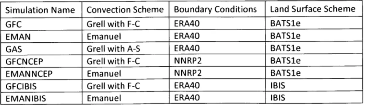
Table 2-1. Characteristics of simulations used in the assessment... 33
Table 2-2. Average daily rainfall over land and ocean over period 1998-2001 for each
simulation presented in this assessment, with TRMM values shown for comparison...46 Table 2-3. Simulated average daily land surface energy fluxes and evapotranspiration
com ponents over period 1998-2001... 52
Table 2-4. Measured values of ET, interception loss and transpiration from field studies...54 Table 3-1. PBL height (in m) over Changi airport estimated qualitatively from radiosonde data using depth of constant potential temperature (theta) and water vapor mixing ratio. ... 65 Table 3-2. PBL height (m) over Singapore estimated from radiosonde data using condition 1
o f H effte r (19 8 0)... 6 8
Table 3-3. Mean wind speed (in m s') and direction (in deg) measured by Changi Airport so u n d in g s...7 0
Table 3-4. PBL height (in m) comparison between Changi sounding estimate and values simulated using new PBL modifications, over land and ocean model grid cells...92 Table 3-5. Average daily surface radiative and turbulent heat fluxes (all in W m2
) over period
1998-2001 for simulations using the default and modified model. ... 98
Table 3-6. Average daily rainfall (in mm day') over land and ocean over period 1998-2001 for simulations with default and modified versions of the model. ... 104
Table 4-1. Method for treatment of convective cloud fraction in selected large-scale climate m o d e ls. ... 1 1 7
Table 4-2. Observations of cloud liquid water content used to calculate new convective cloud fra ctio n . ... 1 2 2
Table 4-3. Average daily surface radiative and turbulent heat fluxes over period 1998-2001 for SRB (radiative fluxes) and field studies (LH and SH) ('Obs.') and simulations using the
modifications from Chapter 3 ('-Mod') and new convective cloud fraction ('-New')...142 Table 4-4. Total, convective and large-scale rainfall averaged over 1998-2001 for land and
ocean from TRMM, modified simulations (from Chapter 3, 'mod') and simulations with new convective cloud cover and CLW ('new')...143 Table 4-5. Radiative and turbulent fluxes averaged over 1998-2001 from SRB (radiative
fluxes) and field studies (LH and SH) ('Obs.') compared to simulations using the Emanuel scheme, modified (from Chapter 3, 'mod'), with new convective cloud cover and Chapter
3 m odifications ('new '), and w ith CLW T tuned...147
Table 4-6. Total, convective and large-scale rainfall averaged over 1998-2001 for land and ocean from TRMM ('Observations') and simulations using the Emanuel scheme, modified
(from Chapter 3, 'mod'), with new convective cloud cover and Chapter 3 modifications ('new '), and w ith CLW T tuned. ... 147 Table 5-1. Autoconversion functions in selected climate models. ... 160
Table 5-2. Observations used to constrain new autoconversion function...167 Table 5-3. Average daily surface radiative and turbulent heat fluxes over period 1998-2001
for SRB (radiative) and field studies (LH and SH) ('Obs.'), compared to simulations using the modifications from Chapter 3 ('-Mod'), those modifications plus the new convective
-18-cloud fraction and CLW ('-New'), and simulations with the new autoconversion
form ulation com bined with all other changes ('-Auto'). ... 187
Table 5-4. Total, convective and large-scale rainfall averaged over 1998-2001 for land and ocean from TRMM ('Observations'), modified simulations (from Chapter 3, '-Mod'), simulations with new convective cloud fraction and CLW ('-New') and simulations with
new autoconversion form ulation ('-Auto'). ... 189
Table 5-5. Near-surface temperature (T, in 0C), water vapor mixing ratio (Q, in g kg-') and
relative humidity (RH, in %) averaged for the period 1998-2001 over land and ocean surfaces w ithin the m odel dom ain...198 Table 6-1. Mean characteristics of locations within model domain exhibiting similar error in
timing of diurnal rainfall peak with respect to TRMM, comparing the Emanuel scheme with the default version of RegCM3-IBIS to the new version incorporating all
m odifications presented in Chapters 3 to 5...215
Table 6-2. Total, convective and large-scale rainfall averaged over 1998-2001 for each sub-region shown in Figure 6-11, comparing the Emanuel scheme with the default version of RegCM3-IBIS to the new version incorporating all modifications presented in Chapters 3 to 5 ... 2 2 1
Table 6-3. Average daily surface radiative fluxes over period 1998-2001 for SRB
('Observations') and for each sub-region shown in Figure 6-11, comparing the Emanuel scheme with the default version of RegCM3-IBIS to the new version incorporating all m odifications presented in Chapters 3 to 5...222 Table 6-4. Average daily surface radiative fluxes over period 1998-2001 for SRB
('Observations') and for simulations using the Emanuel scheme with the new version of RegCM3-IBIS incorporating all modifications presented in Chapters 3 to 5, for different vertical and horizontal resolutions...223 Table 6-5. Total, convective and large-scale rainfall averaged over 1998-2001 for land and
ocean from TRMM ('Observations') and for simulations using the Emanuel scheme with the new version of RegCM3-IBIS incorporating all modifications presented in Chapters 3 to 5, for different vertical and horizontal resolutions...223 Table 7-1. Average daily surface radiative and turbulent heat fluxes over 19-year period
1983-2001 and 4-year period 1998-2001, comparing SRB (radiative fluxes) and field
studies (LH and SH) ('Obs.') to the Emanuel scheme with the default version of RegCM3-IBIS (EMAN-Def) and the new version incorporating all modifications presented in
Chapters 3 to 5 (EM A N -N ew ). ... 250
Table 7-2. Total, convective and large-scale rainfall averaged over 1983-2001 for land and ocean for the EMAN-Def and EMAN-New simulations...252 Table 7-3. Warm (red) and cold (blue) episodes over the eastern Pacific Ocean based on a
threshold of +/- 0.5 0C for the Oceanic Nino Index (ONI), based on centered 30-year base
periods updated every 5 years... 255
Table 7-4. Average daily surface radiative fluxes for El Nino and La Niia episodes from SRB ('Obs.') and the EMAN-Def and EMAN-New simulations...258 Table 7-5. Total, convective and large-scale rainfall (all in mm day-) for El Nino and La Nina
periods over land and ocean for the EMAN-Def and EMAN-New simulations...260
-20-Chapter 1: Introduction
History teaches us that simulation without understanding can be perilous, and is in any case intellectually empty.
- Kerry Emanuel
1.1 Motivation
The Maritime Continent region is home to approximately 375 million people. It is the portion of Southeast Asia comprising Malaysia, Indonesia, Brunei Darussalam, Singapore, East
Timor and the Philippines, approximately bounded by 900E - 1400E and 100S - 10ON (Figure 1-1). It contains thousands of islands, ranging in size from tens to thousands of kilometers,
with steep topographic gradients: the two highest peaks in the region are 4884 m in the Indonesian province of Irian Jaya (western New Guinea) and 4100 m in the Malaysian
province of Sabah (northeastern Borneo). The islands are interspersed by segments of ocean with depths varying from as little as 50 m in parts of the South China Sea to as much as
5000 m in the Pacific and Indian Ocean basins. Few regions of the world contain such
dramatic geographic variability in relatively small spatial scales as the Maritime Continent.
10*
0
90* 95* 1000 105* 11 115 120* 125* 13 135 140
Figure 1-1. Approximate boundary and major islands of the Maritime Continent region. The color gradient indicates relative topographic gradients over the islands.
Rainfall is generally very high over this region, with annual precipitation totals of
about 2700 mm. The Maritime Continent is located at the western edge of the oceanic
-21-'warm pool', where sea surface temperatures are approximately 300C year round, and the rising branch of the Pacific Ocean's Walker circulation. During the months of December-February, the region also lies within the Intertropical Convergence Zone (ITCZ) and it is influenced by both the South Asian and East Asian monsoons, associated with seasonal movement of the ITCZ. Therefore the large-scale conditions influencing this region are generally conducive to strong convection.
It has long been known that convective storms over the tropics are responsible for significant inputs of heat and moisture to the upper troposphere, due to large releases of
latent heat and the production of dense clouds that shield from radiative cooling (Ramage
1968). Given the importance of convective processes in the Maritime Continent to global
rainfall and circulation processes, accurate simulation of the climate of this region is critical for simulations of both regional and global circulations (Neale and Slingo 2003).
However, current predictions of climate change over the Maritime Continent still contain a high degree of uncertainty. The Fourth Assessment Report of the
Intergovernmental Panel on Climate Change ('the IPCC report') noted that, although the performance of regional climate models has improved significantly over many parts of the world, simulations over the Southeast Asian region still demonstrate significant variation in projected impacts from climate change (Christensen et al. 2007), indicating that the
mechanisms driving rainfall in this region are still not adequately understood or represented in climate models. The IPCC report also noted that local impacts of climate change are likely to vary significantly within Southeast Asia due to the region's complex topography and oceanic influences (Christensen et al. 2007).
Southeast Asia has been identified as a region highly vulnerable to climate variability, due to its long coastlines, high concentration of people and economic activity in coastal areas, heavy reliance on agriculture and natural resources, and variable adaptive capacity (Nitivattananon et al. 2013). Particular sources of projected risk are increases in diarrhoeal
disease, associated with floods and droughts, and epidemics of malaria, dengue and other vector-borne diseases (Cruz et al. 2007). These human health risks are all strongly
dependent on local and regional climatic and hydrologic conditions. We therefore have a
-critical need to improve our ability to simulate processes related to rainfall over the Maritime Continent.
1.2 Background
The diurnal cycle of rainfall and temperature is one of the strongest modes of variability in the climate of the Maritime Continent (Yang and Slingo 2001, Kitoh and
Arakawa 2005). Specific studies undertaken to better understand the diurnal cycle over the Maritime Continent include the Island Thunderstorm Experiment (ITEX; e.g. Keenan et al.
1989, Simpson et al. 1992), the Maritime Continent Thunderstorm Experiment (MCTEX;
Keenan et al. 2000), the Tropical Oceans-Global Atmosphere Coupled Ocean-Atmosphere Response Experiment (TOGA-COARE; e.g. Liberti et al. 2001), and the Tropical Warm Pool-International Cloud Experiment (TWP-ICE; May et al. 2008). These studies used detailed site-specific data obtained primarily from ground-based radar and meteorological stations or ocean buoys. In more recent years, satellite-based observations have provided a more spatially coherent picture of the diurnal rainfall cycle over the region (e.g. Hall and Vonder Haar 1999, Sorooshian et al. 2002, Nesbitt and Zipser 2003, Mori et al. 2004, Janowiak et al.
2005, Ichikawa and Yasunari 2006, Yang and Smith 2006). In particular, the diurnal cycles of
convection and rainfall propagation have been well described for the islands of Sumatra (Mori et al. 2004, Sakurai et al. 2005, Wu et al. 2009b), Borneo (Ichikawa and Yasunari 2006, Hara et al. 2009, Wu et al. 2009a), New Guinea (Zhou and Wang 2006, Ichikawa and Yasunari
2008) and the Malay Peninsula (Joseph et al. 2008).
The dominant diurnal signal over the Maritime Continent has been attributed to local insolation-driven instability and circulations initiated by differential responses to insolation (e.g. Saito et al. 2001, Yang and Slingo 2001, Slingo et al. 2003, Qian 2008). Land-sea breeze circulations are the most well-known of these and have been studied extensively (e.g.
Neumann and Mahrer 1974, Baker et al. 2001, Zhou and Wang 2006). The smaller heat capacity of the land surface compared to the ocean causes differential radiative heating
during the daytime, creating a much larger diurnal temperature variation over land than over ocean. The comparatively lower pressure over land produces a sea breeze in the late morning to early afternoon, which initiates convection over land-ocean boundaries. Similar
-circulations are created by differential heating between mountain and lowland areas. Convective cells are observed to aggregate into mesoscale convective systems (MCSs) in areas of strong convergence, particularly over mountains, leading to prolonged rainfall overnight. Over flat areas, convection can also be initiated or enhanced by the collision of two sea breezes, as shown by Joseph et al. (2008) over the southern Malay Peninsula and by Qian (2008) over Java. These circulations and other diurnal processes will be discussed further later in this thesis.
Generally, more daily total rainfall falls over land than over ocean, because the larger diurnal variations in land surface temperature create greater low-level instability (Neale and Slingo 2003). But the timing and magnitude of the diurnal rainfall cycle varies significantly by the relative size of an island or body of water and the proximity to a coastline. Mountainous areas of the larger islands are observed to produce more rainfall than the flat coastal areas; coastal ocean areas generally exhibit significantly higher diurnal variations in rainfall than the open ocean. It is thought that much of the variability observed over the oceans within the Maritime Continent may be related to MCSs that start over land then move away over the oceans with the land breeze (Liberti et al. 2001, Saito et al. 2001, Mori et al. 2004, Ichikawa and Yasunari 2008). Gravity waves initiated by land-based convection are also thought to be a mechanism for propagation of rainfall over coastal oceans (Yang and Slingo 2001, Mori et al. 2004). Zhou and Wang (2006) showed that offshore propagation of rainfall near New Guinea results from a combination of land breezes and gravity waves forced by deep convection over the steep mountains of the island. This propagation of convection will also be discussed further later in this thesis.
Various studies have shown that global climate models (also general circulation models; GCMs) struggle to accurately reproduce the observed climate over the Maritime Continent region, with land areas having either a wet bias (e.g. Dai and Trenberth 2004, coupled model in Martin et al. 2006) or a dry bias (e.g. Yang and Slingo 2001, atmosphere-only model in Martin et al. 2006), usually accompanied by underestimation of rainfall over
the oceans (e.g. Collier and Bowman 2004, Neale and Slingo 2003). It has been suggested that the source of these errors includes poor representation of the diurnal cycle of
-24-convection over land and the complex circulation patterns generated by land-sea contrasts (Martin et al. 2006), in part because the coarse resolution of GCMs is insufficient to
physically represent the processes that occur over the subgrid-scale islands within the Maritime Continent (Hahmann and Dickinson 2001, Neale and Slingo 2003).
Failure to accurately simulate rainfall processes has flow-on effects to simulation of the land surface hydrology. It was suggested by Dai and Trenberth (2004) that GCMs will also fail to capture nonlinear processes impacting the diurnal cycle of land surface hydrology, such as the different partitioning of rainfall into evaporation and runoff that occurs when
rainfall is simulated during the daytime rather than night-time. Indeed, simulation of the diurnal rainfall cycle is notoriously problematic for GCMs, with the most common error being the early occurrence of daily peak precipitation around midday in simulations, about 4-6
hours ahead of observations (e.g. Yang and Slingo 2001, Collier and Bowman 2004, Dai and Trenberth 2004). Therefore it seems apparent that accurate representation of precipitation
over the Maritime Continent can only be achieved by a model that can adequately capture processes occurring at scales of 10-100 km.
However, relatively few studies using regional climate models (RCMs), typically run at resolutions of tens of kilometers, have been conducted over the Maritime Continent. The previous studies suggest that systemic problems exist with regard to the simulation of diurnal, small-scale processes within large-scale climate models.
Francisco et al. (2006) applied Regional Climate Model (RegCM, maintained at the International Center for Theoretical Physics) to simulation of monsoonal rainfall over the Philippines. In general, the model could reproduce the observed monsoonal rainfall patterns well, but its performance depended strongly on the choice of forcing boundary conditions and the ocean flux scheme (Francisco et a/. 2006). As a result, different combinations of forcing fields and flux parameterizations provided good simulation of rainfall and made it difficult to determine which model user choices were the most appropriate.
Wang et al. (2007) used Regional Climate Model (developed at the International Pacific Research Center) to simulate the diurnal cycle over the Maritime Continent. Those authors found that the model could reasonably reproduce the diurnal cycle, with afternoon
-rainfall maxima over land areas and night-time maxima over ocean areas, but with a time shift that was about 2-4 hours too early compared with satellite observations. The authors found some improvement in model performance by changing the value of the convective entrainment / detrainment rate (Wang et al. 2007).
Joseph et al. (2008) used the Coupled Ocean / Atmosphere Mesoscale Prediction System (COAMPS) with nested domains to simulate rainfall and flow fields around the Malay Peninsula on 23 April 2002. The model reproduced observations reasonably well, but with a cold bias over land during the daytime and a rainfall peak too early in the day by about an
hour (Joseph et al. 2008).
Qian (2008) used Regional Climate Model Version 3 coupled to Biosphere
Atmosphere Transfer Scheme Version le to simulate the diurnal rainfall cycle over the island of Java, Indonesia. The model system was able to reproduce the diurnal cycle reasonably well, but again the timing of the rainfall peak was too early in the day (Qian 2008).
Previous studies have shown consistent error in simulations by GCMs and RCMs over the Maritime Continent region. However, the literature is scarce on detail as to the precise nature of these errors and how they might be addressed. It is often said that models are the laboratories of climate scientists: tools that provide better understanding of the myriad of physical processes occurring in this extremely large and complex system. But the use of these tools relies on a solid grasp of both the processes we wish the model to simulate and the design and intention of the model itself. The latter point has become increasingly
important as GCMs and RCMs have grown in size and complexity, incorporating the work of multitudes of scientists spanning a wide variety of specialist fields. To improve our
simulations of the existing climate and our projections of future climate variability, we need to better understand both the natural world and our tools for studying it.
1.3 Thesis Structure
This thesis investigates diurnal processes related to convection over the Maritime Continent region. It aims to better understand why large-scale climate models fail to capture these processes and how more physically-realistic simulations might be achieved. In
-26-particular, this work is concerned with the convective-radiative feedback and the role of cumulus clouds in mediating the diurnal cycle of rainfall.
Chapter 2 provides a description of the coupled model system used in this work and assesses its performance with regard to simulation of the existing climate of the Maritime Continent region, particularly rainfall.
Chapter 3 more closely investigates simulation of the near surface environment. It describes modifications made to improve simulation of the planetary boundary layer height, non-convective clouds within the planetary boundary layer and surface turbulent heat fluxes. The simulated boundary layer height over Singapore is compared to a dataset obtained specifically for this study.
Chapter 4 describes a new method for parameterizing convective cloud fraction, which relies on observed climatologies of cloud water content and accounts for subgrid variability in cloud cover. It is shown that the new method provides the necessary convective-radiative feedback that was previously absent in the model.
Chapter 5 describes a new method for parameterizing the conversion of cloud droplets into rainfall within large-scale climate models. The new method is constrained by observations of cloud droplets, distributions of cloud water content, and climatological rainfall intensity. It is shown that this method can significantly improve the simulation of
both the diurnal-scale processes and mean climate of the Maritime Continent. Chapter 6 explores the spatial variability of the diurnal rainfall cycle over the Maritime Continent. Behavior over the larger islands is explored in more detail with a view to isolating the specific processes that cannot be captured with a large-scale climate model.
Chapter 7 explores the influence of El Nino and La Niia events on convective rainfall and the diurnal cycle at both the regional and sub-regional scale. It is shown that the improved version of the model capably reproduces the interannual variability observed across the region.
Chapter 8 summarizes the conclusions that can be drawn from this work and provides recommendations for future studies.
Additional information is provided in an appendix for the interested reader.
-28-Chapter 2: Model Description and
Assessment
The work presented in this thesis investigates the diurnal cycle of convective processes over the Maritime Continent using the Regional Climate Model Version 3 (RegCM3) coupled to the land surface models Biosphere Atmosphere Transfer Scheme Version le (BATS1e) and Integrated Biosphere Simulator (IBIS). The first task when
commencing work with a climate model, before it can be used as an experimental tool, is to evaluate its ability to reproduce observations of the existing climate. To that end, this chapter provides a description of the coupled model system and evaluates its performance over the Maritime Continent, with particular attention paid to the simulation of rainfall.
RegCM3-BATS1e has previously shown good results in simulating the large-scale rainfall patterns caused by the monsoon systems over tropical West Africa, South America and South Asia (Pal et al. 2007). Therefore it is also expected to show good performance in simulating the large-scale dynamics over the Maritime Continent. RegCM3-BATS1e has been used over Java (Qian 2008) and an earlier version has been used over the Philippines
(Francisco et al. 2006), but a detailed investigation of the model's performance over the Maritime Continent as a whole and with respect to diurnal and spatial variability in rainfall has yet to be undertaken. In addition, the RegCM3-IBIS model system is untested over the Maritime Continent.
2.1 Model Description
Regional Climate Model (RegCM) was originally developed at the National Center for Atmospheric Research (NCAR) and is now maintained by the International Center for
Theoretical Physics (ICTP). It is a three-dimensional, hydrostatic, compressible, primitive equation, a-coordinate regional climate model. The dynamical core of RegCM3 is based on the hydrostatic version of the Pennsylvania State University / NCAR Mesoscale Model
Version 5 (MM5; Grell et al. 1994) and employs NCAR's Community Climate Model Version 3
(CCM3) atmospheric radiative transfer scheme (described in Kiehl et al. 1996). Planetary