Controller reduction by H[infinity]-balanced truncation

LIDS-P-2025

Controller Reduction by 7-4-Balanced

Truncation

Denis Mustafa*

Keith Glover

Laboratory for Information

Department of Engineering

and Decision Systems

Cambridge University

Massachusetts Institute of

Cambridge CB2 1PZ, UK

Technology

Cambridge MA 02139, USA

(0223) 332711

(617) 253-2156

February 5. 1990

Revised July 25, 1990

To appear in the IEEE Transactions on Automatic Control

Abstract

7-F,0-balanced truncation may be used to obtain reduced-order plants or

con-trollers. The plant (possibly unstable) is compensated using a particular robustly stabilizing controller. The two Riccati equations involved are then used to define a set of closed-loop input-output invariants called the 71, -characteristic values. That0

part of the plant or controller corresponding to 'small' %7'/-characteristic values is discarded to give a reduced-order plant or controller. By exploiting an intimate connection with coprime factorization, a simple a priori test is derived for the abil-ity of such a reduced-order controller to stabilize the full-order plant. Furthermore, the performance of the resulting closed-loop may also be bounded a priori i.e., in terms of the prespecified level of robustness and the discarded 7-/,-characteristic

values.

1

Introduction

Controllers of low complexity are often desirable in practice. Unfortunately, modern controller design techniques frequently lead to high complexity controllers. So there is

'Financial support by the Commonwealth Fund under its Harkness Fellowships program, and by

a real need for reliable model reduction methods which allow a low order controller to be extracted from a high order controller without incurring too much error.

One way of obtaining a low order controller is to work with a low order plant. For example, one well-established way of obtaining a low order plant is the so-called

balanced truncation method initiated in [24]. The state-space description of a stable

system is transformed to balanced coordinates, where the observability and control-lability Gramians are equal and diagonal ('balanced'). The diagonal elements of the balanced Gramian in fact form a set of closed-loop input-output invariants (the Hankel singular values) which quantify the contribution of each state to the input-output map of the system. States contributing only weakly to the input-output map are deleted. The method has some appealing properties: it generically leads to a stable reduced-order model and an error bound exists in terms of the truncated Hankel singular values (see [8, 6J and Lemma 2.3).

Intuitively, however, there are objections to reducing the order of the plant without regard for the controller to be designed for that reduced-order plant. As pointed out in [1], approximation early in a design process may lead to the undesirable propaga-tion of errors as the design progresses. Furthermore, as argued in [6, 33], satisfactory approximation of the plant should take account of the presence of the controller. Open-loop balanced truncation suffers from these criticisms, and if the plant happens to be unstable, compensation is needed anyway. Closed-loop model reduction, where there is some compatibility between the model reduction and the control strategy, would not suffer from these objections.

One closed-loop model reduction procedure was introduced in [161. The open-loop system (which may be unstable) is first compensated with a standard Linear Quadratic Gaussian controller (the so-called Normalized LQG Controller). Two algebraic Riccati equations are needed-one for filtering and one for control. Balancing the solutions to these two Riccati equations, so that they are equal and diagonal, exposes the difficulty of filtering and controlling each state. To be exact, the diagonal elements .i of the solution to the 'LQG-balanced' Riccati equations form a set of closed-loop input-output invariants, known as the LQG-characteristic values. States corresponding to small /i are easy to filter and control in an LQG sense; these states may be discarded to give a reduced-order plant or reduced-order LQG-controller.

More recently there has been much research in the design of 7',,O controllers, which are robust to system uncertainty (see [7] for background). In [25], it was shown how LQG-balancing ideas can be carried over to the corresponding 74,, case. That is, first compensate a plant with a standard 7H,o controller (called the Normalized 7',t

controller), then balance the solutions to the Riccati equations to define a set of

input-output invariants (called the -,oo-characteristic values, vi). States corresponding to small vi are easy to filter and control in an 3,o sense: these states may be discarded to give a reduced-order plant or a reduced-order HOO controller. Only a brief analysis of this 1oo-balanced truncation method of model reduction was given in [25]. Two important questions in particular were not answered:

. How 'small' do the truncated 7H,-characteristic values have to be to guarantee that a reduced-order controller stabilizes the full-order plant?

* What is the degradation in performance caused by using a reduced-order controller in place of the full-order controller?

As well as providing a complete description of the 7ioo-balancing approach and of

7-o-characteristic values, we will also answer the above two questions.

A different approach to obtaining reduced-order LQG or 7/,' controllers may be found in [15] and f3], respectively. (See also [13] for an LQG/'H,o plant reduction problem to which similar methods are applied.) There a fixed (reduced-order) structure for the controller is assumed and optimization theory is applied to derive four coupled matrix equations which the controller state-space matrices must satisfy (two Riccati equations and two Lyapunov equations in the LQG case, four Riccati equations in the

7'tm case). Our approach, in contrast, whilst not known to be optimal, only requires the

pair of decoupled Riccati equations needed for the full-order Normalized 14' Controller. The layout of this paper is as follows. Sections 2 and 3 are preliminary sections, included for completeness: Section 2 summarizes the balanced truncation method of [24] whereas Section 3 summarises the LQG-balancing method of [16]. Some readers may already be very familiar with the material in Sections 2 and 3. In that case they may wish to skip directly to Section 4 which begins the treatment of Ho-balanced truncation with a discussion of XO-balancing and '7,o-characteristic values as introduced in [25]. Section 5 contains the main results of the paper. There the tCO-balanced truncation method is analysed in detail. The analysis hinges on exploiting a close relationship with coprime factorization. Stabilizing and performance properties of the reduced-order controllers are derived, and a numerical example is provided to illustrate the utility of the results. Conclusions are given in Section 6, and Appendices A-C contain proofs of the main results.

Notation All systems are taken to be linear, multivariable and time-invariant, with real-rational transfer function matrices. In general, capital letters are used for matrices and lower case letters are used for vectors. Often we will not distinguish between a (continuous) time domain signal w(t) and the Laplace domain signal w(s); the context will make it clear which is intended. A (proper) transfer function matrix is represented in terms of state-space data by

or

b

,C:= D + C(s-l - )-iB,

or by (A, B, C, D), where A. B, C and D are real matrices of appropriate dimensions.

If D = 0, then the system is strictly proper and we write (A,B,C). The matrix A is asymptotically stable if and only if each of the eigenvalues of A has a strictly negative real part. The symbol IR denotes the real numbers; the prefix R denotes 'real-rational'. We will need the usual Hardy space 7 7_{i{o consisting of real-rational} transfer matrices bounded on the imaginary axis with analytic continuation into the right half plane. (See [7] for further details). If X(s) E 7ZR-, then the 7-₀o-norm of X is defined by ]IXKl[ := sup{\ma,,(X*(jw )X(jw))}, where X*(.s) := XT(-s). If .(s) := (A,B, C. D) then X E 7Z7oo if .A is asymptotically stable. Suppose M = MT

solves the algebraic Riccati equation

ATM + MA- MRM + Q = 0

where R = RT and Q = QT. Then M is said to be the stabilizing solution if A - RM is asymptotically stable. Note that if a stabilizing solution exists, it is unique (see [17,

Lemma 3.4.1]).

2

Balanced Truncation

For completeness and later reference, in this section we give a brief summary of the balanced truncation method of model reduction proposed in [24].

Consider an n state, minimal and asymptotically stable system G = (A, B, C). Its controllability Gramian P = pT E IRnXn is given by the unique positive definite solution to the Lyapunov equation

PAT + AP + BBT = 0. (1)

Its observability Gramian Q = QT E IR"Xn is given by the unique positive definite solution to the Lyapunov equation

QA + ATQ + CTC = 0. (2)

Under a nonsingular state transformation S, (A, B, C) s (SAS-'.SB, C'S-), so Q

9

S-TQS-1 and P s SPST. Hence QP s S-TQpST. Since QP and S-TQpST are

similar matrices, the eigenvalues of QP are similarity invariants. These invariants are the squares of the Hankel singular values of the system G (see e.g., [8]); a formal definition and some basic properties are given next. It is well-known that the largest singular value is the Hankel norm of G.

Proposition 2.1 (Balancing and Hankel singular values [24, 8])

Let the system G = (A, B, C) be minimal and asymptotically stable with n states, and with (positive definite) controllability Gramian P solving (1) and (positive definite) observability Gramian Q solving (2). Then the eigenvalues of QP are real. strictly positive similarity invariants, as are their positive square roots which are called the

Hankel singular values of G. Let arl > a2 > ... > a2 > 0 denote the n eigenvalues of QP arranged in decreasing order, then there exists a similarity transformation which

transforms both Q and P to the form E := diag(-al,a2,... on). The system is then,

said to be in balanced coordinates with balanced Gramian E.

For a given system a balancing transformation can be calculated using the method in [8, Section 4].

In [24] it was argued that, in a balanced realization. the ith Hankel singular value quantifies how observable and controllable the ith state is. Those states with 'small' Hankel singular values may be truncated to leave a reduced-order plant, with only a 'small' error. The details are given next.

Procedure 2.2 (Reduced-order plant by balanced truncation [24])

Let G = (A,B, C) be minimal and asymptotically stable with n states, and in balanced coordinates with Hankel singular values orl - o2 > ... > o > 0. That

is. := cliag(a<,cr2,...,cr, ) = P = Q is the unique positive definite solution of both (1) and (2). Pick k < n and partition E accordingly into

= diag(l,... ) and diagk+l, ,) Parttion .4, and C where 2d = diag(ol,... k) and 22 = diag(ok+l*..on). Partition A, B and C conformably with the partitioning of 2:

A2

1

BA1[B1

= A, 1A 2 B2 an] d C [ C C2 ] (3)

A k-state reduced-order plant is then G, = (All, B1, C1).

Lemma 2.3 Let G be asymptotically stable and minimal with n states. Let k < n and G, be a k-state reduced-order plant obtained by balanced truncation (Procedure 2.2).

Then

(i) [32] G, is in balanced coordinates with balanced Gramian t1. (ii) [32] IfO k > crk+l then G, is asymptotically stable and minimal.

(iii) [8, 6] IlG- GIlo

<-

2 trace[Z2].

Note carefully that item (iii) above gives an error. bound in terms of the truncated Hankel singular values. The existence of such an a priori error bound is one of the attractions of model reduction by balanced truncation.

3

LQG-Balancing and LQG-Characteristic Values

Although balanced truncation has some attractive features it is an open-loop model reduction procedure; no account is taken of the presence of a controller, which may not be realistic (especially if the plant is unstable). Instead, consider a closed-loop procedure where the plant is first stabilized with a standard ('normalized') controller, and then balanced truncation ideas are applied to the closed-loop system. For example, one might connect the plant G to a standard LQG controller and balance that configu-ration, or one might do the same with a standard lHo controller. The former idea was introduced in [16] and is described in this section; the latter idea was introduced in [25] and is described and analysed in the next and subsequent sections.

The LQG-balancing approach is based on the Normalized LQG Problem of [16]. This problem is concerned with a system

x = Ax + Bwl 1 + Bu

z-1 = Cx, z2 = U (4)

y = C'X + w.2,

where wlt and w2 are zero mean Gaussian white noise signals. each with a spectrum

Put Z := [Wz and w :_ [Wr_{T W]T.} fTAT _{Some simple manipulations show that the}

closed-loop transfer function from w to z is

(G, hK) = (I - GK)-'G (I - GK -GK ) (5)

(I - GK)-1G (I - GK)-1

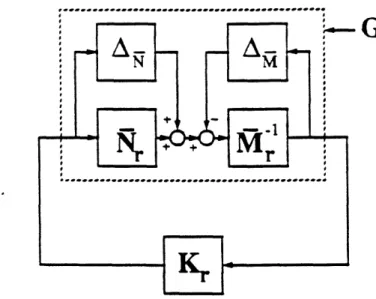
See Figure 1 for a block diagram of the closed-loop system. We recognise this system to be the one used to analyse internal stability [34, p101].

The LQG cost is then defined to be

C(X(G, K))

=

lim E{ 1t / z-(t)z(t) dt}

=lim E 2tf zT(t)CTC(t) + U(t)U(t)

t -oo j t!

where E denotes expectation.

Problem 3.1 (The Normalized LQG Control Problem) Find the controller K

which minimizes the LQG cost C( H(G, K)) over all stabilized closed-loops 7H(G, K).

Remark 3.2 It is easily seen that the Normalized LQG Problem has a 'standard plant' P (in the sense of e.g., [7]) given by

A BO] B

P21 P2 2

0

0 OO

[0

(6)

[C]

[

]

[0]

That is, [zT yT]T = p[wT uT]T where u = Ky. It is well-known [7] that a controller K stabilizes P if and only if it stabilizes P22, or since P22 = G, K stabilizes P if and only

if it stabilizes G. (By 'stabilizes' we as usual mean 'internally stabilizes'. That is ([5]), the states of G and K go to zero from every initial condition when w = 0.)

The solution to the Normalized LQG Problem follows from standard references [2,

18, 161.

Proposition 3.3 (Solution to the Normalized LQG Problem)

Let G = (A, B, C) be minimal. Then there exists a unique positive definite stabilizing solution X2 = XT E IRnXn of the control algebraic Riccati equation (CARE):

A4T2 + X2A - X2BBTX2 + CTC' = 0 C'ARE (7)

and there also exists a unique positive semidefinite stabilizing solution Y2 = yT E IRnxn of the filter algebraic Riccati equation (FARE):

U=Z2 Z1

K

Figure 1: Block diagram for the Normalized Problems

The Normalized LQG Controller KLQG = (A, B, C) takes the form of an optimal ob-server

= (A- Y 2CTC - BBTX2)± + Y 2CT y (9)

A B

together with the optimal state-feedback

u = -BTY 2 :. (10)

The minimum value of the LQG cost is

C(li(G, KLQG)) = trace[BTX 2B + BrX2Y2X 2B]. (11) Just as for ordinary balancing, under a nonsingular state transformation S, X2Y2 s

25 Since X2Y and STX2Y2ST are similar matrices, the eigenvalues of X2Y2

are similarity invariants. These invariants are the squares of the LQG-characteristic

values of the system G, as defined in [161; a formal definition and some basic properties

are given next.

Proposition 3.4 (LQG-balancing and LQG-characteristic values [16])

Let the system G = (A, B, C) be minimal -with n states and let X2 and Y2 be the

unique positive definite stabilizing solutions of the CARE and FARE respectively. Then the eigenvalues of Y2X'2 are real. strictly positive similarity invariants. as are their positive square roots which are called the LQG-characteristic values of G. Let 12 >

JL .. > _/2 > 0 denote the n. eigenvalues of X₂'2 arranged in decreasing order. then

there exists a similarity transformation which transforms both X.N and 12 to the form

M := diag(pl,,2, 2 .. . ,In,). The system is then said to be in LQG-balanced coordinates, and Al is the diagonal matrix of LQG'-characteristic values of G.

As argued in [161, in an LQG-balanced realization. small ui correspond to states which are easy to filter and control in an LQG sense. This motivates the following model reduction schemes.

Procedure 3.5 (Reduced-order plant by LQG-balanced truncation [16])

Let G = (A,B,C) be minimal with n states and in LQG-balanced coordinates

with LQG-characteristic values pl1 > p2 > . >._ P, > O. That is, M :=

diag(l,A2, ... , J,, ) = X2 = Y2 is the stabilizing solution of the CARE and FARE

associated with G = (A, B,C). Pick k < n such that Alk > PIk+l and partition M accordingly into

M=[ M1 0 ]

where M, = diag(Ilt,...,

,k)

and M2 = diag(&k+l,... ,n)). Partition A. B and C conformably with the partitioning of M:

A 2,1 A22 B = B2 and C= C₁ C₂ ]. A k-state reduced-order plant is then G, = (All, B1, C1).

Procedure 3.6 (Reduced-order controller by LQG-balanced truncation [16])

Let G = (A, B, C) be minimal with n states and in balanced coordinates with LQG-characteristic values 1 > It2 > ... I> An > O. That is, M := diag( 1,/ 2,..., t,) =

X2 = Y2 is the stabilizing solution of the CARE and FARE associated with G =

(A, B, C). Pick k < n such that Ak > /tk+l and partition M accordingly into

M = [M 02]

where MI = diag(tl,. .. ,uLk) and Ml2 = diag(/.k+l,.. .,,,). Let KLQG = (A,B,C)

be the Normalized LQG Controller for the plant G = (A, B, C) (as given in Proposi-tion 3.3). PartiProposi-tion A, B and C conformably with the partiProposi-tioning of M:

[

A21 2 ' B=[ and C= [ C C2 ]

,4 k-state reduced-order controller is then K, = (All,,, B1, C1).

Remark 3.7 The reduced-order controller

hK,

is the full-order Normalized LQG Con-troller for the reduced-order plant G,. This is an immediate consequence of the eas-ily seen fact that AllM is the stabilizing solution to the CARE and FARE for C, =

(All, B1, C ).

Of course, it is important to know what happens to the stability and performance of the closed-loop when a reduced-order Normalized LQG Controller is connected to the full-order system (.1, B, C). Sufficient conditions are derived in [16] for stability but these tend to be very conservative. since they give sufficient conditions for a dissipative closed-loop (further they only apply to the single-input single-output case).

4

7-,-Balancing and 7,--Characteristic Values

In this section, we show how all the results of the previous section can be generalized to the minimum entropy/'j-, case. See [251 for further details of the setup, the original definition of the 7',t-characteristic values vi, and their basic properties. The Normal-ized 4,O Control Problem on which the ",c-balancing method is based is simply the minimum entropy/7,t control problem associated with the system (4). The samle block diagram is appropriate (see Figure 1); the closed-loop transfer function is 'l(G, K) as before (see (5)). Some definitions and remarks are in order to begin with.

Definition 4.1 (.(G,y)-admissible controller) A controller K is said to be

(G,Y)-admissible if K stabilizes G and

II'(G,

K)I1, < 7.

Definition 4.2 ((G,-y)-admissible closed-loop) If K is a (G,y)-admissible

con-troller, then 'H(G, K) is said to be a (G, -y)-admissible closed-loop.

Remark 4.3 Each element of N(G, K) has a robustness interpretation, as follows.

(I-GK)-1 G corresponds to 'additive' uncertainty All on the controller K; (I-GK)-1GK

corresponds to 'output multiplicative' uncertainty A12on the plant G; K(I - GK)-'G

corresponds to 'input multiplicative' uncertainty A21 on G; and K(I - GK)- 1

cor-responds to additive uncertainty A22 on G. Block diagrams illustrating these four

uncertainty types Aij, i,j = 1,2, are provided in Figure 2. The upper bound 7 on II['(G, K)lt; implies robust stability guarantees for each of the four uncertainty types. This follows from the simple observation that

II(r - GK)-'Gl11o < 7

(I

- GK)-1G (I - GK)-<K <

II(Z

-

GK)-'GI

Itl

<

K(I - GK)-' G K( - GK)-1' - GK)-GII IIK( <"

11K(I

- GK)-1 tlI <

7

(12)

Using the Small Gain Theorem of [361 implies that closed-loop stability is maintained for any one Aij E Ztoo satisfying

IlaijllI

< -1, i,j = 1,2.

(Note that because K stabilizes G, we have (I - GK)-'G E .7-,,, (I - GK)-IGK E

1RZT , hK(I - GK)-'G E 47ZHo and K(I - GK)-1' 47',o.) If we use the Small Gain

Theorem on a frequency-by-frequency basis then a frequency-wise description of the tolerable Aij is obtained: closed-loop stability is maintained for any one Aij E R.7-, satisfying

al{All(j'c)} al{(I - G(jw)hK(jw))- G(jw)} < 1 Vw E IR.U {oo};

({A21(j2 _{.)} '1{(I - G(jw)K(jw))-'G(jwo)K((jw)} < 1 w E IRU {oO};}

71 {A21(jw) } a { ( jw )(I- G(jw)K(jw) ')- G(j w)} < 1 vw, IR U {oo};

o'l{A22(ju)}o '{K(jw)(I - G(jw)K( jw))-1} < 1 '~~ E IRU {oO}.

G

Additive uncertainty on K Output multiplicative uncertainty on G

AG ₁

I

K

Ka

Input multiplicative uncertainty on G Additive uncertainty on G

Figure 2: Uncertainty types Aij covered by the Normalized X', Problem

Let %, denote the smallest 7 for which a (G,-y)-admissible controller exists. Find-ing this 7o is an 'H,o-optimal control problem (see [7]). Throughout this paper we assume 7 > 0,. This permits the introduction of a minimum entropy criterion into the framework.

Definition 4.4 (Entropy) Let H E 14,, with H(oo) = 0 and

IIHIo.

< 7y. Then the

entropy of H is defined to be

2 0o

I(H, 7) := 2 In lnldet(I - -2 _{H'(jw)H(jw))l dw}

Note that if H is a (G, 7)-admissible closed-loop and G(oo) = 0 then we do have

H E R7ZO, H(oo) = 0 and

IIHIJI

< y.

Entropy minimization in the context of 1,,O control theory has been explored else-where (see [28, 26, 121). There are strong relations between minimum entropy/7'X con-trol and risk-sensitive LQG concon-trol (see [10, 9]), and also with the combined Ioo/LQG control considered in [3] (see [27]). However, due to lack of space we shall not elaborate further, except to quote the following result linking entropy with the LQG cost, which follows essentially from [28].

Proposition 4.5 ([28]) Let H E 7Z7-ko with H(oo) = 0 and

IIHIok

<

m.

Then

(i) I(H, y) = C(H) + O(7-2);

(iii) I(H, oo):= lim_.{I(H, y)} = C(H).

Remark 4.6 It is clear from Remark 4.3 and Proposition 4.5 that the Normalized 7-,

Controller guarantees a prespecified level of robust stability and provides a guaranteed LQG cost bound.

At last we may specify the problem of interest, which was introduced and discussed in [26].

Problem 4.7 (The Normalized X7,O Control Problem) Find the controller K

which minimizes the entropy [I(7'(G, K), y) over all (G, )-admissible closed-loops XH(G, K).

The solution to the Normalized H7/ Control Problem may now be stated, using the results of [5] and [12]. (In fact ([12]), the Normalized X7,0 Controller is the central

member of the class of all (G, y)-admissible controllers.)

Proposition 4.8 (Solution to the Normalized 7-,0 Problem)

Let G = (A, B, C) be minimal, and let 7 > ,0. Then there ezists a unique positive definite stabilizing solution X, =

XT

of the 7iH,o control algebraic Riccati equation

(HCARE):

ATX, + XoA - (1-

<-)Xo.BBTXo.

+ CTC = 0 HCARE (13) and there ezists a unique positive definite stabilizing solution YO = YT of the 73,o filter

algebraic Riccati equation (HFARE):

AY, + Y, AT - (1 - 2)YCTCY + BBT = O. HFARE (14)

There ezists a (G, y)-admissible controller if and only if there ezists positive definite X,Y, and Y,, as above, which satisfy Ama.(XoY,) < y2. Define

Z.o = ( -,- 2YX¥o)'. (15)

The Normalized 714, Controller KME.o = (A, B, C) takes the form of an observer

z = (A -(1 - -2)YooCTC BBT oZ ); + YC rT y (16)

A B

together with the state-feedback

u = -BTXZ' o. (17)

The minimum value of the entropy is

I(71(G, hKMEoo),) = trace[BTrX oB + BT Z,,rXoZoDoB]. (18) Although we are not concerned in this paper with 74o,-optimality, the following remark is worth noting: Corollary 5.5 should also be consulted.

Remark 4.9 By definition the 7-/o-optimal version of the Normalized X7-, Control

Problem is to find

7o = inf{ll7t(G, K)j11 : K stabilizes G}. Consider the closely related problem of finding

%f

:= inf{jlli(G,

K)llo

: K stabilizes G}, where

wr(G,K)

:= (GK)+ [0

0

(19)

This latter problem has an exact (non-iterative) solution [19, Remark 4.211 in terms of X2 and Y2, the stabilizing solutions to the CARE and FARE. respectively:

To = I1 + An.1 {X2Y2} > 1.

But the triangle inequality applied to the 7-oo-norm of (19) gives

II,(G,K)IIo

- 1 < I'l(G, K)Ioo <

IIl(G,K)llo

+ 1.

Taking the infimum over all K which stabilize G gives

0 < -1 <

-o

< _< + 1,

which provides (non-iterative) upper and lower bounds on y,.

Just as in ordinary balancing, under a nonsingular state transformation S, ,oYYo

-S-TJXoYoST, so the eigenvalues of XoYoo are similarity invariants, the positive square

roots of which we define to be the 7',o-characteristic values. All the arguments of Section 3 carry across and we obtain the following minimum entropy/7-o,o general-ization of Proposition 3.4. Note that since - > 70 by assumption, Proposition 4.8 gives Am,,a(XYoYo) < y2 so each of the H,o-characteristic values is strictly less than y.

Proposition 4.10 (H,o-balancing and X7,o-characteristic values [25])0

Let the system G = (A,B,C) be minimal with n states, let 'y > -y, and let Xo and Y} be the unique positive definite stabilizing solutions of the HCARE and HFARE respectively. Then the eigenvalues of XoYYo are real, strictly positive similarity invari-ants, as are their positive square roots which are called the XoH,-characteristic values of G. Let v1/ > V2 > ... > V2 > 0 denote the n eigenvalues of Xoo,ZO arranged in decreas-ing order, then y > vi and there ezists a similarity transformation which transforms both X-, and YO to the form N := diag(tv, V2, .. .,v,). The system is then said to be

in Hoo-balanced coordinates. and N is the diagonal matrix of 7H, -characteristic v'alues of G.

Note that the ',oo-characteristic values are functions of y. Strictly speaking, we should write 'i({y) and N(y). In the interests of notational simplicity, we will write vi and N.

The following proposition states some properties of the vi, and is included for com-pleteness.

Proposition 4.11 ([25]) For the vi as defined in Proposition 4.10 we have

(i) - > vi > tLi.

(ii) Each vi is a monotonically decreasing function of y. (iii) If the vi are distinct then dvl d-y < 0.

(iv) Each vi is a continuous function ofT. (v) lim_{li} = Hi.

5

Model Reduction by 7,oo-Balanced Truncation

As proposed in [25], reduced-order plants or reduced-order 7-oo controllers may be obtained by truncating those states in an 7t,o-balanced realization associated with small

h, O-characteristic values. This section gives a detailed analysis of this 7,H-balanced

truncation method of model reduction. It will be seen how -lo-balanced truncation is

an extension of LQG-balanced truncation to the minimum entropy/7Xo case. We will find, in contrast to model reduction using LQG-balanced truncation, that the a priori data 7 and the truncated vi are all that are needed to answer the questions posed in the Introduction, repeated here for convenience.

* How 'small' do the truncated Rio-characteristic values have to be to guarantee that a reduced-order controller stabilizes the full-order plant?

* What is the degradation in performance caused by using a reduced-order controller in place of the full-order controller?

Answers to these questions are contained in Section 5.4.

5.1 7-H,-Balanced Truncation

Procedure 5.1 (Reduced-order plant by '7,--balanced truncation [25])

Let G = (A, B, C) be minimal with n states and in oHo-balanced coordinates for given 7 > >'2 z,, with 'too-characteristic values y > >_ Ž ... > v, > 0. That

is, N := diag(vl ,w2,..., L,) = Xoo = Y,o is the stabilizing solution of the HCARE and

HFARE associated with G = (A,B,C) and -y. Pick k < n such that vk > vk.l and partition N accordingly into

L O V

N

where .V1 = diag(v1,.... ,k) and N2 = diag(vk+l, .... v,n). Partition .4. B and C'

conformably with the partitioning of N:

[ 21 22

B

=

B2

and

C

C'1

C2

.4 k-state reduced-order plant is then G = (All, B1, C').

Procedure 5.2 (Reduced-order control by X7-,-balanced truncation [25])

Let G = (A, B, C) be minimal with n states and in -t,,0-balanced coordinates for

given y, > 7,, with 'tI,-characteristic values 7 > vl > v,2 > ... > ,vn > O. That

is, N := diag(vl, v,... v,,) = X', = Yo, is the stabilizing solution of the HCARE and HFARE associated with G = (A,BC) and y. Pick k < n such that vk > Vk+l and partition N accordingly into

N=[l0 N2

where N1 = diag(vl,...,vk) and N2 = diag(vk+l,...v,). Let KMEOO = (A,B,C)

be the Normalized X7i' Controller for the plant G = (A, B, C) and 'y (as given in Proposition 4.8). Partition A, B and C conformably with the partitioning of N:

A l l A12

1]

A= [

l

2 | B=[ B and C=[C C2 ]

.4 k-state reduced-order controller is then K, = (A 1, B1, C1).

Remark 5.3 The reduced-order controller K, is the full-order Normalized 7',0.

Con-troller for the reduced-order plant G,. This is an immediate consequence of the easily seen fact that N1 is the stabilizing solution to the HCARE and HFARE

for G, = (A11, B1, C1).

We can now relate the H,-characteristic values of G to the Hankel singular values of G.

Proposition 5.4 ([25]) Suppose G = (A, B, C) is asymptotically stable and minimal,

with Hankel singular values al O > 2 > ... > a, > O. Let - > 70 and let G have oL,,-characteristic values 7 > 1 v> 2 > ... > , > O. Then

(i) If > 1 then cri > vi.

(ii) If 7 = 1 then ai = vi.

(iii) If y < 1 then ai < vi.

Proof The following proof is taken from [25], and is included for completeness. Note

that (A, B, C) is not necessarily a balanced realization of any type. The controllability Gramian P = pT > 0 and observability Gramian Q = QT > 0 are given by

AP + PAT + BBT = 0 (20)

ATQ + QA + CTC 0. (21)

and then

j

= ¾QP}.

Subtract the HFARE from (20), and subtract the HCARE from (21):

A(P - Y o) + (P - Y.)AT + (1 - )Y-: C.TCYo = 0 (22)

Part (i) By assumption, A is asymptotically stable and 1 - y- 2 > 0. A standard result on Lyapunov equations (see [8, Theorem 3.3(7)]) applied to (22) and (23) then gives P > Y,, and Q > XS. Hence, by the argument in the proof of Proposition 4.11(i),

Ai{QP} > Ai{XYo} }. Recalling cr = \i{QP} and v2 = AI{XY }, the result follows. Part (ii) Put 7 = 1 in (22) and (23):

A(P - ',) + (P - Y )AT = 0 AT(Q _ X o) + (Q-XoX,)A = 0.

Since A is asymptotically stable by assumption, it follows from [31] that P = Y,. and Q = Xoo. Hence the result.

Part (iii) The same argument as used to prove Part (i) may be applied, except

now 1 - a-2 < O0. It follows that P < Yo and Q < XY,, which implies the result. a3 Corollary 5.5 Suppose G = (A, B, C) is minimal. Then y, < 1 if and only if G is asymptotically stable and has Hankel norm cr < 1.

Proof If Suppose G is asymptotically stable and has Hankel norm cl < 1. Then the controllability Grainian P = pT > 0 and the observability Gramian Q = QT > 0 satisfy (20) and (21) respectively, and A,,az(QP) =

al

< 1. Setting y = 1, from the proof of Part (ii) of Proposition 5.4 we have P = YO and Q = Xo,. Hence

Proposition 4.8 implies that there exists a (G, 1)-admissible controller. So -y, < y = 1.

Only if Suppose y, < 7 < 1. Then (14) can be written as a Lyapunov equation:

0 = YoAT + AYo + [aYoCT BI[aYoCT BIT,

where Ca2 := 7- 2 - 1 > 0. The pair (A, [aY.CT B]) is certainly stabilizable because, by assumption, (A,B) is controllable. This together with Y,, > 0 implies that A is asymptotically stable, using a standard result on Lyapunov equations [35, Lemma 12.21. Finally, combining Parts (ii) and (iii) of Proposition 5.4 gives Oal _ v < 1. [] Remark 5.6 From Proposition 4.11(v) we see that if the 7H,O-norm bound 7 is re-laxed completely i.e., Y - oo, the '7,o-characteristic values become precisely the

LQG-characteristic values. Indeed, Proposition 4.5(iii) implies that in this case the Normalized H,,O Control Problem becomes the Normalized LQG Control Problem. So the results of Section 3 on LQG-balanced truncation could all be viewed as limiting cases of the results on 1o,-balanced truncation.

5.2

Coprime Factorization via the Normalized 7-, Problem

A key step in the analysis of 2,o-balanced truncation will be to link it to balanced truncation of the normalized coprime factors of a scaled plant. To be specific. consider the scaled plant 3G where

For /3 to be well-defined we assume -y > max{1,yo} so that 0 < 3 < 1. This is not a severe restriction; Corollary 5.5 shows that yo < - < 1 is possible if and only if G is asymptotically stable and has Hankel norm less than one.

Balanced truncation of normalized coprime factors has been considered in [21] and [19, Chapter 5]. The idea is as follows. Let L3G = M1-'3V be a normalized left-coprime factorization. That is.

(i) ON E ~7Z, and M E 17Xo;

(ii) 7M is non-singular;

(iii) /3NV and M are left-coprime (i.e., 3BX,Y Y E 77-I, s.t. ,3UNf +

MYf'

= 1); (iv) 32 VNN* + MM* = I;

(v) /G= M-1,/3N.

In the above, item (iv) is the normalizing condition.

The matrix ([{N .I] is asymptotically stable and hence balanced truncation may be applied to obtain reduced order coprime factors [3N, 37I,. The detail will be provided in the next subsection. Before that we must show how to construct [/3N 17f] and write

down its Hankel singular values, all in terms of quantities we already have available from the Normalized iO Problem.

The first step is to use [22] to construct the normalized left-coprime factorization of 3G using one of the 74,O algebraic Riccati equations of the Normalized Noo Problem.

Lemma 5.7 Let G = (A,B,C) be minimal and let 7 > max{1,y0}. Let /3 = (1 -,- 2)1/2. Let Ye be the unique positive definite stabilizing solution of the associated

HFA RE. Define N and ill by

[o/3~' g=

,}}

[-

A CB 0 '= (24)

Then

(i) /G = - M-'IN is a normalized left-coprime factorization of/3G.

(ii) The controllability Gramian of [p3N Ai ) is p = /32yoo,

and the observability Gramian of [3iN A11] is Q = (o -- 1 d2+)-I

(iii) Let l > &2 > ... > an > 0 be the Hankel singular values of [/3N AI]. Let y > vl > v2 >_... > v, > 0 be the X',-characteristic values of G. Then

- = 2"32

Proof Appendix A. a

Remark 5.8 From [29, 231, the realization (24) of [3fi3V ]f is minimal if and only if

the realization G = (A, BC) is minimal. Minimeality of G = (A.B.C') is a standing assumption in this paper.

Remark 5.9 Suppose [03N JM] is in balanced coordinates. Then its controllabil-ity Gramian P and its observabilcontrollabil-ity Gramian Q satisfy P = Q = v _{where ~ =}

diag(a₁, &2, ... , an) is the balanced Gramian. But then from Lemma 5.7(ii), Y,2 = _3-2: and XO = (S-1 _ )-', which are both diagonal, with product

oYo =' -:(g-1 _)-1l

= diag(/3-2(1 _ a2)-l, 3-2 _{2(1 _ &2)-1,. ,-2&2(1 _ 2)-)}

-diag(v21, v2 ) -N 2,

using Lemma 5.7(iii). Thus. G may be put into Xo-balanced coordinates by applying the diagonal state similarity transform

i31/2(1 _- f2)-(1/4)

(which was derived in a straightforward way by applying the method of [8, Section 4]).

Remark 5.10 Suppose G is in 74Ho-balanced coordinates. Then Xo = Y, = N where

N = diag(vj,v 2 ,..., V,). But then from Lemma 5.7(ii), P = ,32N and Q = (N-' +

/2N)-', which are both diagonal, with product

PQ ,32N(N-1 + 32N)-'

= diag(3 2v2( 1 +/3 2v1)-1 2 v,2(1 + 2v2)- 1 -3. 32v2(1 + o2 2 )-1

S -2

using Lemma 5.7(iii). Thus, [3N t1IV] may be put into balanced coordinates by applying the diagonal state similarity transform

/3-(1/2)( + - 2N 2)-(1/4),

(which was derived in a straightforward way by applying the method of [8. Section 4]).

5.3

Model Reduction via the Coprime Factors

We are now in a position to carry out balanced truncation of the normalized left-coprime factors [/3N Mf] of the scaled plant3 G, to obtain a reduced-order plant. The analysis here and in the next subsection is reminiscent of [19. Chapter 5].

Procedure 5.11 (Reduced-order plant by coprime factorization of L3G)

Let G = (A,B. C) be minimal with n states and let y > max{ 1,y 0}. Let 3 = (1 - -2)1/2. Let 3G = if-13l3N be the normalized left-coprime factorization

of fiG based on the HFARE-that is, let [,3N Vifi = (AB, , D) be as given in Lemma 5.7. Let the state-space realization of [iN

Mf]

be in balanced coordinates

with Hankel singular values 1 Ž &2 > > .2 .. > > O. Pick k < n such that Ok > &k+l and let [i3N, Mil] := (Al1, B1, Cl, D) be obtained by balanced truncation of [(3N fM]

to k states (Procedure 2.2). Then a k-state reduced-order plant is G, := ;'lN and [23] G0, =

M

3r-liNr, is a normalized left-coprime factorization.

How does this reduced-order plant compare with the one obtained via 7-,"-balanced truncation in Procedure 5.1? The next result answers this question.

Theorem 5.12 The plant model reduction schemes described in Procedure 5.1 and Procedure 5.11 yield identical reduced-order plants. To be precise, let G, be the k-state reduced-order plant obtained by performing 7-',,-balanced truncation (Procedure 5.1) on the full-order plant G for y > max{1, 7}. Let G, be the k-state reduced-order plant obtained by performing balanced truncation of the coprime factors [OfN

MfI]

of fiG (Procedure 5.11) where /3 = (1 - 7-2₎1/ 2_{. Then}

G, = G,.

Proof Suppose G = (A,B, C) is 7,4-balanced, and we form G, by X7-/-balanced

truncation. Thus, according to Procedure 5.1, we have the partitioning

X,=Y

=NY. =[ZN

0N]

0 IV2

where N, = diag(vl,..., vk,) and VN2= diag(vk+l,..., v,,), together with

A

A122 =[ =

B2

and C

[ C1

C2

]

The k-state reduced-order plant G, is then

G, =A[ B1 (25)

Using Lemma 5.7, we can use N to construct the normalized left-coprime factoriza-tion 3G = .I'-'/3N (with the partifactoriza-tioning corresponding to that of N made explicit):

11 -3 2NVC' CI -'12 - .32 _Cf'

2 3B, -. 32VC'

[031V

1i]

=

1

- 32 CV2C

A22

- 32N_{2 C}2TC2 B₂ ,32

N

₂

CT

, (26)

C, CC2 0 I

with Gramians P = 32N and Q = (N-' + da2N)- 1. But from Remark 5.10, this may be put into balanced coordinates by a diagonal state-transformation. Denote this diagonal balancing transformation by L = diag(L1, L2), partitioned conformably

with iV = diag(NV1, V2). (An explicit expression for the balancing transformation L

is given in Remark 5.10 but we shall not need it.) Applying this diagonal balancing transformation to (26) gives

L1AllL- 1 LiAi2L- 1 I L1B -_2LIVICT

[0V IV] = L2A21L-1 L2A2 2L'2 jL 2B2 -d2L 21N2CT

CL 1 C2Lll 0 I

where Aij := Aij- 32NiC Cj, i,j = 1,2, which is a balanced realization with

(Re-mark 5.10) balanced Gramian E. Applying Procedure 5.11, the k-state reduced-order plant 0, has a normalized left-coprime factorization 30, = 'f'r-l3N, where [iN,

MI,]

is obtained by balanced truncation of [AIN M]. Thus, truncating the above balanced realization to k states, [/3N,. ll] =

[

L1(AL-3 2N1 CTC1)L' I /3LB 1 -3 2LiNCT ]1N CL-' 0 I =A[AI - 32N₁Cl C 3B₁ -3 2NjC=T C1 0 IC C,. z= Ml7l:%r'

=

K

Ah

a

But this is precisely G, in (25). a

The following corollary is immediate on taking note of Remark 5.3.

Corollary 5.13 Let K, be the k-state reduced-order controller obtained by performing 7to,-balanced truncation (Procedure 5.2) on KMEO,, where KMEoo is the full-order Nor-malized .,O Controller for the full-order plant G. Let A, be the k-state Normalized

iH, Controller for the k-state reduced-order plant G, (Procedure 5.1 or equivalently Procedure 5.11). Then

K,= -,.

It is therefore irrelevant whether we consider doing model reduction by 7H,-balanced truncation before or after the control; there is a compatibility between the closed-loop objectives of Normalized 7-00, Control and model reduction by 7,o-balanced truncation.

5.4

Stability and Performance with the Reduced-Order

Con-troller

We can now piece together results from the previous sections to consider the stability and performance of the closed-loop consisting of the reduced-order Normalized 7Ho. controller K, with the full-order plant G (as illustrated in Figure 3). It is an advantage of using Xi,-balanced truncation that the results may be expressed in terms of a priori quantities only (i.e., 7/ and the neglected vi). This comes about because the model reduction error e defined by

Oi3 :=-11[/3, X.H]{, (27)

where

AN := N?- :N,

A~Q :=

M

-

Air,

may be bounded above using y and the neglected vi only. To be precise, the balanced truncation error bound of Lemma 2.3(iii) applied to (27) gives an upper bound on ,3 in terms of the neglected Hankel singular values of [,/N ITJ. Hence, from Lemma 5.7(iii),

d3 may be bounded in terms of the 7O4,-characteristic values of G:

< 2 trace[ ₂ = 2 : v 2 (28)

i=k+I/1 +

Therefore,

<2Z

2a

(29)

i=k+l 1 + /32v2 and by inspection, a weaker but simpler bound is

!

< 2 E vi = 2 trace[lV₂]. (30)

i=k+l

This last upper bound is 'twice the sum of the tail,' just as in ordinary balanced truncation (Lemma 2.3(iii)). Using either of the above upper bounds in place of e

in the following results gives a (conservative) statement of closed-loop stability and performance using the order controller without having to calculate the reduced-order controller in advance.

Proposition 5.14 Let K, be the k-state reduced-order controller obtained by

perform-ing '7',-balanced truncation (Procedure 5.2) on the full-order Normalized 74, Controller for the full- order plant G with 7 > max{1,y₀}. Let iG = iM-1/3N be the normalized left-coprime factorization of /3G given in Lemma 5.7. Let flG, = MTIf-7/3Nr be the nor-malized left-coprime factorization (Procedure 5.11) of the k-state reduced-order plant G, obtained by performing 74, -balanced truncation (Procedure 5.1). Let

Kr =Ur

.

-be any right-coprime factorization of K,. Define r,:= A, ;Vr RU.l

Let e be the model reduction error as defined in (27) above. Then the condition

i/13 ]R-1

< 1

ensures closed-loop stability of the system consisting of the reduced-order controller IK. and the full-order plant G.

Figure 3: Reduced-order Normalized 'H,O Controller with full-order plant

Proof The proof is basically an application of the Small Gain Theorem. Rather than repeat the argument here, we will for brevity quote a result [19, Corollary 3.7] which, for our case, states that K, stabilizes G if K, stabilizes G, (which it does by construction) and

where S, := (I - G,K,)- '. The claim of the proposition follows easily on making the necessary substitutions to obtain

S,, = ~V R;-.Mqf (31)

and then

/r S,, - 1 = U rr

Corollary 5.13 shows that K, is in fact the normalized 17o controller for G,. Define

:= 7-(Gr,.Kr)11f, (32)

to be the actual ',o-norm of 7'-(G,,hKr). Then

< '¥ (33)

is immediate, and the following corollary to Proposition to .5.14 is obtained.

Corollary 5.15 With definitions as above, we have that

R-[1~

U]R

<S+f,

(34)

so the condition

(0 + i) < 1

is sufficient to ensure closed-loop stability of the system consisting of the reduced-order controller K, and the full-order plant G.

Proof Appendix B. 0

Remark 5.16 An a priori test for the stability of the system consisting of K, with G

is immediate. Just replace -y with its upper bound 7 (equations (32) and (33)), and replace e with e, where e is an upper bound on c, such as that given in (29). It is simple to verify that

( +) < 1 . (+) < .

Hence to test if K, stabilizes G it suffices to check if e(/3 + y) < 1, a simple test which depends only on - and the truncated vi.

Now assume that i(,/3+j) < 1 so that, by Corollary 5.15, the closed-loop consisting of the reduced-order controller K, and the full-order plant G is stable. From Remark 4.3 we know that the bound II'H(G, KMEO.)l[.O < 7 inherent in Normalized X7, Problem gives robust stability guarantees. The next proposition tells us how much the bound

II7/(G, KhME.O )IIo < 7 is degraded (increased) by using the reduced-order controller K, in place of the full-order Normalized 7'H0 Controller KMEoo.

Proposition 5.17 Definitions as above. Assume i(/3+f) < 1 so that the reduced-order controller Kh; stabilizes the full-order plant G. Then the associated closed-loop transfer function satisfies

II /(G,KE,)1lo. __< + ~(l + j)(1 7)^(p+ ) (35)

Proof Appendix C. [

Remark 5.18 An a priori upper bound on

II7-(G,

K,)l[oo is immediate from (35). Just

replace - with its upper bound 7 (equations (32) and (33)), and replace e with e, where e is an upper bound on e such as that given in (29). Provided that e(3 + Y) < 1, Remark 5.16 predicts that K, stabilizes C. Under this condition. it is simple to verify that the right-hand side of (35) can only increase on replacing e with e and ' with -y.

That is,

( ,K)

<+E (1 + y)(l + 3 + )(36)

(1 - e(/3 + 7))

which depends only on 7 and the truncated vi. So in this context. the n - k smallest

vi are 'small enough' to be discarded if e(/3 + y) < 1. Beyond this. smaller discarded vl lead to a better reduced-order controller; 'better' in that the upper bound (35) is

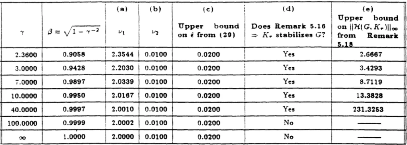
(a) (b) (c) (d) (e) Upper bound Upper bound Does Remark 5.16 on ,H(G,K.)JI

B VI>2on = e from (29) K- K. stabilizes G? from Remark

2.3600 0.9058 2.3544 0.0100 0.0200 Yes 2.667 3.0000 ) 0.9428 2.2030 0.0100 0.0200 Yes 3.4293 7.0000 0.9897 2.0339 0.0100 0.0200 } Yes 8.7119 10.0000 0.9950 2.0167 0.0100 0.0200 Yes 13.3828 40.0000 0.9997 2.0010 0.0100 0.0200 Yes 231.3253 100.0000 0.9999 2.0002 0.0100 0.0200 No .00.00 2.0000 0.0100 0.0200 No

Table 1: 7-,o-balanced truncation example: a priori numerical results

Remark 5.19 Note that as 7 increases. the a posteriori result of Proposition 5.17 re-mains viable, whereas the a priori result of Remark 5.18 becomes increasingly weak. In the limit as 7 -x oo (the LQG case), Proposition 5.17 is still viable, whereas Re-mark 5.18 becomes vacuous.

Remark 5.20 Note that if the model reduction error -i 0, the upper bound (35)

recovers the definition ~ = ll1(G,,K,)llj,. Similarly, the upper bound (36) recovers the full-order bound 1ItI(G, KMEo)oI < -' if the model reduction error bound E -- 0.

5.5

A Numerical Example

The results derived above are illustrated here using a numerical example. Consider the system

G = _A A3/4 _{B -}

[

_{98/201 -9999/200} -98/201 1₁

[

61 = 1 0

This system was constructed in [16, Section VIII to be in LQG-balanced coordinates with LQG-characteristic values tl, = 2.0000 and JL2 = 0.0100. To verify this, one merely

has to check that M = diag(pl,/A2) is the stabilizing solution of the CARE and FARE. The system has a left-half plane zero at -24.1349 and poles at 0.7547 and -49.9997.

Using y-iteration gives 7o = 2.3559. We chose seven representative values of 7 > y, at which to perform X7,-balanced truncation: ' = 2.36. 3, 7, 10, 40, 100 and oo.

The results are tabulated in Tables 1 and 2: the 'predicted' results in Table 1 and the 'actual' results in Table 2. We know that when -- . the R7-,-balancing method recovers the LQG-balancing method (see Remark 5.6). This is confirmed in Tables 1

and 2, where the last row (corresponding to y, - oo) of Columns (a), (b) and (i) agrees with the results of [16. Section VIII.

For each of the chosen values of 7, the HCARE and HFARE are solved and the 'Lo-characteristic values are calculated using Proposition 4.10. This gives Columns (a)

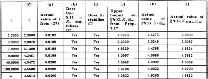
(f) I (g)(h) I (i) I (j) (k) ()

A

Does K Upper

Actual Cor. Does K, bound on Actual

5.15 Actual value of

v

i~

~ of i Kvalue sta- stabilize II7/(G,K,)IIo value of from (27) bils G? from Prop. JI((G,K,) jKMjoo

5.17 2.3600 2.3600 0.0182 Yes Yes 2.6373 2.4273 2.3600 3.0000 2.9076 0.0189 Yes Yes 3.2939 3.0249 2.9087 7.0000 4.1396 0.0198 Yes Yes 4.8339 4.4268 4.1524 10.0000 4.3451 0.0199 Yes Yes 5.0997 4.6688 4.3612 40.0000 4.5472 0.0200 Yes Yes 5.3642 4.9092 4.5669 100.0000 4.5590 0.0200 Yes Yes 5.3794 4.9233 4.5790 oo 4.5612 0.0200 Yes Yes 5.3823 4.9260 4.5812

Table 2: 7X,-balanced truncation example: exact and a posteriori numerical results and (b) of Table 1. For each choice of

-

we have vl > v2, which prompts us to

con-sider obtaining single-state reduced-order controllers by discarding v2 via 'X,-balanced truncation (Procedure 5.2). But before calculating the reduced-order controllers, we can predict their success using the a priori data - and v2. Using (29), an upper bound on the model reduction error e may be calculated from the neglected v2, giving

Col-umn (c). As explained in Remark 5.16, this upper bound on e may then be used in

place of e in Corollary 5.15 to predict stability of each reduced-order controller hK, with

the full-order plant G, Column (d). Notice that stability of K, with G is predicted for all but the two largest choices of 7, when nothing can be deduced. In the cases where stability of K, with G is predicted, the performance of that configuration can be bounded using Remark 5.18, as shown in Column (e).

Having predicted the satisfactory behaviour of the reduced-order controllers we can go ahead and calculate them using Procedure 5.2, from which Table 2 is constructed. The model reduction error e may be calculated exactly from (27) using the algorithm

in [4], to give Column (g). Stability of K, with G may be tested for explicitly by calculating the closed-loop poles, to give Column (i). The actual 7t,-norm of the closed-loop of K, with G is also calculated explicitly using the algorithm in [4], to give Column (k). Likewise, A, the actual 7X,-norm of the closed-loop of IK, with G,, is calculated explicitly to give Column (f). For reference, in Column (1) we give the full-order results, that is, the actual 7',O-norm of the closed-loop 7'(G, KME.o) consisting of the full-order controller KMEoo with G.

Using the a posteriori data j and i, Corollary .5.15 may be used to check if stability of fK. with G is predicted, see Column (h). Proposition .5.17 then allows calculation of an upper bound on the XO,-norm of the closed-loop of K, with G (Column (j)). Notice that it is predicted that K, stabilizes G for all the values of y, including infinity. Also, the upper bound in Column (j) is within 10% of the actual value in Column (k), again even for large 7.

Comparing the two tables of results it is clear that the 7',o-balanced truncation method can give a good reduced-order controller. Furthermore. when y is small (of the

order of o), indicating a preference for robustness over LQG performance, the 70-balanced truncation method gives accurate a priori prediction of the performance of IK, with G. This is particularly clear on comparing the first three rows of the two tables. Using the a posteriori data 7 and I, even tighter results are possible: they indicate that

a good reduced-order controller can be obtained even when y is large (in which case the

a priori predictions may be weak, as indicated in Remark 5.19). This is particularly

clear on comparing the final three rows of the two tables.

6

Conclusions

',o.-balanced _{truncation has been analysed here as a method for deriving} reduced-order plants or reduced-reduced-order 7,/ controllers. An easily tested criterion for the ability of such a reduced-order 7/,, controller to stabilize the full-order plant was derived. The criterion required knowledge only of the prespecified X7o-norm bound and the discarded 7o,-characteristic values. Then we derived an upper bound on the Xoo-norm of the closed-loop consisting of the reduced-order 7'/00 controller and the full-order plant. That too relied on the same a priori data. ,o-balanced 0 truncation is one of the few known

methods where such a priori results exist for the reduced-order controller. The results arise because of the compatibility between the reduction procedure and the closed-loop objectives. Another problem where a priori results are possible is the coprime factor problem in [20].

Computationally the 7oo-balanced truncation method is very simple, since the 7/.-characteristic values are easily calculated from the solutions to the design Riccati equa-tions in advance of doing any model reduction. This was seen in the numerical example. In [30], it was shown that the LQG-balancing approach is particularly applicable to symmetric passive systems, such as large space structures with colocated rate sensors and actuators. We would expect this to be the case for the 7H,-balancing approach too, and it would be instructive to compare results. However, as pointed out in [30, p831, for systems with no symmetry or passivity properties, a non-normalized approach may be more suitable. One possible way round this would be to apply the normalized approach not to the actual plant, but to a 'shaped' plant which has been (open-loop) pre- and post-compensated. The success of such 'loop-shaping' ideas has been demonstrated in [19], using controller synthesis via the robust stabilization of the normalized coprime factors of a plant. It would be interesting to apply and analyse such loop-shaping ideas in the context to -oo-balanced truncation.

A

Proof of Lemma 5.7

Part (i) Multiply the HFARE by d2 and define } := 32Y. Then

WAYS Y~Ar Y-YCTrCi + (dB)(13B)T = 0.

Using this equation the required normalized left-coprime factorization of d3G

(A, 3B, C) may be written down immediately using [11. Lemma 2.1].

Part (ii) The controllability Gramian P = pT is the unique positive definite solution to the Lyapunov equation

P(A - IO2yooCTC)T + (A _ 32YCTC)P + 2BBT + 3 4yoCTCyo = 0.

It is easy to show. using the HFARE, that P = 32Yo solves this equation.

The observability Gramian Q = QT is the unique positive definite solution to the Lyapunov equation

Q(A -

3

2_{YooCC) + (A}

-32YooCTC)TQ + CrC = 0.

Pre- and post-multiply by Q-l and substitute Q-' = X 1_+f 2_{Yo, (XYl exists because}

XO > 0 from Proposition 4.8.) It is then straightforward to use the HFARE and the HCARE to show that the equation is indeed solved by this choice of Q.

Part (iii) Firstly recall the definitions 2 = A1{QP} and v2 = Ai{Xo,' o}. Then,

using Lemma 5.7(ii) to express P and Q in terms of S, and Yo, we have

. = Ai(QP}

= A1 {((xl + 2 y, )-132Y }

=

A;{(I

+ :32 _XY0,)-13 2_{X, ¥o}}

_= 2 Ai{X(oYoo

}

1 + /32Ai{XoYo}

1 + /32V

B

Proof of Corollary 5.15

We only have to prove that (34) holds: the corollary follows immediately from that and Proposition 5.14. Now, K, is the Normalized 7'H Controller for the plant G,. The closed loop transfer function is

7(G,,K,) = KS, G, K, S,,

where S,, := (I - G,K,)-l. We need to rewrite this closed-loop transfer function in terms of the coprime factorizations G, = ll

Y,.r

and K, =

U,1j'

- _{'. We have}

R..

,

=

I,

I';

-

*Yr,

by definition and

from (31). Straightforward manipulations then give

H(G.,)= [ S Gr Srr

[

]

-

VR-l

V,

VrfRs

-

1

_O

_I

= U, Rr'N-, LR -lM, L

V, rr 0 I

[U.]R;'[Nr M

]

t [go

O]|

Hence

[Ur ]R-1l. [

M= + -H(G,

;r)

(37) and [U, j R [ Nr r ] [ I] (3[ ° ° ]jGKr)) (38) Similarly, [U]R.

]

[3 r

r]=([O ] +H(G,K))[ I ] (39) and also

Ur

]

[

1I]([

oo]

0)

[

0

]

[ °v °

,

[

O

I ]

(G:t

·

[

I*

(40)

Take the lH,_{0-norm of (37)-(40) and use the triangle inequality and the} sub-multiplicative property of the 7,O-norm. Also use that j[iH(Gr, K,)1[oJ =

5

by definition and that 0 < / < 1. Then

[. ]R;[Nt M ] < 1 + (41)

and

3[ VrI RrI[r a[], <3 +. (42)

Also.

[

];r

]r[

'

M

]

=4

[

jRrr|

< 1

+,

(43)

and finally

[I j ]Rrr [3N. Mt

V

]

[s

Ir3

]

Rrr1

<

±.3

+

(44)

The first equality in (43) and in (44) arises because [13Nr, fI,] is normalized. Equa-tion (44) is (34) as claimed; equaEqua-tions (41)-(43) will be needed in Appendix C. O]