Constraining the North Atlantic Circulation with
Transient Tracer Observations
by
Xingwen Li
Submitted to the Joint Program in Physical Oceanography
in partial fulfillment of the requirements for the degree of
Doctor of Philosophy
at the
MASSACHUSETTS INSTITUTE OF TECHNOLOGY
and the
WOODS HOLE OCEANOGRAPHIC INSTITUTION
February 2003
@Xingwen
Li, 2002
The author hereby grants to MIT and WHOI permission to reproduce
paper and electronic copies of this thesis in whole or in part and to
distribute them publicly.
Author ...
Joint Program in hysical Oceanography
Massachusetts Institute of Technology
W99ds Hole Oppanographic Institution
October 30, 2002
Certified by...
. . .
.
.
. .
Carl Wunsch
Cecil and Ida Green Professor of Physical Oceanography
lfssac4iuset( Institute of Technology
Thesis Supervisor
Accepted by ...
...
Carl Wunsch
Chairman, Joint Committee for Physical Oceanography
Massachusetts Institute of TechnologyMASSACHUSETTS INSTITUTE
Woods Hole Oceanographic Institution
NA
LINDGREN
Constraining the North Atlantic Circulation with Transient
Tracer Observations
by
Xingwen Li
Submitted to the Joint Program in Physical Oceanography Massachusetts Institute of Technology
Woods Hole Oceanographic Institution on October 30, 2002, in partial fulfillment of the
requirements for the degree of Doctor of Philosophy
Abstract
The capability of transient tracers to constrain the ocean circulation in the North Atlantic is explored. Study of an idealized tracer shows that inferences of circulation properties from transient state distributions are impacted by uncertainties in the time-varying boundary conditions and sparse data coverage. Comparison of CFC, tritium, temperature and salinity (T-S) observations with model results in the North Atlantic shows that regions of important model-data disagreements in the transient tracer fields can also be readily identified in the T-S distributions. In the model, excessive vertical penetration of convective adjustment, leads to problematic production and outflow of the NADW, again appearing in both transient tracer and T-S fields.
Sensitivities of the model fields are determined using the adjoint model. In the dual solutions, CFC-11, CFC-11/CFC-12 ratio age, and T - (3/a)S (oz and
#
are thermal and haline expansion coefficients, respectively) exhibit the major ventilation pathways and the associated timescales, in the model. High sensitivity fields are candidates for providing the most powerful constraints in the corresponding inverse problems. Assimilation of both CFC and tritium data, with different input histories, sampling distributions, and radioactive decay constants, shows that by adjusting only initial-boundary conditions of CFCs and tritium, a 1 x 1" offline model and the transient tracer data can be brought into near-consistency, in the domain between 4.5"S and 39.5"N of the North Atlantic.Constraining a GCM with transient tracers is thus fully practical. However, the large uncertainties in the time-varying boundary conditions of transient tracer concen-trations, and in their interior distributions, renders the transient tracers less-effective in determining the circulation than are more conventional steady tracers, and known oceanic dynamics.
Title: Cecil and Ida Green Professor of Physical Oceanography Massachusetts Institute of Technology
Acknowledgments
I would like to extend my sincere appreciation for all the assistance and support that
I got throughout this thesis and my years at both MIT and WHOI.
First and foremost, I would like to thank my supervisor, Carl Wunsch, who pro-vided me with invaluable time, resources, advice and financial support. His insight, integrity, enthusiasm and disposition are good sources to benefit my whole life. I felt incredibly fortunate to have a prominent advisor, who responded to my questions and results in time, who patiently read numerous drafts of this work, which made working on this thesis an enjoyable and exciting experience. His constructive comments and suggestions were essential to this thesis.
I thank the other members of my committee, Nelson Hogg, Glenn Flierl, Michael Follows and David Glover. Their doors were always open for questions and discus-sions. They carefully read many drafts of this thesis, made valuable comments, and helped me go through theoretical and technical problems at various stages of this work. Michael Follows explained the essential details of the adjoint modeling to me. Thanks also go to the other members of the physical oceanographic group at MIT and WHOI who provided me assistance.
This work was supported by NSF Award #OCE-9730071 (A Synthesis Of The Global WOCE Observation), #OCE-9617570 (Estimating The Climatological Annual Cycle), and by NASA Award #NAG5-7857 and #NAG5-11933 (A Synthesis Of The Global WOCE Observation).
I am grateful to all the investigators who allowed me to use their data, either directly or through the WHPO. Thanks in particular to Scott Doney, Thomas Haine, John Bullister, Bill Smethie, Wolfgang Roether, Martin Gould, Laurent Memery, Peter Schlosser, and Samar Khatiwala. Scott Doney also provided necessary data and associated scripts for computing the CFC age and tritium distributions.
I felt very lucky that I studied among very nice classmates. I thank Geoffrey Gebbie for his valuable discussions with me about study and research problems, and for being my sincere counselor about cultural and academic problems. Much gratitude
goes to Baylor, Peter, Kerim, Payal, Avon, Allison, Heather and Zan for creating a warm and friendly atmosphere. Special thanks go to Susan Spilecki for helping me improve my writing skills. I thank Liangjun, Youshun, Yufei and Zhoutao for sharing good times and opinions with me. I thank Xiaoyun and Yong for helping me settle down when I first came to the States. Thank you, Xiaoou; Qiao and I had a good time here. Thanks go to Xin Huang for his introduction to the MIT/WHOI joint program.
This dissertation is dedicated to my family. The support and understanding of my parents, my sister and my brother in law through the years were so much appre-ciated. Only with their help of taking care of my daughter was I able to complete my study at MIT. I am indebted to my daughter for being away from her during those years. Lastly and importantly, I thank my husband, Qiao Hu, whose love, confidence, encouragement and help have been invaluable.
Contents
1 Introduction 20
1.1 Transient tracers in the ocean . . . . 20
1.2 The transient tracer problem. . . . . 31
1.3 O bjectives . . . . 32
1.4 T hesis outline . . . . 35
2 Theoretical and Numerical Study of an Idealized Tracer 37 2.1 One-dimensional advection-diffusion experiments . . . . 38
2.1.1 An analytical solution . . . . 38
2.1.2 Numerical results . . . . 42
2.2 Three-dimensional model experiments . . . . 58
2.2.1 Description of the model . . . . 58
2.2.2 The idealized tracer distributions in the offline model . . . . . 59
2.2.3 Examples of inverse calculations . . . . 65
2.3 Sum m ary . . . . 72
3 Comparison of Transient Tracer, Temperature, and Salinity Obser-vations with Model Results in the North Atlantic 74 3.1 Introduction . . . . 74
3.2 Boundary conditions . . . . 75
3.3 O bservations . . . . 79
3.4 Comparison of CFC-11, temperature, and salinity observations with m odel results . . . . 82
3.4.1 20"W ( WOCE A16N ) ... 82
3.4.2 High latitudes (WOCE AR07WD and A01E) ... ... 86
3.4.3 460N (WOCE A02A) ... ... 88
3.4.4 24
0N (WOCE AR01
) ...
91
3.4.5 520W (WOCE A20) ... 93
3.4.6 Temperature gradients: implication for flow fields . . . . 93
3.5 Comparison of tritium and helium observations with model results 98 3.6 Quantitative calculation of the model-data differences . . . . 101
3.7 D iscussion . . . . 104
3.8 Sum m ary . . . . 105
4 An Adjoint Sensitivity Study: Transient and Steady Tracers 107 4.1 Introduction . . . . 107
4.2 Tangential linearization and interpretation of the adjoint operator . . 111
4.3 Sensitivities of tracer properties in the NADW . . . . 113
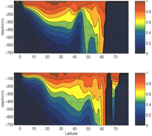
4.3.1 The modeled tracer distributions in the NADW . . . . 114
4.3.2 Normalized sensitivity . . . . 114
4.3.3 Propagation pathway and the associated timescale . . . . 116
4.3.4 Quantitative comparison: normalized sensitivities to the isopy-cnal mixing and thickness diffusion . . . . 122
4.4 Sensitivities of tracer properties in the lower subtropical thermocline . 126 4.5 Sum m ary . . . . 134
5 Constraining the North Atlantic Circulation with the Transient Tracer Observations 136 5.1 D ata error . . . . 140
5.2 Optimization of the CFC boundary conditions . . . . 143
5.2.1 Failed optimization over the entire North Atlantic . . . . 144
5.2.2 Optimization over the Atlantic between 4.50S and 39.50N . . 146
5.3 Optimization of the tritium boundary conditions . . . . 160
5.4 Sum m ary . . . . 172
6 Conclusions 173 6.1 Summary of the thesis . . . 173
6.2 D iscussion . . . .. 176
A The adjoint method 178 A.1 Description of the method . . . . 178
A.2 The descent method-quasi-Newton method . . . . 180
A .3 Procedure . . . . 181
A.4 An example of TMAC code construction . . . . 181
List of Figures
2-1 Evolution of the idealized tracer concentration with w = 10-6 M/s, , =
10-4 m 2/s, and A = 0. . . . . 40 2-2 Concentration difference between a decaying tracer (A = 3.836 x 10⁻¹² S-1)
and a stable tracer at year 6000 in a pipe flow with w = 10-6m/s and 10-rm2/s. Both tracers are forced by a unit step surface concentration. 41
2-3 Evolution of tracer distribution with different K (Mr2/s): 10-3 (left), 10-4 (middle), and 10-5 (right). w and A are 10-6 m/s and 0 s-1, respectively. Note the different depths at which the tracer penetrates in the steady states. 44 2-4 J as a function of w and , . The minimum point J=0 is indicated by the
star. Near the line w/ = 10-2, J is small (if J=0.1, the root-mean square
difference of model-data misfit will be 0.005). . . . . 46
2-5 Locations (denoted by stars) of model-produced "observations". The
back-ground is the evolution of the idealized tracer concentration in a pipe flow with w = 10-6 m/s and . = 10-4 m2/s. Contour intervals are 0.01 and
0.1 for concentration below 0.1 (dashed lines) and above 0.1 (solid lines),
respectively. . . . . 48
2-6 Distribution of the tracer concentration (black lines) given by the
inver-sion and the distribution of the idealized tracer concentration (red lines) in the pipe flow with w - 10-6 m/s and rn = 10-4 m2/s. Locations of
2-7 Constrained model (star) and observational (circle) tracer concentrations. Errorbars represent a white noise with standard deviation of 0.1. Notice that the model-data misfits fall within the errorbars. The "observations" in Fig. 2-5 are numbered from the top to the bottom and from early to late years. This numbering method leads to the chains of tracer concentration in the figure. . . . . 50 2-8 Locations (denoted by stars) of steady state "observations". The
back-ground is the steady state of the idealized tracer in a pipe flow with w = 10-6
m/s and K = 10-4 m2/s. Contour intervals are 0.01 and 0.1 for
concentra-tion below 0.1 (dashed lines) and above 0.1 (solid lines), respectively. . 51
2-9 Values of , and the surface tracer concentration during the inversion using
steady state "observations". . . . . 51
2-10 Locations (denoted by stars) of the decaying (A = 1.768 x 10⁻⁹) tracer "observations". The background is the tracer distribution in a pipe flow with
w = 10-6 M/s, r = 10-4 m2/s, forced by a unit step surface concentration.
Contour intervals are 0.01 and 0.1 for concentration below 0.1 (dashed lines) and above 0.1 (solid lines), respectively. . . . . 53
2-11 Evolution of the idealized tracer concentration in an oscillating pipe flow.
w = (10-6/V2)cos(ot) m/s, with a period T = 27r/o = 30 days. K is the
sam e as in Fig. 2-1. . . . . 55
2-12 Evolution of the idealized tracer concentration in an oscillating pipe flow. w = 10-6 + (10--6/V)cos(ot) m/s, with a period T = 27r/- = 2 years. r, is the sam e as in Fig. 2-1. . . . . 55 2-13 Evolution of the idealized tracer concentration in an oscillating pipe flow.
w = 10-6 + (10- 6
/10)cos(-t) m/s, with a period T = 27r/o- = 10 years. K
2-14 Evolution of the idealized tracer concentration in an oscillating pipe flow.
w = 10-6 + (10~6/10)cos(at) m/s, with a period T = 27r/o = 100 years.
The lower panel shows the tracer evolution in the first 300 years. Dashed lines represent tracer distribution in a steady pipe low with w = 10-6 m/s.
r, is the same as in Fig. 2-1. . . . . 57 2-15 Snapshots of the idealized tracer concentration at 360 m depth in the model,
from the beginning of year 1 to year 9. A unit step concentration in time is prescribed at each surface grid. The time of the panels increases from left to right, then from the top to the bottom. Land areas are shaded. .... 60 2-16 Climatological mixed-layer-depth (meter) in March from Monterey et al.
[1997]. The contour intervals are 50 m and 200 m for values below and
above 400 m, respectively. . . . . 61 2-17 Same as Fig. 2-15 but for 710 m depth. . . . . 62 2-18 The idealized tracer distributions at meridional sections 40.5'W (upper)
and 20.50W (lower) at the beginning of year 9 in the model. . . . . 64
2-19 Snapshot of the idealized tracer concentration at 1750 m depth at the
be-ginning of year 20 in the model. . . . . 65
2-20 Surface tracer concentrations (left panels) and the corresponding gradients of the cost function (right panels) at iteration 1 (upper panels), 5 (middle panels), and 20 (lower panels). The "observations" are uniform in space and perfect. . . . . 68
2-21 Value of the cost function and vertical background diffusivity during itera-tions. The "observations" are uniform in space and perfect. . . . . 69
2-22 Surface tracer concentrations at iteration 1 (upper) and iteration 20 (lower). The "observations" are uniform in space with a standard deviation of 0.33. 70 2-23 Sensitivity distribution of the cost function to surface tracer concentration.
The "observations" are perfect at cross sections 31.50N, 59.50N, 20.50W, and 40.50W. Note that sensitivity is concentrated along those cross sections. 71
3-1 The new model surface geometry with land areas dotted. Note that parts
of the northern and southern boundaries are open. . . . . 76 3-2 Estimates of atmospheric CFC-11 and CFC-12 concentrations (parts per
trillion) as a function of time and hemisphere, following Walker et al., [2000]. Values in the southern hemisphere are dashed. . . . . 76 3-3 Temporal distribution of tritium concentration in the North Atlantic surface
water, following Dreisigacker et al. [1978] and Doney et al. [1993]. .... 79
3-4 Estimated spatial coefficient of tritium concentration in the North Atlantic surface water; to obtain absolute tritium concentration, the value in this figure has to be multiplied by the temporal distribution in Fig. 3-3. . . 80 3-5 Map of tracer stations used in this study. Dots represent CFC-11/CFC-12
stations; triangles represent tritium stations. . . . . 80 3-6 Observational (upper) and modeled (lower) CFC-11 distributions nominally
along 20'W (WOCE A16N), July-Aug., 1988. Unit of CFC concentration is pmol/kg and hereafter. . . . . 84
3-7 Observational (upper) and modeled (lower) salinity distributions at the same section in Fig. 3-6. The salinity of the LSW is less than 34.94. . . . 84
3-8 Modeled CFC-11 (upper) and salinity (lower) distributions at 2200 m depth,
Jan. - Feb., 1998. Values of CFC-11 concentration higher than 1 pmol/kg and salinity lower than 34.95 are plotted out respectively to show the path-way of the LSW . . . . 85 3-9 Observational (left) and modeled (right) tracer distributions along a section
cross the Labrador Sea (WOCE AR07WD), June, 1993. . . . . 87 3-10 Observational (left) and modeled (right) CFC-11 (upper) and temperature
(lower) distributions along a section nominally 560
N (WOCE A01E), Sep., 1991. ... ... 89 3-11 Observational (left) and modeled (right) CFC-11 (upper), temperature
(mid-dle), and salinity (lower) distributions at 46'N (WOCE A02A ), Nov., 1994. Note the similar shape of the contours of CFC-11=3 pmol/kg, T=40C, and
3-12 Observational (left) and modeled (right) CFC-11 distributions nominally
along 240N (WOCE AR01), Jan. - Feb., 1998. The upper panels show the top 1000 m expanded. . . . . 92
3-13 Observational (left) and modeled (right) temperature (upper) and salinity
(lower) distributions at ~240N. . . . . 92
3-14 Observational (upper) and modeled (lower) CFC-1I distributions along 520W (WOCE A20), July-August, 1997. . . . . 94
3-15 Observed (upper) and modeled (lower) OT/Qy (0C/km) along WOCE A20
(-520W). The contour interval is 0.5 x10- 3 oC. . . . . 96
3-16 Observed (upper) and modeled (lower) oT/ox (0C/km) along WOCE AR01 (-240N). The contour interval is 0.5 x10- 3 oC. . . . . 96 3-17 The flow field at 2200 m depth in Feb. in the offline model. The maximal
velocity has a value of 5.7 cm/s. . . . . 97 3-18 Observed (upper) and modeled (lower ) tritium distributions (TU) along
the western Atlantic GEOSECS section, 1972. . . . . 99 3-19 Observed (left) and modeled (right) tritium distributions (TU) along
sec-tions nominally 20OW (Jul. - Aug., 1988), 460N (Nov., 1994), and 240N (A ug., 1981). . . . . 100 3-20 Observed (left) and modeled (right) 3He distributions (TU) along the section
nominally 460N, Nov., 1994. . . . . 101
4-1 Estimate of the atmospheric CFC-11/CFC-12 ratio as a function of time and hemisphere, following Walker et al., [2000]. Values in the southern hemisphere are dashed. . . . . 110
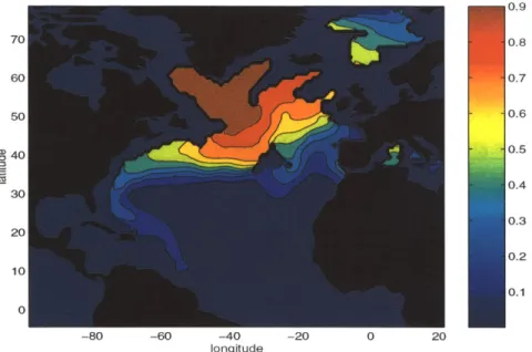
4-2 Distributions of the modeled 11 concentration(upper, pmol/kg),
CFC-11/CFC-12 ratio age (middle, year) and T+120 (lower, "C) at 2200 m, June
1980. The scales of the colorbars are chosen to let the southward spreading
4-3 Normalized sensitivities of the CFC-11 concentration in the NADW between depths 1335 - 2700 m and longitudes 80.5 - 60.5 oW at 30.50N, June 1980
to the meridional flow at depth 2200 m in February (a, (10-2 m/s)-1),
isopycnal mixing and thickness diffusion at depth 2200 m (b, (100 m2/s)-1),
surface piston velocity (c, (10-4 m/s)f), and background vertical mixing at depth 360 m (d, (10-5 m2/s) 1) at the end of 1977. . . . . 117
4-4 Normalized sensitivities of the CFC-11 concentration in the NADW between depths 1335 - 2700 m and longitudes 80.5 - 60.5 oW at 30.50N, June 1980
to the meridional flow ((10-2 m/s)-1 ) at 2200 m depth in February at the
end of year 1977 (a), 1973 (b), 1965 (c), and 1950 (d). . . . . 118
4-5 Normalized sensitivities of the CFC-11 concentration in the NADW between depths 1335 - 2700 m and longitudes 80.5 -60.5 oW at 30.50N, June 1980 to
the surface piston velocity in February ((10-4 m2/s)- 1) at the end of year 1977 (a), 1973 (b), 1965 (c), and 1950 (d). Note that values in the lower
panels are an order of magnitude larger than those in the upper ones. . . 119
4-6 Normalized sensitivities of the CFC-11/CFC-12 ratio age (upper) and r (lower) in the NADW between depths 1335 - 2700 m and longitudes 80.5
-60.5 'W at 30.50N, June 1980 to meridional flow ((10-2 m/s)-1 ) in February
at 2200 m depth at the end of year 1973 (left) and 1950 (right). Note that values in the lower panels are much larger than those in the upper ones. . 120 4-7 Normalized sensitivities of the CFC-11/CFC-12 ratio age in the NADW
between depths 1335 - 2700 m and longitudes 80.5 - 60.5 oW at 30.50N,
June 1980 to the surface piston velocity in February (left, (10-4 m2/s)- 1)
and T in the NADW to the surface value of r in February (right, ("C)1 ) at the end of 1950. ... ... 122 4-8 Normalized sensitivity of the CFC-11 concentration in the NADW between
depths 1335 - 2700 m and longitudes 80.5 - 60.5 OW at 30.50N, June 1980
to the isopycnal mixing and thickness diffusion ((100 m2/s)- 1) at 60.50W
4-9 Normalized sensitivities of the CFC-11 concentration (upper), CFC-11/CFC-12 ratio age (middle), and T (lower) in the NADW between depths 1335
-2700 m and longitudes 80.5 - 60.5 'W at 30.50N, June 1980 to the isopycnal
mixing and thickness diffusion ((100 m2/s)- 1) at 2200 m depth at the end
of year 1950. The left panels show the maximum values. . . . . 125
4-10 Distributions of the modeled 11 concentration (upper, pmol/kg),
CFC-11/CFC-12 ratio age (middle, year), and T+120 (lower, 'C) at 510 m depth, June 1980. ... ... 127
4-11 Modeled potential density distribution at 200W in March. . . . . 128
4-12 Modeled potential density distribution at the surface and the flow field at
510 m depth in March. . . . . 128
4-13 Normalized sensitivity of the CFC-11 concentration (upper), CFC-I/CFC-12 ratio age (middle), and r (lower) in the lower subtropical thermocline between depths 510 m and 710 m and longitudes 60.5 -20.5 oW at 30.50N,
June 1980 to the isopycnal mixing and thickness diffusion ((100 m2/s)- 1)
at 40.5'W at the end of year 1950. . . . . 131
4-14 Normalized sensitivity of the CFC-11 concentration in the lower subtropical thermocline between depths 510 m and 710 m and longitudes 60.5 - 20.5 oW
at 30.50N, June 1980 to the meridional flow ((10-2 m/s)-1) at 710 m depth in February at the end of year 1950. White lines represent the potential density and hereafter in this section. . . . . 132
4-15 Same as Fig. 4-14 with the eastern basin expanded. The white arrows are the modeled flow field at 710 m depth in February. . . . . 132
4-16 Normalized sensitivity of the CFC-11/CFC-12 ratio age in the lower sub-tropical thermocline between depths 510 m and 710 m and longitudes 60.5
- 20.5 OW at 30.50N to the meridional flow ((10-2 m/s)-1) at 710 m depth in February at the end of year 1950. . . . . 133
4-17 Normalized sensitivity of r in the lower subtropical thermocline between depths 510 m and 710 m and longitudes 60.5 - 20.5 oW at 30.50N to the
meridional flow ((10-2 m/s)-1) at 710 m depth in February at the end of year 1950. ... ... 133 5-1 Uncertainty profiles prescribed for different tracers in area 4.50S-39.50N,
99.50W-21.50E, 1990. Units of CFC and tritium are pmol/kg and TU,
respectively. . . . . 142
5-2 Distributions of the surface piston velocity in February at iterations 1 (left) and 4 (right). . . . . 145
5-3 Observational and modeled CFC-11 concentration (pmol/kg, and hearafter) along a section in the Labrador Sea (WOCE AR07W), June, 1993. The modeled convective mixing in the high latitudes is totally shut off. . . . . 146 5-4 The new model domain. Black dots represent CFC data stations. . . . . 147
5-5 The first estimate of the CFC-11 distribution at the northern boundary
(39.50N ) in 1994. . . . . 149
5-6 The optimal CFC-11 distribution at the northern boundary in 1994. White dots represent observational locations. . . . . 149
5-7 Comparison of the optimal (solid lines) and observational (dots) northern boundary CFC-11 concentrations in 1994. Errorbars represent the CFC-11 data error, dominated by the subgrid variability the model cannot resolve (See section 5.1 for details). . . . . 150 5-8 The constrained northern boundary CFC-11 concentrations (pmol/kg and
hereafter) in years 1981, 1982, ..., 1989 (left to right first) . . . . . 152
5-9 The constrained northern boundary CFC-11 concentrations in years 1990,
1991, ..., 1998 (left to right first). . . . . 153
5-10 The first guess of the piston velocity in February and the corresponding
difference between iterations 85 and 1 (85 - 1). . . . . 154
5-11 Differences of the initial CFC-11 concentrations at depth 3700 m between
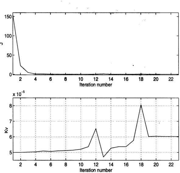
5-12 Value of the cost function during the optimization. . . . . 155 5-13 Distributions of observational (upper) and modeled CFC-11 concentrations
at iterations 1 (middle) and 85 (lower) along WOCE A20 (520W), July
-August, 1997. The contour intervals of white (below 0.5) and black lines (above 0.5) are 0.1 and 0.25, respectively. . . . . 156
5-14 Differences between the constrained and observational CFC-11 concentra-tions (model - data) along ~ 520W, WOCE A20. . . . . 158 5-15 Same as Figure 5-13 but for WOCE AR21 ( Repeated track of Oceanus
Cruise No. 202, ~200W ), July - August, 1993. . . . . 159 5-16 Stations (black dots) of the tritium data assimilated. . . . . 161 5-17 Distributions of observational (upper) and modeled tritium concentrations
at iterations 1 (middle) and 60 (lower) along the western Atlantic GEOSECS section, 1972. The contour intervals of white (below 1) and black lines (above 1) are 0.2 and 1, respectively. . . . . 163 5-18 Distributions of observational (upper) and modeled tritium concentrations
at iterations 1 (middle) and 60 (lower) along ~ 200W, July - August, 1988. The contour intervals of white (below 1) and black lines (above 1) are 0.2 and 0.5, respectively. . . . . 164
5-19 Tritium concentrations at the northern boundary (39.50N) in 1972 (upper), 1981 (middle), and 1992 (lower) at iterations 1 (left) and 60 (right). . . . 165 5-20 Cumulative observational tritium input from the ocean surface north of
39.50N (solid line) [Doney et al., 1993] and the constrained southward
tri-tium output across the northern boundary at 39.50N (dashed line) in the
North Atlantic. . . . . 167
5-21 Observational tritium water column inventory (x 103 TU81N-m) from TTO
5-22 The tritium budget in the region between 4.50S and 39.50N in the North
At-lantic: solid line, total oceanic tritium content from the constrained model; dashed line, total tritium input from the boundaries; dotted line, cumulative surface input from Doney et al. [1993]; dash-dot line, cumulative northern boundary input in the model. . . . . 168 5-23 Distributions of the optimal surface tritium concentration (TU) in 1964 and
the differences (TU) between iterations 60 and 1 (60 - 1). . . . . 170
5-24 Distributions of the optimal (upper) and observational (middle) surface tri-tium concentrations (TU) in 1981, and the differences (lower) of the surface tritium values in 1981 between iterations 60 and 1 (60 - 1). . . . . 171
List of Tables
2.1 Inverse solutions for w and r,, using transient stage "observations". .... 52
2.2 Inverse solutions for w and n,, using the decaying tracer "observations". . 54
2.3 The inverse solutions for nK. Note that the correct value should be 6.00 x
10- 5m 2/s. . . . . 66
3.1 CFC-11 and CFC-12 data sources. . . . . 81 3.2 Tritium and helium data sources except that from Khatiwala [2000]. . . . 81 3.3 Model-data misfits along WOCE sections. . . . . 102
5.1 Comparison of the studies about constraining the North Atlantic ocean cir-culation with the transient tracer data. . . . . 137
Chapter 1
Introduction
1.1
Transient tracers in the ocean
Transient tracers are a variety of man-made chemical species that have been intro-duced into the earth system, as a result of either industrial production or nuclear bomb tests. These anthropogenic tracers have made their way to the ocean through its surface. Because of their time-varying concentrations in the atmosphere, these man-made chemicals in the ocean are called transient tracers. Neither the oceanic distributions of these tracers nor their inputs are steady.
The most commonly studied transient tracers in oceanography are chlorofluorocar-bons (CFCs) such as CCl3F (CFC-11) and CCl2F2 (CFC-12), tritium, helium (3He),
and bomb radiocarbon ("C). CFCs are entirely man-made gases having been used
by refrigerators and manufacturing processes since the 1930s. Their concentrations
in the atmosphere continuously increased with time from the 1930s to the early 1990s [e.g., Walker et al., 2000]. The decomposition products of CFCs in the stratosphere cause the destruction of ozone [Anderson et al., 1991]. As a consequence of the Mon-treal Protocol, which limited the amount of CFCs emitted, the CFC increase rates dropped in the 1990s. Politicians and scientists continue working hard to decrease the amount of CFCs released into the atmosphere. CFCs enter the ocean through air-sea gas exchange.
water (HTO). The decay product of tritium is 3He. Oceanic 3He is composed of two parts: terrigenic 3He released from the ocean floor and tritiugenic 3He from tritium decay.
Major amounts of both tritium and C were produced as the result of atmospheric nuclear bomb tests in the early 1960s. Both isotopes were injected into the strato-sphere of the northern hemistrato-sphere, where the tritium atoms were quickly incorporated into H20 molecules and "C atoms into CO2 molecules. After being transferred to the
troposphere, bomb tritium and 14C followed quite different routes to the sea. Tritium
entered the ocean through direct precipitation, water vapor exchange between the at-mosphere and ocean, and river outflows [e.g., Weiss et al., 1980; Doney et al., 1993].
As the tritiated water molecules were quickly absorbed into raindrops or wet surfaces, tritium entered the ocean preferentially in the high-latitude northern hemisphere as a pulse in the 1960s. On the other hand, bomb 14C entered the ocean through gas
exchange of CO2 at the air-sea interface, and thereby was nearly uniformly spread in
the atmosphere before entering the sea [Nydal et al., 1983].
Once in the ocean, these chemicals are mixed and advected by the ocean circula-tion. A major motivation for studying the transient tracers in the ocean is to infer the ocean circulation, especially the exchange processes between the ocean surface and interior. These exchange processes are critical in redistributing not only heat and fresh water but also climatically important greenhouse gases such as CO2 globally.
Another objective for the study of the transient tracers in the ocean is to investigate the CO2 budget of the world ocean. Both CFCs and CO2 enter the ocean through
air-sea gas exchange. Because the biogeochemical carbon cycle is very complicated, we might hope that understanding the distributions of CFCs, which are chemically and biologically inert in the ocean, is a first step toward a better evaluation of the ocean's role in the global carbon cycle.
As described previously, the processes through which these tracers enter the ocean surface are very complex. To quantitatively infer ocean circulation from transient tracer distributions, reconstruction of the time-varying boundary conditions is essen-tial. This reconstruction requires extrapolation from a restricted amount of historical
data. For example, estimates of tritium concentration at the ocean surface are based on very sparse observations obtained by a few weather ships and research cruises, no-tably in the 1960s when the major amount of tritium entered the ocean [Dreisigacker et al., 1978]. Estimates of the surface CFC and CO2 fluxes are based on limited
knowledge about the complex air-sea gas exchange process. The relationship between the gas transfer velocity and wind speed is not yet totally understood [Wanninkhof,
1992]; the effects of boundary layer stability, turbulence and bubbles in the air-sea
tracer exchange are still uncertain. Inevitably, large uncertainties exist in the esti-mates of the transient tracer input functions. One focus of this study is interpreting the transient tracer distributions with uncertain input histories. There is another catalog of tracers that are released into the ocean under control, to investigate the circulation and dispersion in the ocean [Ledwell et al., 1993 etc.]. These tracers with accurately known input sources are not discussed here.
With great effort and big investments, a large amount of transient tracer data has been obtained from the world oceans. The Geochemical Ocean Sections Study
(GEOSECS) program in the early 1970s systematically sampled a number of natural
and anthropogenic tracers, such as tritium, 3He and 14
C, for the first time. In the
early 1980s, the Transient Tracers in the Ocean (TTO) program was carried out. The measurement of CFCs was introduced during the TTO North and Tropical At-lantic expeditions. Surveys of transient tracers continued with the South AtAt-lantic Ventilation Experiment (SAVE) in the late 1980s. Recently, more transient tracer observations were made along hydrographic sections of the World Ocean Circulation Experiment (WOCE). Despite these efforts, the transient tracer data are sparse when compared with measurements of traditional tracers, such as temperature and salinity
(T-S). This sparseness makes practical problems for the extraction of ocean
circula-tion informacircula-tion from the transient tracer data, that are very different from purely theoretical ones. Understanding the information content of transient tracers must ac-count for practical reality: the sparseness of data coverage and the large uncertainties in the transient tracer input histories.
A major application is to use these tracers as dyes to scrutinize the thermohaline
circulation, driven by the renewal of dense North Atlantic Deep Water (NADW) in the northern North Atlantic and by a smaller input of Antarctic Bottom Water (AABW) formed principally at the Weddell Sea [e.g., Schmitz, 1995; Haine et al.,
1998; Schlosser et al., 1991].
A synthesis of CFC observations is used to survey the large-scale circulation
path-ways and timescales for the spreading of NADW components, i.e, the Upper Labrador Sea Water (ULSW), the Classic Labrador Sea Water (CLSW), Iceland-Scotland Over-flow Water (ISOW), and Denmark Strait OverOver-flow Water (DSOW), by Smethie at el. [2000]. It is found that these water masses coincide with high CFC concentrations and have characteristic potential temperature, salinity and density. The pathways of these water masses are exhibited by CFC distributions, which are mapped from data of different cruises taken at different times. As Smethie et al. [2000] point out, a problem is presented when using transient tracers: their inputs vary with time and their distributions are not in steady states. To obtain the basin-scale distribution pattern from transient tracer data, corrections must be made to normalize concentra-tions sampled at different times. This has been done by using the CFC-11/CFC-12 ratio.
It is generally assumed that the CFC-11/CFC-12 ratio is conserved once a water parcel leaves the surface. This assumption is true if mixing is negligible or tagged water mixes only with free water. Based on this assumption, the
CFC-11/CFC-12 ratio age is derived according to the atmospheric CFC-CFC-11/CFC-12 ratio,
which increased steadily with time until the late 1970s. First, the CFC concentrations in sea water are converted to the corresponding dry air atmospheric mixing ratios, using Henry's law [e.g., Warner et al., 1985]. Here it is assumed that the potential temperature and salinity in a water mass are conserved. The dry air mixing ratio of
CFC-11/CFC-12 is then compared to the appropriate historical atmospheric ratio of CFC-11/CFC-12 to determine the time when the water parcel was last at the ocean
surface [Doney et al., 1997]. Smethie et al. [2000] use the CFC-11/CFC-12 ratio age to infer the timescales for the spreading of NADW components. Because there are
recirculation, mixing, and entrainment of CFC-tagged water in both upper and deep ocean, inferences based on the CFC age are biased.
Smethie et al. [2000] assume the oceanic CFC concentrations at a specific obser-vational location change at the same rates as the atmospheric CFCs at the year when the observed water parcel left its source region. Using this assumption, Smethie et al. [2000] normalize the CFC concentrations sampled at different years to the same year. Large errors are introduced in the normalization and mapping processes to obtain the basin-scale distributions of CFCs. Inferences from the spatial distributions of CFCs have large uncertainties.
A review of the application of transient tracers as well as other natural tracers
in studies of the Weddell Sea is given by Schlosser et al. [1991]. Tritium and CFC concentrations are used to qualitatively interpret channels where newly formed young waters leave the shelves of the Weddell Sea and flow down the continental slope into the deep basin. The CFC-11/CFC-12 ratio together with CFC-11/tritium ratio is used to estimate the transit times of young waters, because the CFC-11/tritium ratio increased monotonically between 1975 - 1987 when the CFC-11/CFC-12 ratio was
nearly constant. Again, the effect of mixing among CFC-enriched waters is neglected. Schlosser et al. [1991] also discuss the use of steady tracers 180 and Helium isotopes to distinguish deep waters and their pathways from different surface source regions, because the concentrations of these steady tracers are different in glacial meltwater and seawater.
The export of AABW from the Weddell Sea into the southwest Indian Ocean is estimated by Haine et al. [1998], using CFC data. The routes of AABW leaving the Weddell Sea have been described by Mantyla et al. [1995], according to traditional hydrographic structures, i.e., distributions of potential density anomaly, potential temperature, salinity, dissolved oxygen and silicate. In Haine et al. [1998], the transient tracer fields confirm the pathway of AABW established by the analysis of steady tracer distributions. An along-stream advection and cross-stream mixing model is established by Haine et al. [1998]. Using this simple kinematic model and assuming that the surrounding water of AABW is CFC-free, Haine et al. [1998]
estimate the outflow speed and mixing rates for the AABW transport.
The pathways of water between the Pacific and Indian oceans in the Indonesian seas are investigated by Gordon and Fine [1996]. T-S and CFC-11 distributions at different locations of Indonesian Sea are combined together to infer the pathways of the Indonesian through-flow (ITF). Water with similar T-S and CFC properties is attributed to the same origin. Gordon and Fine [1996] conclude that the ITF is dominated by two components: one of low-salinity, well ventilated North Pacific water through the upper thermocline of the Makassar Strait, and the other of more saline
South Pacific water through the lower thermocline of the eastern Indonesian seas. There are published papers about studies of deep water formation processes at the Ross Sea [Trumbore et al., 1991], Red Sea [ Mecking et al., 1999], and Arctic Ocean [Anderson et al., 1999], using transient tracer observations. But we should notice that, in the oceanographic literature (including some of the studies mentioned above), formations and pathways of the upper ocean central waters (e.g., 180 mode water), intermediate waters (e.g., Antarctic Intermediate Water), deep waters (e.g.,
NADW), and bottom waters ( e.g., AABW), have been successfully explored and
depicted by employing approximately steady tracers (e.g., T-S, oxygen, silicate). See Pickard and Emery [1990] for a summary. The roles of both transient and steady tracers need further examination.
Besides qualitative interpretations of flow paths, quantitative inferences about water mass formation rates, mixing rates and ventilation timescales are made from the transient tracer data. Smethie et al. [2001] estimate the formation rates of the
NADW components, using CFC observations and the equation,
I
=E RCst.
(1.1)Here I is the total CFC-11 inventory, R is the rate of water mass formation, C. is the CFC-11 concentration in the source water as a function of time, and 6t is the time step. First, vertical profiles of CFC-11 are segmented into components of
water column inventory. The water column inventories are normalized to year 1990 and mapped, using the method in Smethie et al. [2000], which has been described previously. The total inventory I is obtained by integrating the map of the water column inventory. The summation is carried out over the time period of CFC input, 1945 - 1990. C, is estimated from the atmospheric history of CFC-11 concentration,
the CFC-11 solubility, and the saturation at the source region of a specific water mass. The saturation is assumed to vary among different source regions but remain constant with time. The formation rate R of each water mass is also assumed to be constant in time.
During these processes to obtain the formation rate R, a large error is introduced
by constructing the map of CFC-11 water column inventory from sparse data. There
are errors in the source water concentration C8, arising from the uncertainty in the
saturation of CFC-11 in the source water, uncertainty in the T-S of the source water which determine the CFC solubility, and uncertainty in the atmospheric CFC history. The total NADW rate given by Smethie et al. [2001] is 17 Sv with 30% uncertainty, as compared to 14 Sv estimated from hydrography and current measurements (see Schmitz, 1995 for a review).
Jenkins [1991] calculates the isopycnal eddy diffusivity in the Sargasso Sea, using the tritium-3He age equation
=KV2 T-V-Vr+++K
+ -VT. (1.2)
at 0
Here T is the tritium-3
He age, K is the isopycnal diffusivity, V is the isopycnal velocity,
( is the sum of tritium and 3He, and 0 is tritium. The tritium-3
He age [Clarke et al.,
1976] is defined as
T = 17.93 In (3H.He (1.3)
3H
Jenkins [1991] estimates the spatial and temporal derivatives of T, (, and 0 directly
from observations. The isopycnal diffusivity is calculated as
+V -VT -1
K= T (1.4)
(V2T±(V+ ) -VT)(
Generally, the transient tracer observations are made at different times in different areas. The transient tracer data are sparse in most of the ocean regions. Therefore, the spatial and temporal derivatives of T, (, or 0 obtained directly from observations
are inaccurate.
A common approach to infer mixing rates is by fitting data to simple models [e.g.,
Haine et al. 1998]. Using observed tritium profiles and a one-dimensional advection-diffusion model, Kelley et al. [1999] estimate the vertical diffusivity , in the upper
subtropical North Pacific and give K, = (1.5 t 0.7) x 10-5m2
/s.
By fitting aone-dimensional advection-diffusion model to CFC data in the upper North Pacific at
500N, Matear et al. [1997] obtain s, = (4 i 0.1) x 10-5m2
/s.
As the inferences fromthe transient tracer data are based on very simple models and assumptions, those inferences should be regarded as rough first-order approximations which need to be improved using more realistic models [ Schlosser et al., 1991].
Quantitative inferences of timescales of ocean circulation from the transient tracer data are based on tracer ages. The derived tracer ages are treated as proxies for the ideal age, defined as the elapsed time since a water parcel was last exposed to the atmosphere [e.g., Doney et al., 1997]. Intuitively, it is believed that tracer age simplifies interpretation of the transient tracer distributions mainly due to its simple surface boundary condition, which is zero. On the other hand, as Wunsch [2002] points out, the simplification of the boundary condition of the tracer age is at the sacrifice of losing the linearity of the governing equation, in the geophysical fluid system. Analytical solutions show that the expression of the tracer age is more complicated than that of the tracer concentration. Interpretation of the tracer age is very difficult.
Holzer and Hall [2000] argue that a water mass comprises a distribution of times [e.g., Hall and Plumb, 1994] since it made contact with the surface, via a multiplicity of pathways. The mean age is the first moment of the transit time probability density function (pdf), i.e., the mean transit time. The ideal age converges to the mean age when it reaches a steady state [e.g., Holzer and Hall, 2000; Haine and Hall, 2001]. Any tracer measurement, steady or transient, provides integrated information about
transit times. The water mass composition of steady tracers includes a distribution of transit times for tracer originating from each surface source point [Haine and Hall, 2001]. On the other hand, the transient tracer ages have no simple relation to the mean transit time, because not all pathways from the surface have been sampled by the transient tracers. For example, a CFC sample contains no information about transit times exceeding 80 years. In the presence of turbulent mixing, the transient tracer ages are biased estimates of the true ocean ventilation age.
The pdf of transit times can be represented as a boundary Green function [e.g., Holzer and Hall, 2000; Haine and Hall, 2001]
G - VG - V - (KVG) = 0, (1.5)
at U
with the concentration boundary G = 6(t - t') defined in a region Q of the ocean surface. Here U' and K represent the flow field and mixing tensor, respectively. The boundary Green functions serve as diagnostics in a numerical model. No inference of boundary Green function has been obtained from transient tracer observations. Because the boundary Green function itself depends on the flow field and mixing rates, improvements of the model circulation are fundamentally important for us to understand the transport processes and their timescales.
There is a growing literature about the use of transient tracers to improve model performances. Commonly, the transient tracer observations are compared with model predictions to evaluate ocean models [e.g., Craig et al., 1998; England, 1995; Sarmiento,
1983]. A comprehensive review of using chemical tracers in ocean models is given by
England and Maier-Reimer [2001]. In these papers, it is reported that the model predictions and observations agree reasonably well. Noticeable differences, however, remain. Comparisons between model results and observations show disagreements on issues such as the deep water formation in the high latitudes. For example, England and Hirst [1997] find excessive downward penetration of CFC-11 in the high latitude Southern Ocean, which is related to excessive vertical convection at these latitudes. In the North Atlantic, most model simulations [e.g., England and Hirst, 1997; Craig
et al., 1998] capture only a single core, corresponding to the upper NADW. The lack of a deeper core is due to the absence of Overflow Water (OW) in the models [e.g., England, 1998]. As Craig et al. [1998] point out, problems with deep water mass for-mation lead to the model-data disagreements in CFC pathways downstream. Model-data misfits of tracer distributions in the Antarctic Intermediate Water (AAIW) are also reported by Craig et al. [1998]. Modeled CFC penetration in the AAIW is too weak, associated with erroneous water mass structure; the modeled AAIW is too warm and its volume is too small. In general, model-data discrepancies of transient tracer fields appear in regions where the modeled and observed water mass structures are different.
One technique to nudge modeled T-S fields towards observations is restoring three-dimensional T-S but not transient tracer fields in the model. This restoring changes the evolution dynamics of T-S. Because the governing physics of T-S and transient tracers are no longer the same after restoring, their signatures of model-data misfits are different sometimes; the modeled T-S might be in good agreement with the ob-servations while the transient tracers might not. The restoring technique is useful for forward simulations. When we want to evaluate and improve the model physics and thus the model performance, we should, however, let the model physics play their roles freely without any purposeful forcing.
In a model of the real ocean, both transient and steady tracers are governed by the same physics. All characteristic properties of a water mass, the transient tracer concentrations as well as its T-S, will be imprinted along its trajectory. A water mass can be identified by its traditional hydrographic structure, such as T-S, oxygen and silicate. For example, Talley et al. [1982] successfully exhibit the pathway of the newly ventilated Labrador Sea Water (LSW) from salinity distribution. T-S can also be used to locate rapid mixing processes where vertical homogeneity is present. The under-saturation associated with deep convection can be demonstrated by oxygen field. A systematic investigation of the roles of both transient and steady tracers in helping us to evaluate model performances is needed.
transient tracer observations, that is, incorporating the transient tracer observations as constraints on an ocean circulation model. This is another approach to extract information from sparse transient tracer data. The pioneering work of Memery and Wunsch [1990], using a geostrophic coarse box model and a Green function approach, shows that uncertainty in the transient tracer boundary conditions and sparse data coverage greatly weaken the ability of tritium to constrain the model.
Almost 10 years later, Gray and Haine [2001] combined a North Atlantic ocean general circulation model (OGCM) with CFC observations. They give 23 smeared im-pulsive sources on the North Atlantic surface and solve for the corresponding bound-ary Green function components. Given that the CFC concentration is zero at the initial time, the CFC concentration at location r and time t is represented by these Green function components
C(r, t) =
E
G(r, t; i, to)BN(i, to)dto. (1-6)Here G(r, t; i, to) represents the boundary Green function at location r and time t, forced by the ith smeared impulse at time to; BN(i, to) is the CFC surface flux at the location of the ith impulse at time to. In Gray and Haine [2001], the ocean circulation is assumed to be steady. This assumption leads to G(r, t; i, to) = G(r, t-to; i, 0), which greatly reduces the computational expense. The CFC surface flux BN is constrained
by minimizing model-data differences of CFC-11 and CFC-12. The boundary Green
function components are stored annually at the end of August and observations are adjusted to late summer values. The result of Gray and Haine [2001] shows that after optimization of the surface fluxes, the model and data are marginally consistent.
Some issues arise in the above application of the Green function theory. When a tracer distribution is represented in terms of Green function components, they should include all components due to impulse sources at all points and all times. When the impulses are smeared and the integrations are discretized as summations over large steps, uncertainties are introduced. Within the surface region of each smeared im-pulse, the CFC flux BN has to be constant in space. Because the gas-exchange rates
of CFCs depend on wind speed, for which the spatial variability is large, the assump-tion of constant CFC flux in space within a large-scale region certainly introduces errors. As the sources are all located on the ocean surface, lateral fluxes of CFCs are totally ignored in Gray and Haine [2001]. An inverse study that allows more realistic transient tracer boundary conditions is needed.
1.2
The transient tracer problem
While the oceanic transient tracer data are now common, there are difficulties with their quantitative use. As Wunsch [1988] points out, direct inferences of ocean circu-lation parameters from the transient data are not straightforward. Considering any passive tracer C, its concentration satisfies an equation like
DC
+u -VC - V - (KVC = -AC+ S, (1.7)
at
where S represents sinks/sources, A is a decay constant, U' is velocity, and K is the mixing tensor. Inferences from transient tracer distributions require our knowledge about the initial-boundary conditions and the derivatives of C. There inevitably exist large degree of uncertainties in the time history of the transient tracer boundary conditions. Given the difficulties and expense of collecting transient tracer data, it is impractical to obtain accurate temporal and spatial derivatives of C from the sparsely distributed transient tracer data.
These difficulties can be overcome by the use of approximately steady tracers (simply called steady tracers hereafter). If we want to infer the first order large-scale mean ocean circulation from steady tracer observations, we can combine measure-ments made at similar climatological conditions together to yield a complete spatial picture, in a way that is impossible with the transient tracers [Wunsch, 1987]. In addition, the traditional steady tracer observations are far more abundant than the transient observations.
and fresh water transports in the ocean are made from measurements of steady trac-ers, such as T-S, oxygen, silica and phosphate [e.g., Ganachaud and Wunsch, 2000]. With OGCMs, estimation of the daily-evolving large-scale ocean circulation is made possible through a combination of traditional hydrography, expendable bathyther-mograph (XBT), surface drifters and deep floats, altimetric data sets and dynamics [Stammer et al., 2002]. The existence of these competing data sets leads to a ques-tion: how much additional information about the ocean circulation can the transient tracers provide us, given our current knowledge?
Incorporation of real transient tracer data in a model requires a long-term trans-port integration, because the transient tracer distributions at observational times depend on their previous histories. The large degree of uncertainty in the transient tracer input histories is one of the major difficulties in obtaining quantitative infor-mation about ocean circulation from the transient tracer data. For some tracers, such as helium, it is very difficult to quantify the mantle sources. Separating natural and bomb-produced distributions of 1 4C is still a challenge [Toggweiler et al., 1989].
Practically, whether the inherent temporal variabilities of the sparse transient tracer data can be used to provide unique information about ocean circulation, or on the contrary, the complexity of the temporal variabilities actually undermines the system-atic and quantitative inferences, is still unknown. Efficiently constraining the surface and lateral boundary conditions is a prerequisite to evaluate the extent to which the transient tracer observations can constrain the ocean circulation, and thereby enhance our present estimation of the ocean state. In addition, the long term integration re-quirement puts a great computational burden on the assimilation of transient tracer data into a comprehensive OGCM.
1.3
Objectives
This thesis is directed at understanding, evaluating, and using the information content of the transient tracers. Specifically, this study will explore the potential capabilities of both transient and steady tracers in the contexts of model evaluation and data
assimilation, and quantitatively access the extent to which the current transient tracer data can constrain the large-scale ocean circulation properties. The results of this study can provide useful information for designing future observational strategies.
Our area of interest here is the North Atlantic, because its circulation contains a range of physical processes, including deep water formation. It is also one of the regions best covered by transient tracer observations. This study investigates not only the roles of both transient and steady tracers in tracking the formation of the NADW and its pathway in a forward model, but also analyzes and compares amplitudes, propagation timescales and pathways of the sensitivities of transient and steady tracer properties in an adjoint model (see Appendix A). In doing so, we try to understand the information content of transient tracers relative to steady tracers.
Because the transient tracer data are sparse, a direct combination of a numerical model with the data is one of the major techniques to quantitatively use the transient tracer data. There are many published papers about assimilation of T-S observations in OGCMs [e.g, Stammer et al, 2002; Yu et al., 1996; Schlitzer, 1993], yet studies of assimilation of transient tracer data in an OGCM are few. A study is needed to explore whether the transient tracer data can provide additional information, using realistic transient tracer boundary conditions. A major objective for the study of transient tracers in the ocean is the possibility that they can improve the estimates of surface CO2 flux. Therefore, investigation of the extent to which the gas exchange
rates at the air-sea interface can be constrained by CFC observations is important. As recommended by M6mery and Wunsch [1990], this study continues to explore the capability of the present transient tracer observations to constrain ocean circu-lation properties in an OGCM. Unlike the work of Gray and Haine [2001], in which assumptions of constant inter-annual saturation rate in the mixed layer and smeared impulse surface sources in space are made, we use realistic CFC surface fluxes at each model-grid point with temporally and spatially varying saturation in the mixed layer. Compared to the model used by Gray and Haine [2001], our model has a higher resolution and allows tracer fluxes across open boundaries. More important, in this study, we seek to evaluate the extent to which the transient tracer data can constrain
![Figure 2-16: Climatological mixed-layer-depth (meter) [1997]. The contour intervals are 50 m and 200 m for respectively.](https://thumb-eu.123doks.com/thumbv2/123doknet/14460174.520344/61.918.174.732.270.805/figure-climatological-mixed-layer-depth-contour-intervals-respectively.webp)