The development of an acoustic levitation test facility for cloud physics research

by Victor D. Lupi

S.B., Massachusetts Institute of Technology (1988)

SUBMITED TO THE DEPARTMENT OF AERONAUTICS AND ASTRONAUTICS IN PARTIAL FULFILLMENT OF THE REQUIREMENTS FOR THE

DEGREE OF

MASTER OF SCIENCE IN AERONAUTICS AND ASTRONAUTICS at the

MASSACHUJSETTS INSTITUTE OF TECHNOLOGY (December 1989)

© Massachusetts Institute of Technology

Signature of Author

Certified by

1989

Department of Aeronautics an Astronautics December 22, 1989

Associate Professor R. John Hansman Thesis Supervisor, Department of Aeronautics and Astronautics

Accepted by 'ASSACHUSE1TS INSTITUTE KASSACHUSETTS INSTITUTE OF TECHNnl OGY FEB 2 1990 LIBRAREM' ARCHIVES

PIofessor Harold Y. Wachman Chairman, Ddartment Graduate Committee

by

Victor D. Lupi

Submitted to the Department of Aeronautics and Astronautics on December 22, 1989 in partial fulfillment of the requirements for the degree of

Master of Science in Aeronautics and Astronautics.

Abstract

An Acoustic Levitation Test Facility appropriate to cloud physics laboratory

experiments has been developed. The facility utilizes acoustic standing waves to accurately control the location of single or multiple hydrometeors (water droplets or ice crystals) without direct physical contact. This unique capability allows the facilities to complement existing experimental methods, such as free fall chambers and vertical wind tunnels, where the transient nature of the testing makes carefully controlled experiments difficult. In addition, the small size of the acoustic levitator allows easy access of diagnostics to the test region.

Two separate levitation facilities have been built. In the Vertical Facility, a vertically oriented acoustic levitator utilizes a strong acoustic field to support objects against the force of gravity. The surrounding medium in which the suspended object is held is essentially

motionless. In the Ventilated Facility, a small vertical wind tunnel provides the levitating force on the suspended object. This force, arising from aerodynamic drag on the object, opposes the gravitational force on it. In this facility, a horizontally oriented acoustic field is used to stabilize the suspended object within the flow field of the wind tunnel. The motion of the surrounding medium is approximately that of the terminal velocity of the suspended sample.

The theory of acoustic levitation is presented in detail. Predictions are made concerning the performance of the levitation device for solid and liquid samples. For solid spheres, the levitating force diminishes as the diameter approaches the acoustic wavelength. For liquid samples, the deformation of the droplet under the acoustic forces is considered. The predictions are compared with experimental results to validate the theory. Solid samples as large as 9 mm in diameter and liquid samples as large as 4 mm in diameter were levitated in the Vertical Facility.

The effects of the acoustic field on molecular diffusion phenomena was addressed. The evaporation rates of droplets suspended in the acoustic field were compared with the

evaporation rates of droplets suspended from a fine glass thread. It was determined that the acoustic field does not significantly affect water vapor diffusion.

The ability to study phase change phenomena in both facilities was demonstrated. Droplets were frozen while levitated in the Vertical Facility. The frozen droplet remained stable in the acoustic field. In the Ventilated Facility, the freezing of droplets in free fall was

simulated. The frozen droplets remained stable in the test section until shape asymmetry effects, caused primarily by nonuniform ice accretion, became significant.

Thesis Supervisor: Professor R. John Hansman

Acknowledgements

First and foremost, I would like to thank Prof. RJ. Hansman for his seemingly

limitless patience and perseverance, and for his advice and inspiration during the many times it was needed. I would also like to thank Paul Bauer and Al Shaw for their technical expertise and willingness to help tackle the practical issues associated with this thesis. In addition, I would like to express my appreciation to my parents, Nino and Lydia, who have continually supported my efforts. Thanks, also, to Debi Jones, for her knowledge of word processing systems and attention to detail. Finally, thanks to the students and dreamers of the

Aeronautical Systems Lab that I have come to know over the past two years. This work was supported by the National Science Foundation.

Table of Contents

Nomenclature 4

1. Introduction 6

1.1 Background 6

1.2 Unique Features of the Acoustic Levitation Test Facility 7

1.3 Motivation for Developing Two Facilities 9

1.4 Outline of the Thesis 11

2. Theory of Acoustic Levitation 12

2.1 Introduction 12

2.2 Levitation of Solid Objects 12

2.2.1 Net Acoustic Force on Rigid Spheres in a Planar Standing Wave 13 2.2.1.1 Problem Description and Boundary Conditions 14 2.2.1.2 General Solution of Wave Equation 18 2.2.1.3 Application of the Boundary Conditions 20 2.2.1.4 Determination of Pressure Variation Over Surface of Sphere 22 2.2.1.5 Net Effect of Acoustic Pressure Distribution on Sphere 24 2.2.1.6 Levitation Limit for Large Spheres 27 2.2.2 Stability of Spheres in Acoustic Levitation Environment 30

2.2.2.1 Gravity-Free Environment 30

2.2.2.2 Levitation Against Gravity 31

2.3 Levitation of Liquid Droplets 34

2.3.1 Distortion of Droplet Shape from Spherical 35

2.3.1.1 Mathematical Model 35

2.3.1.2 Predictions Based on Mathematical Model 41 2.3.2 Droplet Oscillations in the Acoustic Field 44

3. Development of the Acoustic Levitation Hardware 49

3.1 Principle of Operation 49

3.2 Design of Driver 49

3.2.1 Choice of Operating Frequency 51

3.2.2 Design of Driver Elements 51

3.2.2.1 Resonator 53

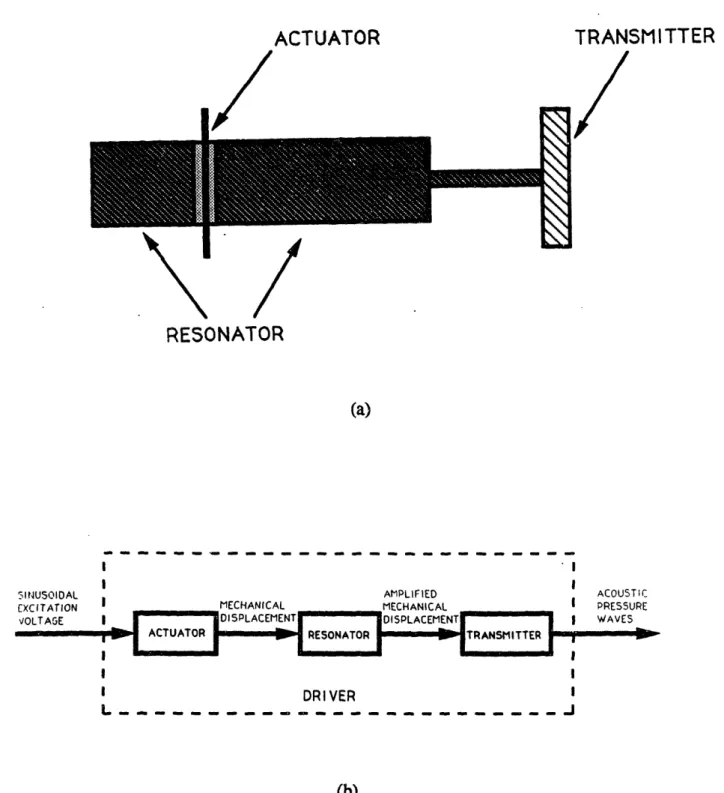
3.2.2.2 Actuator 54

3.2.2.3 Transmitter 56

3.2.3 Description of Driver Hardware 58

3.2.4 Driver Resonance Tracking 63

3.3 Reflector Assembly 67

4. Description of Facilities 72

4.1 Overview 72

4.2 Vertical Facility 72

4.2.1 Description of the Vertical Facility 72

4.2.2 Temperature Compensation System 76

4.3 Ventilated Facility 81

4.3.1 Principle of Operation 81

4.3.2.1 Wind Tunnel 84 4.3.2.2 Test Section and Acoustic Levitator Hardware 89

4.3.2.3 Design of Droplet Injector 92

4.4 Diagnostics and Data Acquisition 98

5. Validation of the Facilities 99

5, 1 Effect of the Acoustic Field on Ambient Conditions in the Test Section 99 5.1.1 Temperature Gradients in the Test Section 99

5.1.2 Molecular Diffusion Processes 101

5.2 Effect of the Acoustic Field on Levitated Hydrometeors 104

5.2.1 Solid Samples 104

5.2.2 Liquid Samples 106

5.2.2.1 Droplet Shape Distortions in the Vertical Facility 106 5.2.2.2 Capture Range Enhancement in the Ventilated Facility 111

5.2.3 Phase Change Phenomena 114

6. Conclusion and Recommendations 119

6.1 Summary of Results 119

6.2 Recmmendations for Future Development 120

6.3 Potential Experiments for the Facilities 121

Appendix A - Details of Acoustic Levitator Hardware 123

Appendix B Details of Resonance Tracking System 128

Appendix C - Details of Refrigeration System

133

Nomenclature

a radius of a spherical object (m) a radius of transmitting plate (m)

A amplitude of velocity potential of acoustic field (m2/sec)

An, An arbitrary constants associated with solution of wave equation (m2/sec) c speed of wave propagation in an acoustic medium (m/sec)

Cn coefficients of the harmonic expansion of the deformed droplet shape (-) d separation distance between driver and reflector (m)

dI, d2 shape parameters of resonating structure (m)

D, diffusivity of air (m2/sec)

_ modulus of elasticity of resonating structure (Nt/m2) E time-averaged acoustic energy density (J/m3)

E rin l minimum acoustic energy density required for levitation (J/m3) E normalized acoustic energy density (-)

f operating frequency of the acoustic levitator (Hz) fn spherical wave function (-)

Fn, Gn arbitrary constants associated with solution of wave equation (-) g acceleration due to gravity (m/sec2)

h distance from nodal plane to center of spherical object (m) h thickness of transmitting plate (m)

i index

j

(-)

j index (-)

J curvature of droplet expressed in terms of deformation harmonics (-) k acoustic wave number (m-l)

k index (-)

L length of resonating structure (m)

m index (-)

n number of nodal planes in acoustic standing wave (-)

n index (-)

NBO Bond number (-)

NAC nondimensional acoustic parameter (-) p pressure in an acoustic medium (Nt/m2₎

Po ambient atmospheric pressure in the absence of an acoustic field (Nt/m2) Pi_ internal pressure within a water droplet (Nt/m2)

P time-averaged acoustic force on an object in acoustic field (Nt) Pn Legendre polynromial (-)

q magnitude of the velocity in an acoustic medium (m/sec)

qn coefficients of harmonic expansion of pressure distribution around droplet (-) ro radius at top of deformed droplet (m)

R gas constant for air (J/kg-K)

R1,R2 principal radii of curvature of deformed droplet (m)

Rn, Sn arbitrary constants associated with solution of wave equation (-) S.4 ambient saturation ratio (-)

Sn spherical surface harmonic (-)

t time (sec)

-T nondimensionalized acoustic force on an object (-) T ambient temperature (K)

u longitudinal displacement associated with axial vibrations of a rod (m) U nondimensionalized pressure distribution over an object (-)

V volume of a droplet (m3)

V1,V2 displacement amplitudes at either end of resonating structure (m)

x dummy variable

z vertical coordinate of center of a droplet in a planar acoustic standing wave (m) zW, equilibrium location of droplet in acoustic field (m)

specific heat ratio for air (-)

p ;essure deviation from ambient due to acoustic field (Nt/m2) 8z displacement of an object within acoustic field (m)

perturbation of an object from equilibrium within an acoustic standing wave (m) acousc wavelength (m)

Xij modal eigenvalue of axisymmetric vibration of transmitting plate (-) p. spherical coordinate (-)

v Poisson's ratio of transmitting plate (-) p density of resonating structure (kg/m3) p density of transmitting plate (kg/m3) P0 density of air (kg/n3)

Pi density of object suspended in acoustic field (kg/m3) Psal ambient saturation vapor density (kg/m3)

Psat,a saturation vapor density at surface of droplet (kg/m3) a surface tension of a droplet (J/m2)

Oh, spherical wave function (-)

· velocity potential of acoustic field (m2/sec) (1_{I veloci:y potential of incident wave (m}2_/sec)

Vn spherical wave function (-)

X operating frequency of driver (rad/sec)

cor fundamental modal frequency of shape oscillation of a droplet (rad/sec)

xoWC

'Oi modal frequencies of axisynmetric vibration of transmitting plate (rad/sec)

AA A

r, 0, 6 unit vectors in spherical coordinates (-)

Chapter 1

Introduction

1.1 Background

The study of cloud physics is essential to many areas of research. In the field of meteorology, hydrometeor microphysics and droplet dynamics play an important role. The formation of clouds, the initiation of precipitation, the formation of ice, and the electrification of the atmosphere are all based on microphysical phenomena. Aviation technology is also driven by an understanding of these phenomena. For example, understanding and preventing the formation on ice on aerodynamic surfaces requires knowledge of the physical conditions that initiate the icing process. Clearly, the ability to simulate various conditions in the laboratory would serve to advance this technology. The study of the interaction of radar signals with the atmosphere is also a rich topic. In particular, much interest lies in the change in radar attenuation and scattering by the atmosphere when the ambient water vapor undergoes a phase change. Many other topics that rely on knowledge of cloud microphysics exist. Studying these phenomena in the laboratory is difficult, however, as many of these processes occur over long time intervals and have appreciable effects only over large volumes of the atmosphere. For example, free fall chambers are limited by their vertical dimension. The observation time is fixed by the time it takes for the test sample to fall through the test section, making it impossible to study long term effects on hydrometeors. Vertical wind tunnels attempt to solve this problem, with limited success. This is primarily due to the lack of in-stream and lateral stability of the suspended sample in the test section. The lack of these forces cause the samples to either hit the walls of the test section or be carried downstream by the flow. It is therefore desirable to augment the existing set of laboratory apparatus with a facility better capable of maintaining the stability of the hydrometeor while accurately simulating the ambient environment.

To this end, a set of acoustic levitation test facilities appropriate to cloud physics laboratory experiments have been developed. The facilities utilize acoustic standing waves to accurately control the location of single or multiple hydrometeors (water droplets or ice crystals) without direct physical contact This unique capability allows the facilities to

complement the existing experimental methods mentioned above, where the transient nature of the testing makes carefully controlled experiments difficult. In addition, the small size of the acoustic levitator allows easy access of diagnostics to the test region.

1.2 Unique Features of the Acoustic Levitation Test Facility

The concept of levitating small particles by acoustic radiation pressure was proposed as early as 1934 by King [1]. However, it was not until the 1970's that acoustic drivers were sufficiently powerful to allow practical application of acoustic levitators. Currently, levitators are primarily used for containerless materials processing and space shuttle experiments [2][3]. In a typical levitator, shown schematically in Fig. I-1, an acoustic standing wave is generated between a transmitter and a reflector separated by an integral number of half wavelengths. The rarticle is supported against gravity by the pressure forces and tends towards a stable

equilibrium position in the vicinity of the acoustic nodal planes. A curved reflector surface focuses the acoustic field, creating secondary pressure forces which position the particle to a point within the nodal plane that lies along the axis of the device. Thus, both vertical and horizontal stability is achieved with a single device.

Acoustic levitation holds several unique advantages over conventional experimental techniques (e.g., vertical wind tunnels, free fall testing, mechanical suspension or in situ measurement). There are, however, limitations of the acoustic technique as a cloud physics research tool, which are discussed in detail in Chapter 2.

The principal advantage of the acoustic levitation technique is the ability to support particles in a precise manner for indefinite periods of time. The stability in position control for a typical vertical levitator is on the order of one droplet diameter or less. This is in marked

LU~

CJ

z

0

(f)

5

LJ

-J

-J

o

z

z

U

< o

0

(n

3

ELa

Z

H

H

0

F-C)

IIJ

~O

contrast to vertical wind tunnels, where the small scale of the droplet, compared with the mean and turbulent flow scales, makes precise positioning difficult. The steady and repeatable nature of the support allows investigation of microphysical behavior such as phase change or

hydrometeor evolution which may occur on time scales of minutes. Experiments of this type are extremely difficult in vertical wind tunnels and impossible in free fall testing.

The small size of the acoustic chamber (typically a few centimeters in both diameter and height), coupled with the stable hydrometeor support, provides advantages both in terms of diagnostic capability and environmental control. For example, video or still cameras can be located within a few centimeters of the levitation region, allowing high resolution photography of the hydrometeor. Other diagnostics such as microwave or electrostatic probes also benefit from close proximity to the sample.

The small volume of the test chamber in the Vertical Facility allows relatively rapid variations of the environment around the hydrometeor. It is possible, therefore, to observe the effect of varying environmental parameters such as temperature, humidity, aerosol content and trace gases on hydrometeor evolution, in both quasi-static and dynamic environments.

1.3 Motivation for Developing Two Facilities

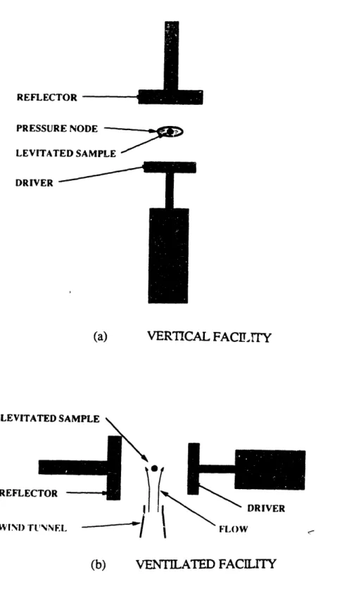
Depending on the particular experiment conducted, it may or may not be necessary to simulate the flow field around the hydrometeor in addition to simulating ambient temperature and humidity conditions. Consequently, two separate levitation facilities have been developed. In one, a vertically oriented acoustic levitator utilizes a strong acoustic field to support objects against the force of gravity. The configuration of this facility is depicted in Fig. 1-2 (a). The surrounding medium in which the suspended object is held is essentially motionless. In the second facility, shown schematically in Fig. 1-2 (b), a small vertical wind tunnel provides the levitating force on the suspended object. This force, arising from aerodynamic drag on the object, opposes the gravitational force on it. In this facility, a horizontally oriented acoustic field is used to stabilize the suspended object within the flow field of the wind tunnel. The

REFLECTOR PRESSURE NODE LEVITATED SAMPLE DRIVER (a) -. , VERTICAL FACILITY _; FL()W (b) VENTILATED FACILITY

Figure 1-2: _{Principle of operation of the two levitation facilities: (a) Vertical Facility, (b)} Ventilated Facility L1,VI I A REFLEC WINI) 'Ir DRIVER r cabrr . Adr o . . ,,

-motion of the surrounding medium is approximately that of the terminal velocity of the suspended sample.

Carefully controlled collisions between various particles are possible in the ventilated test facility. The primary advantage of utilizing acoustic radiation in this facility is that precise control of wind tunnel flow speed and turbulence levels is not required The acoustic field provides positional stabilization, and the suspended hydrometeor is therefore less sensitive to flow perturbations. In addition, the ventilated test facility is capable of accurately reproducing the flow field around free falling hydrometeors, with negligible secondary effects resulting from the acoustic field present.

1.4 Outline of the Thesis

The theory of acoustic levitation is presented in Chapter 2. The effects that give rise to the levitation phenomenon are described in detail. Based on mathematical models, predictions are made concerning the behavior of solid and liquid samples in the acoustic field. These effects include stability of samples held in the acoustic field and the deformation of liquid droplets. In Chapter 3, the major design issues concerning the development of the acoustic levitation hardware are discussed. Certain criteria are cited that ensure proper operation of the apparatus. A detailed description of the baseline acoustic levitator is then presented, along with the relevant operating parameters of the device. Chapter 4 describes in detail the vertical and ventilated facilities. Critical design issues concerning the implementation of acoustic levitation in each facility are studied. The calibration and operation of both facilities is discussed. A series of validation experiments are conducted in Chapter 5. The limitations of the facility are compared with the theoretical predictions. These experiments include studies of the levitation limits on solid and liquid hydrometeors, the effect of the acoustic field on molecular diffusion processes, and the effect of shape distortions of water droplets arising from the acoustic field on terminal velocity in free fall. Conclusions and recommendations are presented in Chapter 6.

Chapter 2

Theory of Acoustic Levitation

2.1 Introduction

Qualitatively, the net force on an object subjected to an acoustic field arises from the nonlinear relationship between the instantaneous pressure and velocity in an acoustic medium. Under certain conditions, this nonlinearity can produce significant pressure gradients over the surface of an object, resulting in an appreciable net force on it. As a result, sufficiently strong acoustic fields can suspend objects against the force of gravity, making it possible to study the objects in a contact-free environment

In this chapter, numerical and approximate analytical expressions are derived for the net force on a rigid sphere in an acoustic standing wave. Stable locations within the acoustic field are then determined for both gravity-free and l-g environments. The effect of the acoustic field on liquid samples is also important, as many cloud physics experiments involve liquid water. As a result, a mathematical model is developed and used to predict effects such as droplet deformation, oscillation, and shatter.

2.2 Levitation of Solid Objects

In order to study the effects of a planar acoustic field on an object of arbitrary shape, it is useful to first analyze the simple case of a rigid sphere placed in such a field. By making several reasonable approximations (discussed in the sequel), .a analytical solution to this problem is available. The net acoustic force on a rigid sphere is then readily calculated. This result can then be extended to oblate or prolate spheroids without significant loss in numerical accuracy, provided that these spheroids do not deviate significantly from spherical. These small deformations are characteristic of naturally occurring hydrometeors, such as raindrops and graupel particles. For these cases, the net acoustic force can be approximated as the force on ar. equivalent sphere (defined such that the volume of the sphere equals the volume of the

spheroid). For more complex geometries, the results from the simple spherical analysis can be used to predict only general trends, such as the maximum allowable object dimensions for which acoustic levitation is possible.

In light of these arguments, only the simple case of a rigid sphere in a planar acoustic field is studied here. More complex models, which consider more arbitrary geometries do not enhance the understanding of the physics of acoustic levitation significantly, and are not developed here.

2.2.1 Net Acoustic Force on Rigid Spheres in a Planar Standing Wave

In order to develop expressions for the effect of an acoustic field on a spherical object placed within it, it is necessary to solve the wave equation in three dimensions with appropriate

boundary conditions. The development presented here is based on theoretical work done by. Louis King in 1934 [1]. In his paper, King developed approximate acoustic force expressions for both travelling and standing waves. King showed that the forces arising from travelling waves are significantly smaller than those arising from planar standing waves. As a result, only standing waves are considered here. The theory developed by King specializes to the case where the radius of the spherical object is significantly smaller than the acoustic wavelength. This makes it possible to derive an appreoximate analytical expression for the acoustic force. The theory presented here applies to spheres of arbitrary size, and involves a numerical computation of the net acoustic force rather than an approximate analytical expression.

In the subsequent development, an approximate expression for the local pressure variation (p) in terms of the velocity potential (D) is derived. The velocity potential is then expressed as the superposition of the incidental planar standing wave and the divergent scattered wave. Upon application of the boundary conditions at the surface of the spherical obstacle, the wave equation is solved exactly. The pressure variation along the surface of the object, averaged over one period of the standing wave, is then determined. Upon integrating this variation over the surface of the sphere, the net force due to the acoustic field is found. An

approximate analytical expression for this force is developed for small spheres to check for consistency with the King theory, and a numerical method is used to determine the force on larger objects.

2.2.1.1 Problem Description and Boundary Conditions

Given the geometry of the problem to be solved, as shown in Fig. 2-1, it is clear that a spherical coordinate system (r,0,0) is appropriate. The origin of this system lies at the center of the spherical object, with the line 0=0 normal to the planar standing wave. This line

corresponds with the z-axis of the related Cartesian system. We will assume that the object lies a distance h above a velocity nodal plane. Alternatively, we may say that a velocity nodal plane exists at z = -h.

We now define the velocity of the acoustic medium at any point by

A AA

v=v r r + Vov+ vo (2.1)

Clearly, from the symmetry of the problem, v, = 0 everywhere. For our purposes, the acoustic medium can be modeled as a compressible, irrotational fluid. This guarantees the existence of a velocity potential, d, which relates to the velocity of the fluid as follows:

aI~ 1 a

Vr=

='ao

I(2.2)

vr=9j

Ve-r

v

If we denote q2 = v2 + v + v, we see that

q2=^)

2

_+r2(~)

_(2.3)

Because the fluid must remain in contact with the spherical obstacle, we have the boundary condition

vr

r=-

I=

=

a2

i

r

=

a12

(2.4)

z

0

z

1

t/

1/2

Nodal Plane

Nodal Plane

Figure 2-1: Geometry of the acoustic levitation problem: (a) spherical coordinate system, (b) position of the sphere with respect to the nodal plane of standing wave.

' co::fi: [Si ..r..X ,I I I IN _ _ _ J [ `11

where a is the radius of the sphere. Making the substitution g = cos 0, we obtain

q

*

a

2

_{rIXa a}

_[

_r,

_(2a

_a

_{si2lr =}

_a

_(2.5)

which leads to

2 (1

J

q21= a- a

We must now express the pressure deviation, Sp, in terms of q and D. We make the assumption that the acoustic medium is barotropic (i.e., p is a function of p only). For this case,

p1 2 1 P 2 (2.7)

SPp a PO - 2 Po 2

The details of the derivation of this expression are presented elsewhere [1]. It should be noted that Eq. (2.7) is correct to terms of the order q /c2. Even at large acoustic energies (140dB, for example) the ratio q/c remains small, so that the expression for the pressure variation, given by Eq. (2.7), is a reasonable approximation1.

Throughout this development, it is assumed that the center of the sphere is fixed in inertial space. This results in the simple expression for the boundary condition given by Eq. (2.4), since it is assumed that the radial velocity of the fluid at the sphere's surface is the same in an inertial frame as it is relative to the motion of the sphere. The first term in Eq. (2.7) does not contribute to the net acoustic force when time-averaged over one period of the standing wave. However, at any particular instant, this term dominates over the other two. Because the acoustic field varies sinusoidally in time, the force arising from the first term in Eq. (2.7) exhibits the same temporal variation. As a result, within one period of the acoustic field, the

lThis can be verified by expressing q/c in terms of the relative pressure ratio, 6p/po. It can be shown [4] that the approximate relationship is q/c - (l/y)(Sp/p), where y= 1.4 is the gas constant for air. At an intensity

level of 140 dB, the approximate value of 8p is 200 Nt/m2, while po at sea level is approximately 105 Nt/m2.

object translates in a direction perpendicular to the nodal plane (i.e., along the z-axis) in a sinusoidal manner. Consequently, over time scales shorter than the period of the acoustic field, the center of the spherical object is not quite inertial. Nevertheless, it can be shown that, for a sufficiently dense object, this translational motion is insignificant. Denoting r as the displacement of the spherical object along the z-axis and taking into account only the first term in Eq. (2.7), the equation of motion of the object over short time scales can be approximated as follows:

4 3 2

ra3plt = -f

Jp

P

00

0. 0

where Pi represents the density of the spherical object. This equation can be solved for , yielding,

1

C(t

Of d

(2.9)

The sinusoidal time dependance of th.'s motion becomes apparent by noting that the velocity potential itself varies sinusoidally, with frequency corresponding to that of the acoustic standing wave. The important factor in Eq. (2.9) is the ratio po/pl, which relates the

magnitude of the acoustic force to the mass inertia of the object. For objects of interest (water droplets, ice crystals, etc.), this ratio is small, indicating that the motion of the object subject to the sinusoidally varying pressure force is negligible over times scales longer than the period of the acoustic field. An analysis which takes into account this motion has been performed by King [1], with the conclusion that, for small po/Pl, the motion is indeed negligible.

The second and third terms in Eq. (2.7) contribute less acoustic force over short time intervals. However, because the first term integrates to zero on the average, it is the effects of these two terms that give rise to a steady-state acoustic force on the object, and, hence, the

capability for acoustic levitation. Taking the ime average of the pressure variation over one period of the standing wave, we have, on making use of Eq. (2.6) and Eq. (2.7),

Sp Ir= pODI = a - (1· )y -2cr[j

a]+

1

2.2.1.2 General Solution of Wave Equation

The wave equation to be solved for this problem is given by:

2 _V2 (2.11)

c at

which is the familiar wave equation in three dimensions. This equation is based on several underlying assumptions. The first is that the flow is irrotational. The second is that the speed of sound, c, in the medium is a constant, given by c2 = dp/dp. For sufficiently small fluid velocity (q << c), it can be shown that both approximations are reasonable [5].

The general solution of this wave equation for this problem must now be determined. For the particular case of a spherical object within a planar standing wave, it is obtained by superposing the respective potentials of the incident and scattered waves. This yields a solution of the form:

=

I

A

(kr)

+

A (kr)

_{A(kr) }}

_(2.12)

where k = o/c, o = 2if and Sn is a surface harmonic of order n. The coefficients An and A;

depend on the boundary conditions of the particular problem to be solved. The obvious restriction that the surface harmonics be finite in all directions restricts the set of possible

surface harmonics to the Legendre polynomials Pn() The terms iVn(kr) and fn(kr) are spherical wave functions appropriate to the expressions for the incident and diverging waves, respectively. It can be shown [5] that, for a diverging wave, the wave function can be expressed as:

fn(x) = n(X) - jVn(X) (2.13)

where $n(x) is also a spherical wave function. The series expansions of these functions can be found from their corresponding recursion formulas. They are as follows:

1 + _(2.14)

Vn(X) 1.3 .... (2n+1)n 2(2n+3) 2.4.(2n+3)(2n+5.14)

(x) -

xn+l

Considerable use is made of the following relations satisfied by In(x) and On(x)

- -xVn+l (x), - -Xn+l(X)

*n(x) Vnjl(X) - Vn(X) n+l() 1/X2n+1

,n+l()

n-(X )

The velocity potential then becomes:

0

n n

n (kr) + Am

q(kr)

P( )

(2.17)

In order to facilitate the determination of the remaining coefficients, it is useful to make the substitution:

n 1 _(2.18)

A- F/G

-j

The ratios Fr/G_n then become the unknown constants. Both F_n and G_n depend only on the nondimensional parameter, a , defined by a = ka, where a is the radius of the spherical object and k is the acoustic wave number. The appropriate form of the velocity potential then

becomes:

'=EA)

'

Gnnnr

Fn- jGn

n = 0

2.2.1.3 Application of the Boundary Conditions

The boundary condition at the surface of the sphere is that the component of the velocity in the radial direction is zero. This follows from the fact that the fluid must remain in contact with the surface of the sphere. Making use of Eq. (2.4), we find:

00

cn n n

a Ira

=

A

[

Fn

G (a)}

r(a)n

1

n=O

+ Fn+F- n k"

rn

p

0

Fn - n

which reduces to:

(nWn- a2V]n+l) F = (non- a 2On+l) Gn (2.21)

This relation leads to the following choices for Fn and Gn:

These choices are not unique, as only the ratio Fn/Gn is used in the expression for the velocity

potential. At the surface of the object, we have kr = ka = cL Making use of the wave function properties (2.16), we get:

A P ()

n+l F - iG (2.23)

n=O

At this point, only the coefficients Anneed be identified. These relate to the incident

acoustic field. The velocity potential for the incident standing wave can be represented in Cartesian coordinates as:

(Q. = Ae cos k(z+h)) (2.24)

or,

i= 1 Aet (ekhejkz

+ ekhejkz)

(2.25)

It will be necessary to express this potential in spherical coordinates. To do this, we make use of the identity:

00

eJkz=

:

(2n+l)

(jkr)n P(pg)

(2.26)

The incident potential then takes the desired form:

o00

(D = A n (kr) (kr) Pn(R) (2.27)

where:

A = Aeot (2n+1) cos (kh + I nr) (2.28)

The total potential at the surface of the spherical object then becomes:

2n+@1

0PO0

4)

I_

n

_--

_X2n+2

_F-jG

Making the substitutions:

1 F F(a) cos

n+ln

Sn ( a (n+I F2() + 2 cos (kh +

2

n n

results in an even simpler form:

@0

r

r

=A cos(ot) +j sin(rx)

_Rn

_{-j Sn(a)} P()}

_(2.31)

n=O

Henceforward, the dependence of Rn and Sn on a and the dependence of Pn on g will be

assumed. Taking the real part of this expression, we get:

4 )

=A

cos (ot)

R nP + sin (ot) P S

n

P

(2.32)

n=

n= 0

2.2.1.4 Determination of Pressure Variation Over Surface of Sphere

We must now manipulate Eq. (2.32) into several forms, which can be substituted into Eq. (2.10) to obtain a formula for the pressure variation over the surface of the spherical object. From (2.32), we obtain

Ir = Ao -

sin (ot)

R P + cos (cot)

E

S P

00 -2

nR

= A202sin2(t)

+ cos

(ot)

SnPn

n= 0

-2 sin (ot) cos (ot)

2

= A2 os2(ct)

IRnP

n n

[ 0RnPn

I SnPnJ

+ in t) SnP

+ 2 cos (tot) sin (tot)

These expressions, time-averaged over one period of the standing wave, become:

Ir= a.

=0

[ Ir =a]

:-2

{ [I

RnPn] + [

SnPn]

2A2{ RnPn2+

[

Upon substitution of Eq. (2.34) into Eq. (2.10), we have, for the time-averaged surface pressure variation, 2 BP = -2 _4a2 U(a,l) (2.35) where

(1-]g

_{) {}

_[n

_o

_{+ [}

_{SnPn] }(2.36)}

ao

I-a-r

This expression is used in the sequel to predict the deformation of a liquid sample in the acoustic field due to a pressure gradient over its surface. It is also possible to numerically integrate this expression over the surface of the object to obtain the net force on it. However, an analytical approach, which exploits some orthogonality properties of the Legendre

Polynomials, produces a more useful result.

2.2.1.5 Net Effect of Acoustic Pressure Distribution on Sphere

We seek an expression for the net force on the object along the z-axis, time-averaged over one period of the standing wave, defined as P. This is obtained by integrating the component of the time-averaged pressure variation (p) in the direction of the z-axis over the entire surface of the sphere. Hence:

2R Jt

P =

-

I (p

cos

0)

a

_{sin d d}

_(2.37)

00

where the overbar ( ) denotes integration with respect to time over one period of the standing wave. From Eq. (2.35), we obtain,

1

P =-2p Xp

f U(a,{l)

d

(2.39)

-1

-1 0 n > n+l

l1n 2n(n+ )(n+2)

J(1-R

_{P'm(L)dg = (2n+1)(2n+3) m}

_(2.41)

-1 0 m > n

As a result, the expression for the net acoustic force takes the form,

00

P = 27rpA2 _{n+1 R{} 2

_nn

(2n+1)(2n+3) RnRn+l+ _{SnSn+ } { a -n(n+2) (2.42)}

n-=0

Making use of the definitions of Rn(a) and Sn(a), we obtain, after some manipulation,

R R _R +S

S

n n+ SnSn+ 1 2a 2n+3 [FInG2] [ (2.43)

Finally, combining Equations (2.42) and (2.43), fwe obtain,

2

P = - p A sin (2kh) T(a) (2.44)

where,

T(a)._

(_l)n n+l '/

_{T(a)= (-1)}

_{] [Fn2}

_{] a}

2

_n(n+2)}

_(2.45)

2-45G)

n=O

The function T(a) can be regarded as a normalized acoustic force. This function represents the dependance of the acoustic force on the size of the suspended sphere for a given acoustic field strength. It is interesting to note that the net force varies sinusoidally with h, the distance between the center of the object and the nodal plane of the standing wave. We see that there are two points within each wavelength for which the force is maximized, corresponding to kh =

number of terms to obtain an explicit value for the force on a spherical object placed within the acoustic field.

At this point, it is appropriate to compare the results obtained by King [1] with the theory developed here. For small objects (ac<<1), an approximate expression for the net acoustic force is readily obtained. We have, for small a,

1 2 9

a

FO~ {i, 1 a3'F2-5 tc.-, GnGn+l << FnFn+l (2.46) which leads to

T(a) a << 1 (. 2.47)

and

P . 56 Irpo A2 acsin (2kh), a << 1 (2.48)

This result is consistent with results from King's work on acoustic levitation. It is interesting to note that the acoustic force on small spherical objects varies as the cube of the object's radius. Since the mass also varies as the cube of the radius, objects of all sizes (all having the

same density) will be accelerated uniformly in the presence of the acoustic field. Furthermore, this indicates that the ability to suspend small objects against gravity depends only on the energy of the acoustic field in relation to the density of the object, irrespective of the size of the object. Note that this effect is valid only for a sphere with diameter considerably shorter than the acoustic wavelength, corresponding to the case where a << 1.

It is useful to express Eq. (2.44) in terms of the time averaged energy density of the acoustic field, defined as E. By making the substitution E = 2 pok2_A2_{, which relates the}

energy density of a standing wave to its amplitude, we obtain

E

2.2.1.6 Levitation Limit for Large Spheres

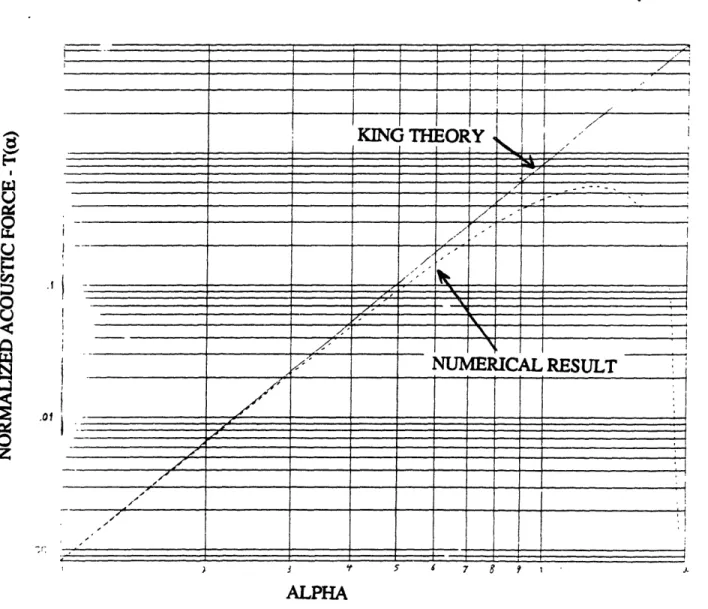
For larger objects, the net acoustic force is approximated using Eq. (2.45). In Fig. 2-2, the nondimensional acoustic force, T(a), is plotted against a so that the approximation for small objects can be compared with the more accurate numerical result. It is apparent that the approximation is valid for oa < 0.5. Beyond this point, the net acoustic force falls off rapidly with increasing sample size. It is clear that, as a approaches 2, the net acoustic force vanishes. This point represents the fundamental theoretical limit to acoustic levitation, as the acoustic energy required for suspension against gravity approaches infinity. This rapid reduction in levitating force is related to the fraction of the acoustic wavelength spanned by the spherical object. As the parameter a becomes larger, the upper and lower surfaces of the object enter regions of the acoustic field where the local pressure deviation diminishes the net acoustic force. For sufficiently large a, this effect eventually cancels the net upward force arising from the pressure deviation near the equator of the object

In order to support this claim, the pressure distributions over the surfaces of spheres of several sizes were computed numerically. The model assumes each sphere to be located at the point of maximum net acoustic force (kz eq--4). For each trial, the acoustic energy was selected to provide a net force equal to the weight of the sphere. The results are displayed in Fig. 2-3. In this figure, the normalized pressure deviation from ambient is plotted in inverse polar coordinates as a function of the location along the surface of the sphere. The plots help to visualize the pressure distribution, and provide insight into the relative magnitude of the

distribution over the sphere. In the absence of any pressure deviation, the plot reduces to a unit circle. In regions of increased pressure, the radial coordinate is less than unity, indicating that the net acoustic force in these regions is directed inward (i.e., toward the center of the sphere). Conversely, in regions of diminished pressure, the radial coordinate is greater than unity, indicating that the net force is directed outward (i.e., radially from the sphere). Using this convention provides a direct visual correspondance between the distribution of the pressure

8

.

.01

ALPHA

Figure 2-2: Normalized acoustic force on a sphere as a function of cL The solid line represents the approximation for small a, while the dashed line represents the more precise numerical solution. Note the rapid falloff in acoustic levitating capability for a > 1.

" t ~ "' -" ' I - \

(f)

(a) a= 0. 1

-I

(c) o = 0.5

Figure 2-3: Visualization of the distribution of pressure forces over surface of spheres of different sizes. Plots (a) through (h) correspond to a = 0.1, 0.2, 0.5, 1.0, 1.2, 1.4, 1.5, 1.6, respectively. In all cases, E = 1. For each polar plot, the radial coordinate corresponds to the nonnalized magnitude of the local pressure force. Points

on the unit circle correspond to a local surface pressure pressure equal to the ambient value. Over regions of increased pressure, the radial coordinate is less than unity, indicating a net inward force on the sphere. Over regions of decreased pressure, the radial coordinate is greater than unity, indicating a net outward force. The relationship between the pressure and the radial coordinate is linear.

I II

i ,I LI -

2:

1--< '- I "-I,,-,-I .. 1--x,

-I

_It·

forces and the resulting effect on deformable samples placed in the acoustic field, such as water droplets (See Section 2.3). For small spheres (a<l), the pressure distribution is rather well-behaved, with the net upward force arising from both increased pressure below and reduced pressure above the sphere. However, for larger values of a, a region of increased pressure develops above the sphere, which eventually cancels the upward force from below. This explains the sharp decrease in levitating capability for larger objects.

2.2.2 Stability of Spheres in Acoustic Levitation Environment

We must now determine the equilibrium position of a sample suspended in the acoustic field. To do this, it is useful to fix the coordinate system to the nodal plane below the sample. The coordinate z is then redefined as the time-varying distance of the center of the sample from the nodal plane of the standing wave. The equation of motion for the sample can then be expressed in terms of z. It should be noted that, for the case of a pure standing wave, neutral stability exists in all directions parallel to the nodal planes.

2.2.2.1 Gravity-Free Environment

In the absence of gravity, the only force acting on the suspended object is that of the acoustic field. Force equilibrium requires that:

e t 2k n(2.50)

Zeq 2k

where n is an integer. The stability of each equilibrium location can be assessed by analyzing small perturbations from this equilibrium condition. Denoting the deviation of the sample from its equilibrium location by Sz, we obtain

E

BP = 2 T (x) sin [2k(zeq+8Z] (2.51)

P = 4n (-1)nT (a) z =- 4ra3 pl

S

The resulting equation of motion then becomes

8z + (-1)n+l 3T(o) Ek2 _(2.53)

a3 P1

It is apparent that the motion is stable only when n is odd. Thus stable nodes exist at Zeq= 7c/2k, 3/2k, etc. These correspond to the pressure nodes (or velocity antinodes) of the acoustic standing wave.

In the presence of disturbances, the sample will oscillate about its equilibrium position in a direction normal to nodal plane. The frequency of this oscillation is given by:

o

= (2.54)

a P1

For small samples, we may use the expression given for T(a) in Eq. (2.45). Thus,

(2.55)

2.2.2.2 Levitation Against Gravity

With gravity directed normal to the standing wave, the equilibrium location is below that which exists without gravity. Equating forces, we have:

4 3 =nTE

3ia plg = 2 sin (2kzeq )T(a) (2.56)

s

[-(

)

(

Ek)]

(lower

equilibrium)

2kz

t

l

3

-o

si(a)n

Ek

(upper equilibrium)

As shown in Fig. 2-4, the lower equilibrium location is unstable. If the object is perturbed from this location in the downward direction, it moves into a region of reduced levitating force. As a result, the net force on the object is downward, causing it to be accelerated in that

direction. The acoustic force is therefore further diminished. The reverse is true for perturbations in the upward direction. Hence, the lower equilibrium position is unstable. Conversely, the upper location given by Eq. (2.57) is stable. Here, small perturbations result in acoustic restoring forces which return the object towards equilibrium. From Eq. (2.56), it follows that the minimum acoustic energy required for levitation against gravity is given by

Emin 3 kr(o) (2.58)

For small objects, it is again possible to approximate T(a) by Eq. (2.52). This yields, for small samples,

Emin 5(4 ) I (2.59)

As expected, the minimum required acoustic energy depends only on the wavelength of the acoustic field and the densities of the sample and surrounding medium.

A useful nondimensional parameter associated with levitation against gravity is the ratio of the acoustic energy density present to the minimum value required for levitation. Thus, defining this factor as E = E / E min' the equilibrium condition becomes

LJ u ~~~~~~~~~~~-I

D U

I:

en

II

-

I I

I<

1

_I

1<

14

3

z

0

I

IF_0.

Iz

I

<I

_{| < 1}

₈

I

₁₁₈

z

-J

0.

z

-The use of this parameter simplifies the equation of motion of the sample for small oscillations about equilibrium. For small perturbations from equilibrium, we have, from Eq. (2.56) and Eq. (2.60),

4 a3p, P z - 3 4+ 3_{pg sin 2k(zeq+z)] E}

[7ia

which, after linearization, yields

4 3 ' 8 3

4 Ia p

I

The resulting equation of motion is then

6 + 2gk '

Iz-0=

(2.63)

From this equation, we can infer that, in the presence of gravity directed normal to the nodal planes of the acoustic standing wave, the frequency of oscillation of a levitated sample about its equilibrium position in that direction is given by:

D0)

=40

2

fk

(2.64)

2.3 Levitation of Liquid Droplets

It is important to study the effect of the acoustic field on liquid droplets as well as solid objects. It will be shown that, for sufficiently large droplet diameters, surface tensions forces will be inadequate to maintain droplet stability. As a result, large droplets will shatter in the acoustic field. For liquids, this limitation is more constraining than the rapid falloff of levitating force with increasing sample size described in Sec. 2.2.1.7. The deformation limitation is quantified here. This problem is compounded by the possible dynamic effect of induced droplet oscillations in the acoustic field. The excitation of one of the fundamental modes of the droplet due to acoustic effects will, most likely, cause the droplet to shatter prematurely. As a result, this issue is addressed here as well.

2.3.1 Distortion of Droplet Shape from Spherical

When a liquid sample is suspended within the acoustic field, its shape will deform due to the nonuniform pressure distribution at its surface. For large droplets, the surface tension of the fluid may not be large enough to prevent the sample from shattering. The following

development attempts to quantify this limit. The theory presented here has been used in earlier work [6] which examined the equilibrium shape of water droplets in free fall, and assumes that the pressure distribution over the surface of the droplet is known. It is also assumed that the droplet is suspended against gravity.

2.3.1.1 Mathematical Model

Initially, it is assumed that the droplet is spherical, so that the acoustic pressure over its surface can be readily obtained from the theory presented in Sec. 2.2.1. By equating internal and external pressures with surface tension forces, an equilibrium shape is determined. The deviation of this shape from spherical results in new boundary conditions for the wave

equation of the acoustic field, which will result in a new distribution of acoustic pressure over the surface of the droplet. However, it will be assumed that, for small deformations, the change in the pressure distribution is negligible. Without this simplification, it would be necessary to solve the acoustic wave equation for a general droplet shape, which is neither instructive nor practical. The initial deformation of the droplet from spherical will be adequate in determining droplet stability within the acoustic field.

In the following development, only acoustic, hydrostatic and surface tension forces are taken into account. Circulation internal to the droplet, as well as ambient flow disturbances, if present, are not modeled. The geometry of the deformed droplet is shown in Fig. 2-5.

By balancing forces at the surface of the droplet, we can write

[R 1(0) R(O)] Pi( ) p() (2.65)

Figure 2-5: Deformation geometry of a liquid droplet. It is assumed that the droplet is radially symmetric about the vertical axis (0 = 0).

where R1 and R2 are the local principal radii of curvature of the droplet. Replacing Pi with the

local hydrostatic pressure, we obtain

[R (O) + R2o

]

where Pi(O) represents the internal pressure at the upper surface of the droplet, po represents the ambient atmospheric pressure in the absence of an acoustic field, and Sp = p - po. In order to convert this equation into a form that can be numerically evaluated, it is necessary to express both r(O) and

Sp(O)

r=a@ + C cos n

r =a (1 +

c

(2.67)

n = O n = O

8p(0) - 2 _{U(t, cos ) = 2}

_cos

_nO

(2.68)

4a2 4a n

Making these substitutions, Eq. (2.66) becomes

a[R

n

- cos

os

cn os

0

cos nO)

2

-Ž.... qn cos nO (2.69)

n =O

A relation between the radii of curvature and the coefficients cn of the deformation is needed. In earlier works [7][8][9], Imai, Savic, and Landau showed that, for reasonably small

) + R2(O) J() R 1() 'r R 2 .

J()= 2 +

(n2-2)cncosnO+

ncn

At this point, two nondimensional parameters, the bond number (NBO) and an acoustic number (NAC) are introduced They are defined by

2

ga pA 2k

NBO = ' NAC 4ca The equation for force balance then becomes

(2.72)

J() = NBO 1+ Cn - Cos - nCOS Cos nO )- NAC

n=O n=O

I

qncos n(2.73)

n =

which can be manipulated into the following form:

K-BO YCn

+

NBO c[Cos (n+l)0 + cos (n-l)O] +

n=O n=O n

Z

+

Znc

K=2-NBO +NBO cos

By exploiting the orthogonality of the cosine series, it is possible equate terms in cos kO. This yields the following relationship among the coefficients:

where

(2.70)

(2.71)

where

2 NB (k l+ ck.1) + (k2-2) k +

k

2

k-

The coefficient cl corresponds to rigid body motion in the vertical direction, and is therefore set to zero for our purposes. These equations can be written in matrix form if the series expansions are truncated after several terms. In this numerical model, only terms up to cos 90 are considered. The resulting matrix equation is therefore

q2 4N8

012

016

N

C5

N27

6

c7

7

where N -= NBO. The constant term, co, can be found by invoking conservation of volume, treating the droplet as incompressible fluid. We have, for the volume of the deformed droplet,

V

=f

J J

sin 0 dr dO d

=

(2.78)

00 0

0

Substituting the series expansion for the droplet radius, we e9tain the approximate expression

V _I3 a +2 aJI

cn cos nO sine dO

(2.79)

which holds for reasonably small deformations. For an incompressible sample, this volume must equal the original volume of the sphere. This leads to the constraint:

T fc cos nO sin 0

dO

n=O

Isolating the first term yields

00 c

c= -2

c

n=2

Using the trigonometric formula

-2 n even

cos nO sin 0 do = n2 1 (2.82)

L 0 nodd

produces the desired result:

co0 4n2 1 (2.83)

1

At this point, it is possible to predict the equilibrium shape of any liquid object suspended in the acoustic field. The solution is a function of four non-dimensional parameters. These are: P /Po, a, E, and NBO. The acoustic number, NAC, can be expressed in terms of NBO and a as

_N =I B (2.84)

NAc - 3 T(a)

These four parameters are all that is required to completely specify the problem. Assuming that the ambient fluid is air and the droplet is liquid water, the ratio pl/p0o is fixed. Also, at a given

acoustic wavelength, the droplet diameter determines both a and NBO' The only other parameter that can be varied is E, which is directly related to the acoustic field strength. The

shape of a levitated droplet of water in a given acoustic field is therefore characterized by the two parameters, a and E.

2.3.1.2 Predictions Based on Mathematical Model

A numerical model was developed that determines the theoretical shape deformation of a droplet under acoustic levitation. The model computes the equilibrium location of the droplet within the acoustic field, and determines the pressure distribution at that location. Based on this distribution, an equilibrium shape is found. In order to study deformation effects arising from various acoustic field strengths, the theoretical droplet size was held constant at a value corresponding to a = 0.7, and the acoustic energy was varied from E = to E = 1.7. The resulting pressure distribution and equilibrium shape for each trial is shown in Fig. 2-6. At the minimum energy required for levitation, a diameter water droplet whose diameter corresponds to a = 0.7 is only slightly distorted. Its top surface is flattened, and its sides are stretched outwards. However, at energies only slightly larger than this minimum value, more severe distortions appear. The upper and lower surfaces become concave, and the droplet as a whole becomes much more flattened. At this point, the local curvature of the droplet at its upper and lower surfaces is quite acute. It is assumed that the surface tension of the actual droplet will be inadequate to maintain stability. At this point, it is predicted that the droplet will shatter under the combined effect of acoustic and gravitational forces. This phenomenon is not part of the model.

It is apparent that, for a given droplet size, there exists a maximum acoustic field energy for which the droplet will not shatter. In order to quantify this relationship, it would be useful to define a parameter characteristic of the magnitude of the deformation. An appropriate choice is the droplet aspect ratio. It is defined as the ratio of the maximum thickness of the droplet in the direction normal to the standing wave to its maximum diameter in the direction parallel to the nodal plane (See Fig. 2-7). The predicted aspect ratios for droplets of various sizes under varying acoustic energies were determined from the model presented above. The results are

(a) E = 1 '.5 1- T -(b) I,; / , ~ 1 / , I ~I \, 2 /'

E= 1.2

Figure 2-6: Deformation of a water droplet from spherical under the combined effect of gravity and acoustic forces. The inverse radial pressure distributions are shown atleft and the couesponding deformed shapes are shown at right for: (a) E = 1, (b) E = 1.2, E =

1.45, E = 1.7. The value of a is 0.7 for all cases. Note the large shape distortions predicted for higher acoustic energies.

2b

-A-L

-

Figure 2-7: Definition of deformed droplet dimensions. The aspect rtio is defined as b/a, and the equivalent radius is (for small deformations) approximately a

I I

presented in Fig. 2-8. As expected, the droplet shape deteriorates rapidly as the acoustic field strength is increased above the minimum value required for levitation. This implies that, in order to maintain droplet stability, the value of E should be only slightly larger than unity. However, at this level, the droplet is only marginally stable, and transients in the acoustic field will cause the droplet to fall. It is therefore necessary to have excess power in the acoustic field. Thus, a reasonable lower limit for the acoustic energy is E = 1.2. The theoretical droplet aspect ratio which corresponds to the anticipated shattering of the actual droplet must be

estimated. Referring to Fig. 2-6, it can be inferred that droplet shatter will occur at a theoretical aspect ratio of about 0.5. Finally, from Fig. 2-8, it can be concluded that the largest droplet that can be supported has a value of a equal to 0.85. As expected, this value represents more of a constraint on the size of the droplet capable of being levitated than does the sudden falloff of levitating force for large solid objects.

It is important to note that this theoretical limit is valid only for levitation against

gravity. In the absence of gravity, a considerably weaker acoustic field is sufficient to stabilize the liquid droplet. The field strength need only be large enough to prevent loss of positional stability of the droplet in the presence of flow turbulences in the ambient medium. As a result, larger droplets can be suspended within a gravity-flree environment without risk of droplet shatter.

2.3.2 Droplet Oscillations in the Acoustic Field

As described in Sec. 2.2.2, the restoring force of the acoustic field on a suspended droplet causes the droplet to undergo oscillations about the equilibrium position in a direction perpendicular to the nodal plane. This creates the potential for excitation of one of the

fundamental oscillatory modes of the droplet itself. These oscillations arise from interactions between viscous and inertial forces within the droplet and sur, tension forces over its boundary. It has been shown in many texts [10] that the first oscillatory mode of a droplet is given by

ui

0

Figure 2-8: Predicted aspect ratio of droplets of various nondimensional size subjected to various acoustic energies.

1 = iPla3 (2.85)

where a is the radius of the droplet, and a and p are the respective surface tension and density of the droplet.

In the absence of gravity, the acoustic force required to keep the droplet stabilized is low compared to the corresponding case for levitation in the presence of gravity. The acoustic field strefigth need only be sufficiently strong to prevent ambient disturbances from forcing the

sample out of the acoustic region. Because the frequency of droplet motion about the nodal plane induced by the acoustic field decreases with decreasing field strength, it is expected that the frequency of this oscillation will be well below the first resonance of the droplet for the required acoustic energies anticipated in a gravity-free environment.

For levitation against gravity, on the other hand, the oscillations induced by the acoustic field must be considered. Here, the energy of the acoustic field will be much higher, so that the sample can be suspended against the force of gravity. As a result, the fiequency of the oscillations induced by the acoustic field will be significantly higher than would be the case in a gravity-free environment. Using Equations (2.63) and (2.82), the relationship between the fundamental oscillatory frequency of the droplet and the frequency of oscillation induced by the acoustic field can be compared The results are graphed in Fig. 2-9. From the graph, we conclude that excitation of the fundamental mode occurs only at extremely large values of , and then only for large droplets. In these regimes, it is anticipated that the pressure forces alone will be sufficient to cause shattering of the droplet without the added effect of droplet motion. Consequently, it is expected that induced droplet oscillation will not occur for droplets of diameters in the range of interest.

It should be noted that, if desired, others methods are available for intentionally inducing droplet modal oscillations. The most direct method, for example, would be to modulate the intensity of the acoustic field at the desired frequency. The magnitude of the pressure forces on the droplet would then vary sinusoidally over the droplet surface, and shape