HAL Id: hal-01870512
https://hal.inria.fr/hal-01870512
Submitted on 7 Sep 2018
HAL is a multi-disciplinary open access
archive for the deposit and dissemination of
sci-entific research documents, whether they are
pub-lished or not. The documents may come from
teaching and research institutions in France or
abroad, or from public or private research centers.
L’archive ouverte pluridisciplinaire HAL, est
destinée au dépôt et à la diffusion de documents
scientifiques de niveau recherche, publiés ou non,
émanant des établissements d’enseignement et de
recherche français ou étrangers, des laboratoires
publics ou privés.
Digital surface model generation from multiple optical
high-resolution satellite images
Lionel Mattéo, Yuliya Tarabalka, Isabelle Manighetti
To cite this version:
Lionel Mattéo, Yuliya Tarabalka, Isabelle Manighetti. Digital surface model generation from
multi-ple optical high-resolution satellite images. SPIE Remote Sensing, Sep 2018, Berlin, France.
�hal-01870512�
Digital surface model generation from multiple optical high-resolution
satellite images
Lionel Mattéo*
abc, Yuliya Tarabalka
ac, Isabelle Manighetti
aba
Université Côte d’Azur,
bGeoazur UMR 7329, Observatoire de la Côte d’Azur, Valbonne France;
c
Inria Sophia Antipolis-Méditerranée, TITANE Team, France.
ABSTRACT
The modern optical satellite sensors capture images in stereo and tri-stereo acquisition modes. This allows reconstruction of high-resolution (30-70 cm) topography from the satellite data. However, numerous areas on the Earth exhibit complex topography with a lot of “discontinuities”. One case is tectonic fault sites, which form steep topographic escarpments enclosing narrow, deep corridors that mask parts of the ground. Built with common approaches (stereo or tri-stereo), a digital surface model (DSM) would not recover the topography in these masked zones.
In this work, we have settled on a new methodology, based on the combination of multiple satellite Pleiades images taken with different geometries of acquisition (pitch and roll angles), with the purpose to generate fully-resolved DSMs at very high-resolution (50 cm). We have explored which configurations of satellites (i.e., number of images and ranges of pitch and roll angles) allow to best measure the topography inside deep and narrow canyons.
We have collected seventeen Pleiades Images with different configurations over the Valley of Fire fault zone, USA, where the fault topography is complex. We have also measured sixteen ground control points (GCPs) in the zone. From all possible combinations of 2 to 17 Pleiades images, we have selected 150 combinations and have generated the corresponding DSMs. The calculations are done by solving an energy minimization problem that searches for a disparity map minimizing the energy, which depends on the likelihood for pixels to belong to a unique point in 3D as well as regularization terms. We have statistically studied which combinations of images deliver DSMs with the best surface coverage, as well as the lowest uncertainties on geolocalisation and elevation measures, by using the GCPs. Our first results suggest that an exceeding time between our acquisitions leads to DSM with a low covered area. We conclude that Stereo and Tri-Stereo acquisition in one-single pass of the satellite will systematically generate a better DSM than multi-date acquisition. We also conclude that in some cases, multi-date acquisitions with 7-8 images can improve the DSM robustness compared to multi-date acquisitions with fewer images.
1. INTRODUCTION
Knowing the topography of the Earth surface is important in many aspects. The topography describes the Earth morphology and landscapes, as the telluric elements which shape them such as tectonic faults1, volcanos2, and landslides3. It controls the hydrological networks and their dynamics4. It depicts the spatial and vertical evolutions of our cities5. And lastly, its
rapid changes over short time scales inform us of the ongoing deformations of the Earth surface (earthquake displacements6,7, ground subsidence due to water pumping8, evolution of glaciers9), and of the extent of damaged areas due to natural and anthropogenic hazards10. Therefore, the Earth topography is the witness and the measure of the telluric, climatic and anthropic dynamics. Yet, it is only from recent times, the few last decades, that the Earth topography has been measured entirely over the planet (Shuttle Radar Topography Mission, SRTM11). However, the spatial and vertical
resolutions of the worldwide SRTM topography are about 30 and 10 meters, respectively12, much larger than the size of
many of the features that must be identified and measured to understand the telluric, climatic and anthropogenic processes. Therefore, measuring the Earth topography at a higher resolution remains a critical challenge.
Since a few years, the development of a variety of satellite optical sensors has made possible the observation of the Earth topography at a high resolution: the SPOT 6-7 sensor images the Earth surface at a spatial resolution of 1.5 meters, the Pléiades satellites at a resolution of 50 centimeters, and the WorldView-3 sensor at a resolution of 30 centimeters. Meanwhile, the spatial accuracy (i.e., horizontal error on absolute location) of these images is about 10-12 m depending on the sensor13.
However, measuring the ground topography accurately from these high resolution optical images remains a challenge: clouds can partially hamper the Earth surface imaging; vegetation, snow, and sun shadows can mask part of the Earth ground; and finally, common available approaches to calculate topography from stereo and tri-stereo images fail to produce measurements in some areas of the Earth14. This is especially the case in zones with complex topography, for instance
where the ground surface hosts dense networks of steep topographic escarpments (such as tectonic fault escarpments or high building alignments) enclosing narrow, deep corridors where the ground surface is hardly visible.
Our study targets one of such complex topographic zones, and explores which configurations of Pleiades image acquisitions allow measuring its topography most accurately. The target zone (Valley of Fire, Nevada, USA) is a region of tectonic faulting forming dense, closely-spaced, networks of fault escarpments enclosing narrow, deep, elongated topographic corridors. We acquired 17 Pleiades images on the target zone, with different roll and pitch angles and acquisition times. Combining these images in various ways, we have estimated with the Micmac software 150 Digital Surface Models (DSM) of the target area. We have then measured in each of the 150 DSMs (i) the extent of the areas with no resolved topographic measure (later referred to as “unresolved areas”), and (ii) the spatial and vertical uncertainties on the topographic measures with respect to absolute positioning that we performed on the field at 12 Ground Control Points (GCPs).
2. STUDY AREA
The study area (Figure 1a) is located in the Valley of Fire State Park, in Southern Nevada (USA), at ~60 km to the North East of Las Vegas. It is a 12x16 km2 preserved, desert area with no vegetation and no building. The ground surface is
mainly composed of Jurassic Aztec Sandstones15–17 which were faulted in several tectonic episodes during the Sevier
period15. The faulting, both strike-slip (i.e., horizontal, lateral displacement) and normal (i.e., vertical, extensional
displacement), has produced thousands of closely-spaced topographic escarpments, trending both NE-SW and NW-SE, spanning a broad range of lengths from meters to kilometers17 (Figure 1b-c). The steep topographic escarpments enclose
narrow (from < 1 m to tens of meters wide) and deep (from < 1m to tens of meters high) corridors within which the ground surface is hardly visible but from vertical views (Figure 1b-c).
3. DATA 3.1 Pleiades Images
We have acquired seventeen Pleiades Images of the target area, with different configurations of acquisition (Table 1 and Figure2). Five images have been acquired as “Mono images” that is each acquired in one passage of the satellite, with a small roll angle close to zero. By contrast, their pitch angle was chosen to markedly vary from ~ -22 to + 13°. The five Mono images were thus acquired at different times, yet in a fairly narrow time window between Mid-August and Early October 2017 (Table 1 and Figure 2). Twelve more images were acquired, in four Tri-Stereo or triplet combinations. In each triplet, the three images were acquired in one single passage of the satellite, thus with fairly similar roll angle but with pitch angles varying from ~ -12 to + 13°. Among the four triplets, the roll angle varies from -17 ± 2° to + 19 ± 1.7°. The four triplets were acquired at different times, yet in a fairly narrow time window between November and Mid-February 2017 (Table 1 and Figure 2). Therefore, the Mono and Tri-stereo images were acquired at two different periods in the 2017 year, approximately summer and winter, where the sunshine and hence topographic shielding and shadows were different (Figure 2b).
3.2 Field Ground Control Points (GCP)
During a field trip in Early December 2017, we measured the absolute positioning of 12 reference points, or Ground Control Points (GCPs), in the target zone (Figure1) using differential Global Positioning System (dGPS). The points were chosen on clearly recognizable features such as road intersections, manhole covers, and clear, isolated bush or tree. The horizontal accuracy on their positioning is < 5 cm, while their vertical accuracy is lower than tens centimeters.
Figure 1: (a) Panchromatic Pleiades Image (ID DS_PHR1A_201708101830535_FR1_PX_W115N36_0612_01425) of the target site in the Valley of Fire State Park, Nevada, USA (location in inset to the left). Yellow dots are dGPS GCPs measured on the field (GCPs 11 & 13 are missing because we were not able to replace them precisely). Green Box is the area selected to calculate DSMs. (b) and (c) are close-up views (location in a) showing closely-spaced fault escarpments (dark lineaments). Though not clearly visible on these views, these escarpments bound narrow and deep topographic corridors.
Table 1: Main characteristics of the acquired Pleiades Images
ID Roll angle (°) Pitch angle (°) Date ID Roll angle (°) Pitch angle (°) Date
Tri-Stereo West B Tri-Stereo East A
1 -19.32 4.90 11/01/2017 12 2.54 10.10 01/27/2017
2 -16.39 -7.35 11/01/2017 13 5.35 -2.11 01/27/2017
3 -15.13 -12.47 11/01/2017 14 6.60 -7.60 01/27/2017
Tri-Stereo West A Tri-Stereo East B
4 -5.13 8.55 02/15/2017 15 17.35 11.51 12/19/2017 5 -2.25 -3.44 02/15/2017 16 18.44 5.91 12/19/2017 6 -0.90 -9.05 02/15/2017 17 20.77 -6.53 12/19/2017 Mono 7 1.69 13.03 08/10/2017 8 -4.66 7.40 09/11/2017 9 -1.86 -3.35 08/16/2017 10 -0.53 -9.75 09/11/2017 11 2.66 -22.44 10/07/2017
Figure 2: Pitch and roll angles of the seventeen Pleiades Images (IDs from Table 1 indicated as numbers). Squares and circles for Mono and Tri-Stereo acquisitions, respectively. (a) Colors indicate the 5 Mono and the 4 Tri-Stereo subsets; (b) Colors discriminate month of acquisition (in the 2017 year), with reddish colors for summer time (August to Mid-October) and bluish colors for winter time (December to February).
4. METHODOLOGY 4.1 DSM Calculation
We used Micmac, a free open source software18,19, to estimate high-resolution DSMs from two or several Pleiades images.
Micmac is a multi-resolution and multi-image method, which implements a coarse-to-fine extension of the maximum-flow image matching algorithm presented in Roy and Cox20. Figure 3 illustrates the employed pipeline to generate DSMs, which
consists of three steps:
1. Tie point selection. Between each pair of images, Micmac first seeks for common or homologous points, called
tie points. The selection of the tie points is performed by using a scale-invariant feature transform, SIFT21. SIFT
transforms an image into a set of feature vectors, which are invariant of image rotation, translation, and scale, are partially invariant of illumination changes, and are robust to local geometric distortion. The aim of the algorithm is to search for salient or key locations in an image, and this search is done by computing maxima and minima of differences between Gaussian functions applied in space scale to a series of smoothed and resampled images21.
Each keypoint is then represented by its descriptor vector, computed as a histogram of gradient directions within a fixed-size window around the keypoint location. Finally, the best candidate matches between keypoints from two images are found by using the Euclidean distance between descriptor vectors as the similarity measure. The most reliable patch pairs are considered as tie points. However, as shown by Li et al22, too large variations in pixel
intensity (e.g., images taken at significantly different times) are likely to impede keypoint matching or generate incorrect matching, hampering tie point identification.
2. Bundle adjustment. The calculation of an accurate DSM requests that the configuration of the image acquisition is well known. While any Pleiades image is delivered with an empirical model of the Pleiades sensor at the moment of its acquisition (described by raw polynomial coefficients19), this configuration model is approximate
and thus needs to be refined. Micmac performs such refinement by using a bundle adjustment approach. Each tie point identified in the previous step is used as a Ground Control Point. Altogether, the population of these GCPs is used to recover the precise orientation of the images23.
3. DSM generation by energy minimization. The surface measurement and reconstruction from a pair of images is then formulated as an energy minimization task. Micmac searches the elevation function that minimizes the energy between the two images, with this energy expressed as two terms: 1) a data attachment term that measures the likelihood for pixels from two images to belong to a unique point in 3D, and 2) a regularization term, which expresses the a priori knowledge of the surface regularity. Roy and Cox20 have shown that this optimization
problem can be solved efficiently with classical graph-cut algorithms. Pierrot-Deseilligny and Paparoditis24 have
proposed a multi-resolution variant of the algorithm of Roy and Cox20, which significantly boosts computational
performance and reduces memory requirements. At the last step, surface maps generated from each pair of images are combined into a final DSM.
For more details about the employed DSM reconstruction method we refer the reader to Pierrot-Deseilligny and Paparoditis24.
4.2 Selection of a DSM subset
The total number N of possible combinations from the 17 Pléiades images is 𝑁 = ∑17 (17𝑘)
𝑘=2 = 131 054 (k the number of
images). Calculating more than 130 000 DSMs would take a huge calculation time and is actually not necessary to address the questions we pose. Therefore, we reduced the DSM population to a subset of 150 calculations (Figure 6). To select the calculations most capable to recover the topography inside the narrow canyons, we followed three lines: i) having image combinations simulating conventional Stereo acquisitions, that is couples of images with opposite view angles and hence opposite pitch angles or opposite pitch and roll angles; ii) having image combinations simulating conventional Tri-Stereo acquisitions, that is triplets of images with opposite and intermediate pitch angles or opposite and intermediate pitch and roll angles; iii) having image combinations including one Tri-Stereo acquisition, plus additional images with roll and/or pitch angles fairly symmetrical to those of the Tri-Stereo images.
Figure 3: Pipeline used to generate a Digital Surface Model with Pleiades Images and the localization models (Raw Polynomial Coefficient) associated to them.
The distribution of the 150 image combinations is shown in Figure 6, along with the number of images used in these combinations.
4.3 Analyzed DSM metrics
To make sure that the analyzed DSMs cover the exact same area, we have extracted a central 8 x 13 km2 area in each of
them (Figure 1a, in green).
To examine the robustness of the 150 DSMs, we have used two metrics:
(i) the extent of the data voids in the DSM. We express it as the percentage of the DSM surface with data voids (i.e., no recovered topographic data), the largest size of the zone with no topographic point in the DSM, and the median size of the zones with no topographic points in the DSM;
(ii) the spatial and the vertical accuracies of the DSMs. These were estimated by measuring the horizontal shift (in Easting and Northing directions) and the z shift (i.e., elevation difference) between the 12 field GCPs measured in the zone and the equivalent recovered points in the DSMs.
To estimate these positioning differences, we followed five steps (Figs.5 and 6):
(1) The DSM with the lower amount of data voids (i.e., smaller relative surface) was taken as a reference DSM (DSM ref). The DSM calculated with 3 images of the Tri-Stereo West B (Table 1) is, thus, considered as DSM ref;
(2) We manually located the 12 GCPs on the orthorectified image calculated with the reference DSM. The DSM calculated with the 3 images of the Tri-Stereo West B (Table 1) is, thus, considered as DSM ref.;
(3) We then estimated the shift between a given DSM (referred to as “tested DSM”) and the reference DSM. For that, we used a template matching algorithm. The template matching operates by computing cross-correlation25 between two image
patches. The reference DSM is considered as a “master image”. From this master image, we extracted twelve540x540 px image patches each centered at one GCP, which we call the “master patches”. Then, for each of these master patches, we exhaustively searched for the best matching 300x300 px patch (called “template patch”, see Figure 2) from the tested DSM. This allowed measuring, for each master patch, the relative shifts in x and y directions between the tested and the reference DSMs. We also computed a maximum correlation value (M) measuring the best fitting location of the template patch onto the master patch, and a correlation coefficient (R) measuring the average correlation among all template and master patch fits (when moving a template patch within the master patch with a stride 125), normalized to M.
(4) For each template patch whose matching produced R ≤ 0.85 and M > 0.7, we calculated the absolute shift on x and y of the corresponding “tested DSM” by summing the initial absolute shift of the “DSM ref” and the relative shift of the template patch. We performed this step for each template patch at each GCP, for all the 150 DSMs.
(5) Finally, we measured the z shift as the elevation difference between the z coordinate of the field GCPs and the z coordinates of the equivalent recovered points in the DSMs.
It has to be noted that the choice of the reference DSM has no influence on the absolute shifts eventually determined.
Figure 4: Number of image combinations and hence calculated DSMs as a function of number of Pleiades Images used for the calculations.
Figure 6: Template matching solution to estimate an absolute shift between Tri-Stereo West A and DSM ref. We show results for only 7 GCPs (each column illustrates results for one GCP). The associated windows of the Tri-Stereo West A DSM is presented on the first line and the windows from the reference DSM on the second line. The resulting matching template is on the third line with the best relocation of the template indicated by a red box. The matching map associated to each matching template is given on the fourth line, when all conditions are required (𝑅 ≤ 0.85 and 𝑀 > 0.70), the absolute shift is indicated on the sixth line.
Figure 5: Workflow to estimate the relative and absolute error on the georeferencing of DSMs using Matching Template. DSM ref is a DSM where all the measured GCPs on field have been located on it and tested DSM is one of the 150 DSMs. Blue GCP is a GCP located on DSM ref with the master window centered on it, the absolute location of GCP is indicated in green (xabs and yabs
are the measured positions from dGPS measurements’). The red GCP has the same coordinates than the blue GCP with the template window centered on it, on a tested DSM.
5. RESULTS AND DISCUSSION
5.1 DSMs generated with Pléiades Images acquired in one-single or two passes of the satellite
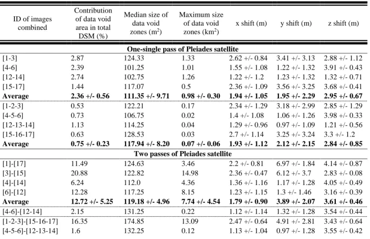
Table 2 examines a subset of DSMs out of the 150 calculations, chosen to result from the combination of images acquired in one single pass of the satellite, and from two passes at different times. Besides, all selected images come from Tri-Stereo acquisitions. All combinations possible with these constraints are presented, in effect resulting in stereo, tri-stereo, multi-stereo, and multi-tri-stereo cases. The robustness of the calculated DSMs is estimated through the relative extent of the total area with no recovered topographic points, as through the median and largest size of the zones with no data in the DSM. The accuracy of the calculated DSMs is estimated through the positioning difference between the absolute field GCPs and the equivalent calculated points.
With images acquired in one-single pass of the Pleiades satellite, the Tri-Stereo calculations provide systematically a more robust DSM than do the Stereo calculations: the total unresolved area is ~ three times smaller in Tri-Stereo calculations compared to Stereo results. Besides, while the median size of the unresolved zones is similar in both cases, the largest size of the unconstrained zones are much smaller in the Tri-Stereo case, by more than an order of magnitude.
By contrast, the accuracy of the DSMs is similar whether calculations are done in Stereo or Tri-Stereo. Whatever the calculation, the positioning is not better than about 2 m in the horizontal plane (in some cases up to 3-4 m and possibly more as uncertainties are large in a few cases), and about 3 m in the vertical dimension (up to 4 m in some cases).
Table 2: Influence of the number of Pleiades Images and sensor passes on the robustness and accuracy of the calculated DSMs. Images ID are from Table 1. All images used below come from Tri-Stereo acquisitions (not corrected with GCPs). Brackets indicate images acquired in one single pass. The data void area (area with no recovered topography) is presented as percentage of the total DSM surface, and with the maximum and median sizes of the zones with no data. The x, y and z shifts are calculated as described in text. Average values are provided for subsets including more than 2 combinations with a same number of images
ID of images combined Contribution of data void area in total DSM (%) Median size of data void zones (m2) Maximum size of data void zones (km2)
x shift (m) y shift (m) z shift (m)
One-single pass of Pleiades satellite
[1-3] 2.87 124.33 1.33 2.62 +/- 0.84 3.41 +/- 3.13 2.88 +/- 1.12 [4-6] 2.39 101.25 1.01 1.55 +/- 1.08 1.22 +/- 1.32 3.91 +/- 0.43 [12-14] 2.74 102.75 1.26 1.22 +/- 1.2 1.23 +/- 1.32 1.32 +/- 0.71 [15-17] 1.44 117.07 0.5 2.36 +/- 1.09 3.56 +/- 3.25 3.68 +/- 0.41 Average 2.36 +/- 0.56 111.35 +/- 9.71 0.98 +/- 0.30 1.94 +/- 1.05 1.95 +/- 2.29 2.95 +/- 0.67 [1-2-3] 0.53 122.21 0.17 2.34 +/- 1.29 3.18 +/- 2.99 2.85 +/- 1.29 [4-5-6] 0.73 106.75 0.02 1.4 +/- 1.08 1.06 +/- 1.26 3.98 +/- 0.33 [12-13-14] 1.13 114.25 0.04 1.29 +/- 0.96 0.97 +/- 1.09 1.21 +/- 0.56 [15-16-17] 0.63 128.53 0.03 2.7 +/- 1.14 3.25 +/- 3.24 3.3 +/- 1.2 Average 0.75 +/- 0.23 117.94 +/- 8.20 0.07 +/- 0.06 1.93 +/- 1.12 2.12 +/- 2.15 2.84 +/- 0.85 Two passes of Pleiades satellite
[1]-[17] 11.49 124.63 3.46 2.2 +/- 0.81 6.97 +/- 1.84 4.14 +/- 0.87 [3]-[15] 20.88 122.82 14.98 2.36 +/- 0.47 6.12 +/- 3.7 2.83 +/- 0.08 [4]-[14] 6.24 112.0 4.36 1.36 +/- 1.16 1.17 +/- 1.28 4.05 +/- 0.49 [6]-[12] 12.28 117.25 8.15 1.23 +/- 1.15 1.3 +/- 1.46 3.16 +/- 0.39 Average 12.72 +/- 5.25 119.18 +/- 4.96 7.74 +/- 4.54 1.79 +/- 0.90 3.89 +/- 2.07 3.61 +/- 0.46 [4-6]-[12-14] 2.15 131.25 0.22 1.12 +/- 1.14 1.32 +/- 1.28 3.54 +/- 0.44 [1-2-3]-[15-16-17] 16.35 174.85 13.09 2.47 +/- 0.64 4.91 +/- 2.81 3.43 +/- 0.64 [4-5-6]-[12-13-14] 1.6 132.25 0.12 1.13 +/- 1.04 0.97 +/- 1.28 3.55 +/- 0.42
Combining images acquired in two different satellite passes decreases overall the robustness of the calculated DSMs. The total unresolved area becomes about 7 times larger than in the previous single-pass cases, while the largest zones with no recovered data reach significant extents, up to ~12 times larger than in single-pass cases. Only the median size of the unresolved zones remains similar to that found in the previous single-pass cases, in the order of 100-150 m2.
By contrast, combining images from different satellite passes does not alter generally the accuracy of the DSMs: the horizontal positioning remains of about 2 m (yet in some cases up to 6-7 m), while the vertical positioning is about 3 m (up to 4 m in some cases). Example of visual results on Figure 7 confirms the conclusions drawn from Table 2.
When the image acquisition time is considered, we observe that the DSMs with the largest proportions of unresolved areas are those resulting from the combination of images acquired at more than 1.5 months interval. Conversely, in all cases, the combination of images acquired at time intervals less than 3 weeks provide better constrained DSMs.
The large proportions of unresolved areas in the DSMs can result from two factors, that may actually combine: (1) The difference in the acquisition time makes that sun shadows are different on the images, and likely longer on the images acquired at a time closer from the winter solstice. It is possible that these long shadows mask the ground topography locally and hence hamper its measurement at such local spots; (2) One may also suggest that the matching algorithm used in Micmac fails to identify tie points in some of the image pairs, for different reasons possibly including sun shadows.
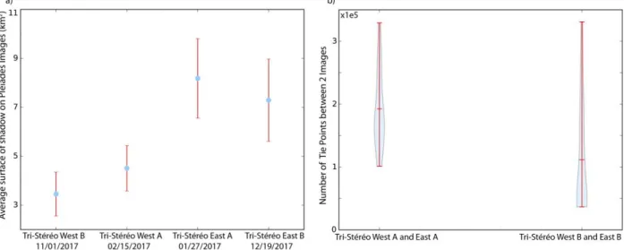
To examine the first hypothesis, we have measured the proportion of shadows in the four Tri-stereos whose images are used in Table 2. Shadow is considered as a radiometric black value in the range 0-15. We remind that there is no building, vegetation or water in the target zone, what ensures that the black zones are sun shadows. Figure 8a shows that the proportion of shadows is indeed important in the images, from about 3 to 8 km2 (2% and 4% from total surface).
It also depends on the acquisition time, since images acquired at the winter climax (Tri-stereo East B and East A, Table 1) have 2-3 times more shadow areas than images acquired earlier or later in the winter (Tri-stereo West B and West A). Therefore, the first hypothesis likely explains, at least partly, the large amounts of unresolved areas in the DSMs when images from markedly different times in the winter season are combined.
To examine the second hypothesis, we have determined the total number of Tie Points in the two double Tri-Stereos combinations (Figure 8b). That total number is the sum of the Tie Point amounts in each image pair calculation. We find that the number of Tie Points is twice lower in the DSM calculated from the two Tri-Stereos most distant in time (~1.5
Figure 7: From left to rightL Example of reconstructed DSMs, when using 2 and 3 images on one-single pass of the Pleiades satellite, and 2 and 6 images with two passes of the satellite, respectively. Percentages in brackets indicate the uncovered surface from total surface.
months interval) than in the DSM derived from triplets acquired at closer times. Therefore, long time delays between images seem to hamper the Tie Point identification through the Micmac SIFT procedure. This can be related to the greater and more heterogeneous extent of the sun shadows, and/or to other reasons. We explore these reasons below.
5.2 Analysis of the 150 DSMs
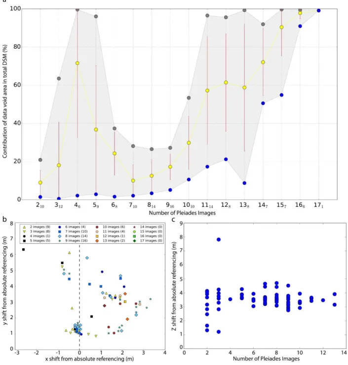
Figure 9 presents the robustness and the accuracy of the 150 calculated DSMs, here again expressed as the relative extent of the total unresolved area and the relative positioning of the calculated points with respect to the field GCPs, respectively. Here the DSMs have been calculated from the combination of a variable number of images, from 2 to 17, having different roll and pitch angles, and arising from a different number of Pleiades satellite passes. Figure 9a examines the mean (in yellow) relative extent of the unresolved areas as a function of the number of images used in the calculations (whose number is indicated). The DSMs with the lowest and the largest unresolved areas are indicated in blue and gray, respectively. Figure 9b presents the horizontal positioning with color codes indicating the number of images used in the DSM calculations, while Figure 9c presents the accuracy of the vertical positioning as a function of the number of images. Note that the template matching approach revealed poor correlation coefficients in some combination cases, which resulted in an inability to estimate the x, y and z shifts; these combinations are thus lacking in Figures 9b-c.
Figure 9a reveals a disorganized pattern. The unresolved zones occupy on average 10 to 20% of the site surface when 2 to 3 images are combined. Yet their relative importance fluctuates between insignificant to dramatic values greater than 60%. When 1 or 2 more images are included in the calculations, the importance of the unresolved areas increases abruptly and dramatically, reaching average surfaces more than half the total area, and up to the entire surface of the site. Then, adding 1 to 4 more images abruptly and markedly decreases the relative importance of the unresolved areas: those now occupy on average 10-20% of the surface site, and no more than 30-40%. Adding more images dramatically worsens again the DSMs, as most of them now have more than 60% of their surface being unresolved. The inability of the calculations to measure the topography is actually impressive, as some of the combinations with more than 10 images result to have no data at all. The fluctuations of the results are actually so large that, for a similar number of combined images, one can obtain a robustly constrained DSM with hardly a few percents of data voids (at least for combinations including up to 9 images), or, a totally unconstrained DSM with hardly a few percents of resolved topographic points.
As we showed before, the number of Tie Points identified in each image pair is critical in determining the robustness of the related DSM. The disorganized pattern revealed in Figure 9a might thus well result from the variability of the Tie Point density from one image pair to another. Figure 10 shows the distribution of the number of Tie Points identified in all image pairs built from one or other of the 17 images. On the graph the images are represented with their ID (from Table 1). Figure 10 shows that the amount of Tie Points significantly drops down when one or other of the images # 7 to 11 are included in the calculations, that is when one or other of the 5 Mono images are included in the DSM calculations. One likely reason is that the 5 Mono images have been acquired in the summer time or near time (between August and early October), and hence, at a long-time interval from the other Tri-Stereo images. When two images are separated by such long-time delays, they hold different sun shadows, and these differences hamper the Tie Point identification between them. The resulting low densities of Tie Points in turn produce weakly constrained DSMs, as likely some of those observed in Figure 9a. Yet, as we showed before, that the combined images were, or not, acquired during the same satellite pass also has a strong impact on the DSM robustness. Figure 9a does not discriminate the combinations as a function of the number of satellite passes. Therefore, we cannot assess the importance of this factor in the disorganized pattern of Figure 9a. More work needs to be done to address this issue.
Finally, Figure 9b shows that the number of images used in the DSM calculations does not have any clear impact on the accuracy of the horizontal positioning: whatever the number of images combined, the topographic data points are located with an uncertainty of ~1 to 3.5 m in the East direction. In the north direction, the uncertainty on positioning is also generally between ~1 and 3.5 m, but it can be larger, up to ~6 m, when less than 10 images are combined. Regarding the elevation accuracy of the DSMs (Figure 9c), it is stable, around 3-4 m, whatever the number of Pleiades images used in the calculations. Combining more than 3 images decreases the range of uncertainty fluctuations, however, but maintains the vertical uncertainty around 3-4 m, a greater value than it is found in a few calculations with 2 or 3 images. The number of combinations in general decreases with the increase of the number of images, so it is delicate to conclude that the fluctuations decrease.
Figure 8: (a) average area of shadow in each Tri-Stereo Acquisition; (b) Number of Tie Points in the two double Tri-Stereos combinations. The blue curve shows the distribution of the Tie Point number among the image pairs, while the average, minimum and maximum values are indicated in red.
Figure 9: (a) Relative extent of the unresolved areas in the 150 DSMs as a function of the number of Pleiades images used in the DSM calculations. The number of calculations is indicated as subscript. Blue, yellow and gray dots are the minimum, average (with associated standard deviation in red) and maximum extent of the unresolved areas, respectively. (b) Errors on the x and y localizations in the 150 DSMs. Colors and symbols discriminate the number of Pleiades Images used to generate the DSMs (number of combinations indicated in brackets). (c) Error on elevation in the 150 DSMs as a function of the number of Pleiades images used in the DSM calculations
6. CONCLUSION
In a desert target site with complex topography, we have conducted a multi-stereo Pléiades analysis dedicated to examine which Pleiades acquisition configuration best recovers the topography at high-resolution. We have reconstructed 150 DSMs over the studied area by using different combinations of 2 to 17 Pleiades images. By analyzing these DSMs and comparing their measures with 12 Ground Control Points we acquired on the field, we obtained the following principal results:
(1) Tri-Stereo DSMs are systematically more robust (i.e., having topography resolved in a larger area) than Stereo DSMs when the combined images were acquired at a same or a close time period (< ~3 weeks). The three images need not be acquired in a single satellite pass. By contrast, if the combined images were acquired with a significant time delay, Tri-Stereo does not necessarily increase the robustness of the DSMs.
(2) More generally, combining images acquired with significant time delays can dramatically decrease the robustness of the resulting DSMs (Figure 9a and Table 2). Conversely, performing Multi-Stereo (i.e., with more than 3 images) with images acquired in similar, though not exact same times, can improve the DSM robustness (Figure 9a, see cases 7 & 8). (3) The accurate determination of tie points is critical for robust DSM reconstruction. The SIFT-based procedure reveals to fail dramatically in identifying tie points as soon as moderate time delays on the order of 1-2 months separate the image acquisitions. Other, more efficient approaches for tie point identification thus seem to be needed to overcome this significant limitation.
(4) Regardless of their acquisition time, combining an increased number of images improves the accuracy of the positioning of the DSMs (provided that those could be calculated with enough topographic data).
In the future, we will extend our study with the calculation of DSMs, using another tie points detector than SIFT which is less sensitive to changes in the pixel intensities. We will also efficiently study the impact of the number of passages of the Pleiades Satellite, on the DSM reconstruction.
7. REFERENCES
1. Stewart, N. et al. “3D_Fault_Offsets,” a Matlab Code to Automatically Measure Lateral and Vertical Fault Offsets in Topographic Data: Application to San Andreas, Owens Valley, and Hope Faults. J. Geophys. Res. Solid Earth 123, 815–835 (2018).
Figure 10: Number of Tie Points generated in all image pairs with with one or other of the reference images listed in horizontal axis with their ID (from Table 1). The yellow curve shows the distribution of the Tie Point number among the image pairs, while the average, minimum and maximum values are indicated in red.
2. Grosse, P., van Wyk de Vries, B., Euillades, P. A., Kervyn, M. & Petrinovic, I. A. Systematic morphometric characterization of volcanic edifices using digital elevation models. Geomorphology 136, 114–131 (2012).
3. van Westen, C. J. & Lulie Getahun, F. Analyzing the evolution of the Tessina landslide using aerial photographs and digital elevation models. Geomorphology 54, 77–89 (2003).
4. A new method for the determination of flow directions and upslope areas in grid digital elevation models. Water
Resour. Res. 33, 309–319
5. Sanyal, J. & Roychowdhury, K. Tracking the relationship between changing skyline and population growth of an Indian megacity using earth observation technology. Geocarto Int. 32, 1421–1435 (2017).
6. Simons, M., Fialko, Y. & Rivera, L. Coseismic Deformation from the 1999 Mw 7.1 Hector Mine, California, Earthquake as Inferred from InSAR and GPS Observations. Bull. Seismol. Soc. Am. 92, 1390–1402 (2002).
7. Delouis, B., Nocquet, J.-M. & Vallée, M. Slip distribution of the February 27, 2010 Mw = 8.8 Maule Earthquake, central Chile, from static and high-rate GPS, InSAR, and broadband teleseismic data. Geophys. Res. Lett. 37, 8. Bawden, G. W., Thatcher, W., Stein, R. S., Hudnut, K. W. & Peltzer, G. Tectonic contraction across Los Angeles
after removal of groundwater pumping effects. Nature 412, 812 (2001).
9. Sidjak, R. W. Glacier mapping of the Illecillewaet icefield, British Columbia, Canada, using Landsat TM and digital elevation data. Int. J. Remote Sens. 20, 273–284 (1999).
10. Yamazaki, F. & Liu, W. Remote Sensing Technologies for Post-Earthquake damage assessment: a case study on the 2016 Kunamoto Earthquake. 14 (2016).
11. Rabus, B., Eineder, M., Roth, A. & Bamler, R. The shuttle radar topography mission—a new class of digital elevation models acquired by spaceborne radar. ISPRS J. Photogramm. Remote Sens. 57, 241–262 (2003).
12. Farr, T. G. et al. The shuttle radar topography mission. Rev. Geophys. 45, (2007).
13. Oh, J. & Lee, C. Automated bias-compensation of rational polynomial coefficients of high resolution satellite imagery based on topographic maps. ISPRS J. Photogramm. Remote Sens. 100, 14–22 (2015).
14. Guidi, G. et al. A multi-resolution methodology for the 3D modeling of large and complex archeological areas. Int.
J. Archit. Comput. 7, 39–55 (2009).
15. Myers, R. & Aydin, A. The evolution of faults formed by shearing across joint zones in sandstone. J. Struct. Geol.
16. Joussineau, G. de, Mutlu, O., Aydin, A. & Pollard, D. D. Characterization of strike-slip fault–splay relationships in sandstone. J. Struct. Geol. 29, 1831–1842 (2007).
17. de Joussineau, G. & Aydin, A. The evolution of the damage zone with fault growth in sandstone and its multiscale characteristics. J. Geophys. Res. Solid Earth 112, B12401 (2007).
18. Rupnik, E., Daakir, M. & Deseilligny, M. P. MicMac–a free, open-source solution for photogrammetry. Open
Geospatial Data Softw. Stand. 2, 14 (2017).
19. Rupnik, E., Deseillignya, M. P., Delorme, A. & Klinger, Y. Refined satellite image orientation in the free open-source photogrammetric tools apero/micmac. ISPRS Ann. Photogramm. Remote Sens. Spat. Inf. Sci. 3, (2016).
20. Roy, S. & Cox, I. J. A maximum-flow formulation of the n-camera stereo correspondence problem. in Computer
Vision, 1998. Sixth International Conference on 492–499 (IEEE, 1998).
21. Lowe, D. G. Distinctive image features from scale-invariant keypoints. Int. J. Comput. Vis. 60, 91–110 (2004). 22. Li, Q., Wang, G., Liu, J. & Chen, S. Robust scale-invariant feature matching for remote sensing image registration.
IEEE Geosci. Remote Sens. Lett. 6, 287–291 (2009).
23. Hartley, R. & Zisserman, A. Multiple view geometry in computer vision. (Cambridge university press, 2003). 24. Pierrot-Deseilligny, M. & Paparoditis, N. A multiresolution and optimization-based image matching approach: An
application to surface reconstruction from SPOT5-HRS stereo imagery. Arch. Photogramm. Remote Sens. Spat. Inf.
Sci. 36, (2006).