HAL Id: hal-01806683
https://hal.archives-ouvertes.fr/hal-01806683
Submitted on 27 Oct 2020
HAL is a multi-disciplinary open access
archive for the deposit and dissemination of
sci-entific research documents, whether they are
pub-lished or not. The documents may come from
teaching and research institutions in France or
abroad, or from public or private research centers.
L’archive ouverte pluridisciplinaire HAL, est
destinée au dépôt et à la diffusion de documents
scientifiques de niveau recherche, publiés ou non,
émanant des établissements d’enseignement et de
recherche français ou étrangers, des laboratoires
publics ou privés.
Earth system models using atmospheric potential
oxygen and ocean color data
C. Nevison, M. Manizza, R. Keeling, M. Kahru, L. Bopp, J. Dunne, J.
Tiputra, T. Ilyina, B. Mitchell
To cite this version:
C. Nevison, M. Manizza, R. Keeling, M. Kahru, L. Bopp, et al.. Evaluating the ocean
biogeochem-ical components of Earth system models using atmospheric potential oxygen and ocean color data.
Biogeosciences, European Geosciences Union, 2015, 12 (1), pp.193 - 208. �10.5194/bg-12-193-2015�.
�hal-01806683�
www.biogeosciences.net/12/193/2015/ doi:10.5194/bg-12-193-2015
© Author(s) 2015. CC Attribution 3.0 License.
Evaluating the ocean biogeochemical components of Earth system
models using atmospheric potential oxygen and ocean color data
C. D. Nevison1, M. Manizza2, R. F. Keeling2, M. Kahru2, L. Bopp3, J. Dunne4, J. Tiputra5, T. Ilyina6, and B. G. Mitchell2
1University of Colorado, Boulder, Institute for Arctic and Alpine Research, Boulder, Colorado, USA 2Scripps Institution of Oceanography, La Jolla, California, USA
3IPSL/LSCE, UMR8212, CNRS-CEA-UVSQ, Gif sur Yvette, France
4National Oceanic and Atmospheric Administration/Geophysical Fluid Dynamics Laboratory, Princeton, New Jersey, USA 5Uni Climate, Uni Research and Bjerknes Centre for Climate Research, Bergen, Norway
6Max Planck Institute for Meteorology, Hamburg, Germany
Correspondence to: C. D. Nevison (cynthia.nevison@colorado.edu)
Received: 1 April 2014 – Published in Biogeosciences Discuss.: 11 June 2014
Revised: 28 October 2014 – Accepted: 22 November 2014 – Published: 12 January 2015
Abstract. The observed seasonal cycles in atmospheric
po-tential oxygen (APO) at a range of mid- to high-latitude sur-face monitoring sites are compared to those inferred from the output of six Earth system models (ESMs) participat-ing in the fifth phase of the Coupled Model Intercompar-ison Project phase 5 (CMIP5). The simulated air–sea O2
fluxes are translated into APO seasonal cycles using a matrix method that takes into account atmospheric transport model (ATM) uncertainty among 13 different ATMs. Three of the ocean biogeochemistry models tested are able to reproduce the observed APO cycles at most sites, to within the large TransCom3-era ATM uncertainty used here, while the other three generally are not. Net primary production (NPP) and net community production (NCP), as estimated from satellite ocean color data, provide additional constraints, albeit more with respect to the seasonal phasing of ocean model produc-tivity than overall magnitude. The present analysis suggests that, of the tested ocean biogeochemistry models, the com-munity ecosystem model (CESM) and the Geophysical Fluid Dynamics Laboratory (GFDL) ESM2M are best able to cap-ture the observed APO seasonal cycle at both northern and southern hemispheric sites. In most models, discrepancies with observed APO can be attributed to the underestimation of NPP, deep ventilation or both in the northern oceans.
1 Introduction
Ocean physical and biogeochemical processes have profound influences on Earth’s climate. Phytoplankton in the sunlit part of the ocean convert carbon from inorganic to organic form via photosynthesis, thereby establishing the base of the ocean food chain. Primary production and subsequent export of organic carbon from the mixed layer (export production, EP) and remineralization at depth are key components of the so-called biological pump, which regulates the partition of carbon between the ocean and atmosphere (Gruber and Sarmiento, 2002; Boyd and Doney, 2003).
Net community production (NCP) and the related process of EP are also important for understanding the distribution of dissolved O2within the ocean and the flux of O2(FO2)at the
air–sea interface. NCP is defined here as the net amount of organic carbon fixed through photosynthesis over the depth of the mixed layer after accounting for grazing and both au-totrophic and heterotrophic respiration. NCP is closely linked to FO2, since each mole of photosynthetically fixed carbon
that persists beyond the timescale of air–sea exchange (2– 3 weeks) leaves a stoichiometric amount of O2available for
release to the atmosphere. This release of O2 to the
atmo-sphere in association with NCP occurs mainly in the spring and summer at extratropical latitudes (Keeling et al., 1993). EP more or less balances NCP when averaged over a full year or if the upper ocean is in a long-term steady state and
advec-tive fluxes are zero (Laws et al., 2000). The exported carbon subsequently is respired in the subsurface ocean, leading to O2depletion at depth. O2is replenished by absorption from
the atmosphere when deep waters mix back to the surface in fall and winter. Deep ventilation and NCP thus are distinct processes that are largely separate in time and space but are both closely linked to the biological pump that draws car-bon out of surface waters and is critical for ocean uptake of atmospheric CO2.
To explore the impacts of future climate change on Earth’s climate and ecosystems, the Coupled Model Intercomparison Project phase 5 (CMIP5) relies on three-dimensional numeri-cal Earth system models (ESMs), which incorporate descrip-tions of biogeochemical impacts of land and marine biota. Projections of future atmospheric CO2levels and associated
climate warming in the CMIP5 depend not only on fossil fuel use projections but also on assumptions about uptake and storage of carbon by the land and ocean. The oceans have absorbed approximately one-third of the anthropogenic car-bon released to the atmosphere since the beginning of the industrial era (Khatiwala et al., 2009), but this fractional rate of uptake is unlikely to continue in the future as the buffering capacity of surface waters declines and the export of carbon from the surface to the deep ocean fails to keep pace with anthropogenic fossil fuel combustion (Arora et al., 2013). Changes in ventilation of abyssal deepwater are an additional possible consequence of future climate forcing that current models may or may not be able to predict accurately (Sig-man et al., 2010).
Recent studies have tested the present-day skill of the ocean components of ESMs and some have also examined future projections (Schneider et al., 2008; Steinacher et al., 2010, Bopp et al., 2013; Anav et al., 2013). These evaluations have compared model output to both hydrographic measure-ments and remotely sensed ocean color products, most com-monly net primary production (NPP). The models predict spatial–annual patterns in NPP that reproduce some of the main features seen in satellite data, but differ over a fac-tor of 2 in NPP magnitude. Some evaluations have exam-ined seasonal variability and have found that ocean models tend to underestimate observed NPP at high latitudes (pole-ward of 44◦) in the Northern Hemisphere and overestimate it in the Southern Hemisphere. The models also fail to cap-ture the timing of the observed high-latitude peak in NPP in both hemispheres, with predictions that are often 1–2 months earlier than observations (Anav et al., 2013; Henson et al., 2013). However, ocean color-derived NPP values are uncer-tain, especially in the Southern Ocean, reducing confidence in the observed constraints.
Many biogeochemical processes that are expected to oc-cur in the future, such as responses to warming and stratifi-cation, are also highly relevant on seasonal timescales (Keel-ing et al., 2010; Anav et al., 2013). Thus, challeng(Keel-ing models against known seasonal variations can aid in the development of credible predictions of future changes. Here, we evaluate
six ESMs used in the CMIP5 against two cross-cutting met-rics, which test the models’ ability to account for changes in ocean biogeochemistry on seasonal time frames. This work is intended primarily as a demonstration of method using an available subset of the CMIP5 ESMs rather than as a compre-hensive evaluation of all the CMIP5 models. The first metric is based on satellite-derived estimates of ocean color, focus-ing on NPP and NCP. The second metric is based on the sea-sonal cycles in atmospheric potential oxygen (APO), an at-mospheric tracer that varies seasonally mainly due to air–sea exchanges of O2(Stephens et al., 1998; Manning and
Keel-ing, 2006).
EP is the ocean color-derived flux most relevant to the bi-ological pump, but cannot be directly observed by remote sensing. It is derived by a combination of remote measure-ments and poorly constrained models, which inherently in-creases its uncertainty (Schneider et al., 2008; Nevison et al., 2012a). The quantity actually observed from space is spectral top-of-the-atmosphere radiance, which is used to estimate chlorophyll (or another proxy of phytoplankton biomass); chlorophyll and other variables such as photosynthetic radia-tion are used to estimate NPP and, finally, NPP is used to es-timate EP. The first step, estimation of chlorophyll, is known to have significant bias (underestimation by ∼ 2–3 times) in the Southern Ocean which is transferred to higher level prod-ucts. We correct for that bias by using algorithms tuned to Southern Ocean data sets blended with more or less standard products elsewhere (Mitchell and Kahru, 2009; Kahru and Mitchell, 2010). While our satellite estimates of EP are im-proved, they are still subject to high uncertainty.
Observed seasonal cycles in APO provide a new bench-mark for the ocean biogeochemistry model components of ESMs. They offer evaluation metrics complementary to ocean color products by providing additional information on deep ventilation processes unavailable from satellite data alone. The main drawback of APO seasonal cycles is that atmospheric transport models (ATMs) are needed to trans-late ocean model air–sea O2fluxes into a seasonal APO
sig-nal, which inevitably introduces uncertainty (Stephens et al., 1998; Nevison et al., 2012a). A first attempt has been made to use APO seasonal cycles to evaluate ocean-only marine bio-geochemistry models (Naegler et al., 2007), but the models in that study implemented a simplified parameterization of the biological processes affecting O2and CO2air–sea fluxes and
were considerably less advanced than the current ecosystem dynamics and biogeochemical components used in state-of-the-art ESMs. Further, while Naegler et al. (2007) asserted that the uncertainty introduced by ATMs was too large to pro-vide a strong constraint on ocean model fluxes, their study re-lied on only two ATMs. Here, we translate the model air–sea fluxes into APO signals using a wider range of ATMs and show that, in many cases, the discrepancies between mod-eled and observed APO seasonal cycles transcend ATM un-certainty.
2 Methods
2.1 Ocean biogeochemistry models
The CMIP5 models analyzed in this study include the Geo-physical Fluid Dynamics Laboratory (GFDL) ESMs (depth-based ESM2M and density-(depth-based ESM2G vertical oceans; Dunne et al., 2012) from Princeton, New Jersey; the In-stitut Pierre Simon Laplace Coupled Model 5 in its low-resolution version (IPSL-CM5A-LR, hereafter referred to as IPSL) model from Paris, France; the community ecosystem model (CESM) from the National Center for Atmospheric Research in Boulder, CO; the Max Planck Institute for Mete-orology (MPIM) ESM, version MPI-ESM-LR, from Ham-burg, Germany; and the Norwegian ESM (NorESM1-ME, hereafter referred to as NorESM1). The ocean biogeochemi-cal models embedded in the respective ESMs are represented by the Tracers of Phytoplankton with Allometric Zooplank-ton (TOPAZ) (GFDL) (Dunne et al., 2013), Pelagic Inter-action Scheme for Carbon and Ecosystem Studies (PISCES) (IPSL) (Aumont and Bopp, 2006), biogeochemical elemental cycling (BEC) (CESM) (Moore et al., 2002, 2004, 2013), and Hamburg Ocean Carbon Cycle (HAMOCC) (MPIM) (Ilyina et al., 2013). NorESM1 uses a variant of HAMOCC, adapted to a sigma-coordinate ocean circulation model (Tjiputra et al., 2013).
The six ESMs differ in their physical components and im-plement ocean biogeochemical schemes that vary in their specifics, but have many common features. All include ex-plicit representations of upper ecosystem dynamics that dis-tinguish at least one phytoplankton group and one size class of zooplankton. Four of the models (CESM, both GFDL vari-ants and IPSL) divide phytoplankton further into at least two size classes: large (micro) and small (nano + pico). GFDL and CESM also explicitly model diazotrophs. Phytoplankton growth rates in all models are co-limited by light, temper-ature and nutrient (N, P, Si, Fe) availability. Carbon export flux is closely linked to ecosystem structure and dynamics, with higher sinking rates assumed for large phytoplankton, representing, e.g., diatoms.
For each model, the following output fields were obtained for the CMIP5 standard historical simulation, which is driven by prescribed atmospheric CO2 from 1850 to 2005:
car-bon export flux at 100 m depth (EP100), vertically integrated
NPP, net air–sea O2 and CO2 fluxes, net surface heat flux
(Q), and sea surface salinity and temperature (SST). Many of these fields were available through public web interfaces, but some variables, particularly Q, required assistance from the individual modeling groups, which effectively limited the study to the six models listed above. The EP100 and NPP
fields were compared directly to the corresponding satel-lite ocean color products. The remaining five output fields were used in the estimation of APO time series, with the final three fields used to estimate air–sea N2 fluxes based
on the Q(dS/dT )N2/Cpequation (Keeling et al., 1993;
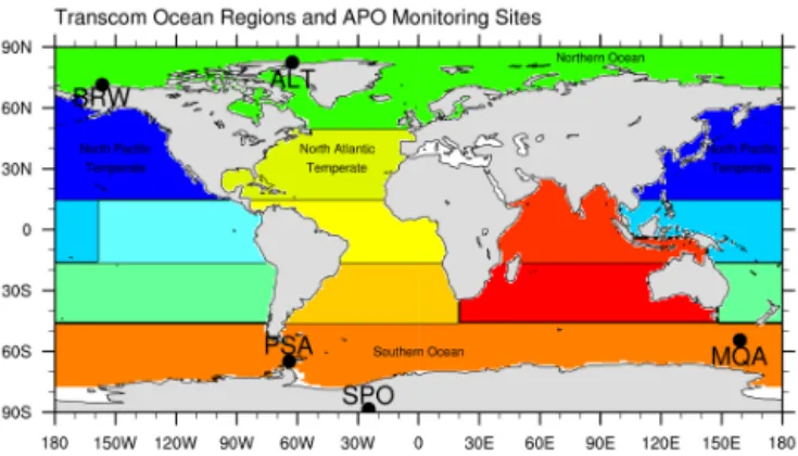
Man-Figure 1. TransCom3 Level 2 ocean regions used in the matrix-based atmospheric transport method. Locations of the five APO monitoring sites featured in Fig. 2 are superimposed.
izza et al., 2012) with modifications from Jin et al. (2007). In this equation, Q is heat flux, (dS/dT )N2 is the
tempera-ture derivative of the N2solubility coefficient and Cpis the
heat capacity of sea water. The resulting N2fluxes, together
with the prognostic O2and CO2air–sea fluxes, were used as
described below to force atmospheric transport model sim-ulations to compute atmospheric time series of APO (Nae-gler et al., 2007; Nevison et al., 2008; 2012a). Since all the ocean models operated on an irregular, off-polar grid with two-dimensional latitude and longitude coordinates, these were first interpolated to a regular 1◦×1◦ latitude– longitude grid using climate data operator (CDO) freeware (https://code.zmaw.de/projects/cdo). The climate data opera-tor interpolation was not mass conservative, but resulted in global O2flux differences generally of less than 1 %. An
ex-ception was the CESM, whose output was converted conser-vatively to a regular grid using a CESM-specific mapping file.
2.2 Atmospheric transport model simulations 2.2.1 Matrix method
A matrix method was used to translate the ocean model air–sea O2, N2 and CO2 fluxes into corresponding annual
mean cycles in atmospheric potential oxygen (APO). The method was based on the pulse-response functions from the TransCom3 Level 2 (T3L2) ATM intercomparison. Each of the 13 ATMs that participated in T3L2 conducted for-ward simulations in which a uniformly distributed CO2flux,
normalized to 1 PgC yr−1, was released from each of 11
ocean regions (Fig. 1) for each of 12 emission months, i.e., January–December, allowed to decay for 35 months, using an annually repeating cycle of meteorology that was model specific for each ATM, and sampled every month at a range of surface monitoring sites (Gurney et al., 2003; 2004). The APO code was developed from an earlier pulse-response ma-trix code, which has been described in detail in Nevison et
al. (2012b), that translates terrestrial net ecosystem exchange (NEE) fluxes of carbon into the corresponding annual mean cycles in atmospheric CO2. The matrix method is
consid-erably faster than a full forward ATM simulation, allowing annual mean cycles in APO from 13 different ATMs to be computed in seconds, rather than the days or weeks required for a single forward simulation.
The pulse-response matrix code was applied separately to the O2, N2and oceanic CO2fluxes from the last 12 years of
the historical simulations, spanning 1994–2005, converting from carbon to oxygen or nitrogen units where appropriate, to create three separate time series of atmospheric O2, N2
and CO2as mole fraction anomalies (µmol mol−1)on a H2
O-free basis, where the O2and N2anomalies are computed as
though O2and N2were trace gases, similar to CO2. These
were combined to calculate a 9-year time series in APO in per meg units, spanning 1997 to 2005, according to Eq. (1) (Stephens et al., 1998): APO = 1 XO2 (O2) − 1 XN2 (N2) + 1.1 XO2 (CO2), (1)
where XO2 and XN2 are the dry air mole fractions of O2
and N2 in H2O-free air, treated here as constants (0.2094
and 0.7808, respectively). The mean seasonal cycle was com-puted by detrending the time series with a third-order polyno-mial and then taking the average of the detrended data for all Januaries, Februaries, etc. The matrix method involves cal-culating separately the components of APO at each measure-ment site arising from fluxes from each ocean region. These components are then summed to compute the net APO sig-nal. The model definition of APO in Eq. (1) ignores contribu-tions to APO from land biospheric exchanges at ratios other than 1 : 1 and fossil fuel burning, but these are very small in comparison to oceanic contributions on seasonal timescales (Manning and Keeling, 2006; Nevison et al., 2008).
2.2.2 Evaluation of matrix method based on APO TransCom
An evaluation exercise was conducted in which the APO pulse-response matrix code was forced by climatological O2
and N2fluxes from Garcia and Keeling (2001) and used to
compute the mean seasonal cycle in APO as described above using Eq. (1) (minus the oceanic CO2 term). The
matrix-based results were evaluated against the mean seasonal cy-cles from archived station output from the forward ATM sim-ulations of the APO TransCom Experiment, which also used the Garcia and Keeling O2 and N2 forcing fluxes (Blaine,
2005; Nevison et al., 2012b). This evaluation was conducted using a subset of 9 of the original 13 T3L2 ATMs that also participated in APO TransCom. For this subset, the matrix method performed well in relatively homogeneous regions like the Southern Ocean and at northern high-latitude sites like Barrow, Alaska (BRW) and Alert, Canada (ALT). It was less reliable in capturing the forward simulation cycle at sites
located within northern mid-latitude ocean regions, includ-ing Cold Bay, Alaska, and La Jolla, California, where the uniform distribution of fluxes assumed by T3L2 did not ac-curately capture the impact of strong heterogeneity in air–sea fluxes from these regions (Tables S1, S2 and Figs. S1, S2 in the Supplement). These same North Pacific stations are sub-ject to large uncertainty in full forward ATM simulations due to uncertainty in vertical mixing (Stephens et al., 1998; Bat-tle et al., 2006; Tohjima et al., 2012). We therefore focus in Sect. 3 on ALT, BRW and three Southern Ocean sites, in-cluding Macquarie Island (MQA), Palmer Station, Antarctica (PSA) and the South Pole (SPO) in our use of APO to eval-uate the ESM-simulated air–sea O2, N2and CO2fluxes. The
locations of these five sites with respect to the T3L2 ocean regions are shown in Fig. 1.
While the evaluation exercise indicates that the matrix method reproduces the shape and phase of the seasonal cy-cles with high reliability at the above sites, it tends to un-derestimate the seasonal amplitude by about 4–5 % at ALT and BRW and by 11–12 % at MQA and SPO and to slightly overestimate the amplitude at PSA. In applying the matrix code to the ESM oceanic fluxes, we therefore scaled up the estimated cycles by site and ATM-specific scaling factors ob-tained from the evaluation exercise (Tables S1, S2, Fig. S2). Since these scaling factors were only available for the sub-set of 9 of the 13 T3L2 ATMs that also participated in APO TransCom, we subsequently (Sect. 3.1) compare observa-tions alternatively to the scaled nine-model subset, or to all 13 unscaled models.
2.2.3 Component O2fluxes
The net air–sea O2 flux for each ESM can be divided into
three components, associated with NCP, deep ventilation and thermal processes (Nevison et al., 2012a):
FO2,total=FO2,NCP+FO2,vent+FO2,therm. (2)
These in turn can be used to force the matrix model and the resulting total APO cycle can be presented as the sum of component signals according to Eq. (3).
APO = APONCP+APOvent+APOtherm (3)
Here, the APOtherm term also includes the effects of N2
fluxes, as per the second right-hand term in Eq. (1). The at-mospheric signal due to oceanic CO2(last term in Eq. 1) is
not easily included in any of the component terms in Eq. (3) based on available ESM output, but in principle all three component processes may lead to changes in CO2fluxes as
well as O2fluxes. In practice, CO2has only a small influence
on the amplitude and phasing of APO in most of the ESMs and thus is ignored in the component analysis. An exception is the MPIM, in which the oceanic CO2signal has a peak–
trough seasonal amplitude of up to 5 ppm in the Southern Ocean that opposes the O2cycle, as noted previously (Anav
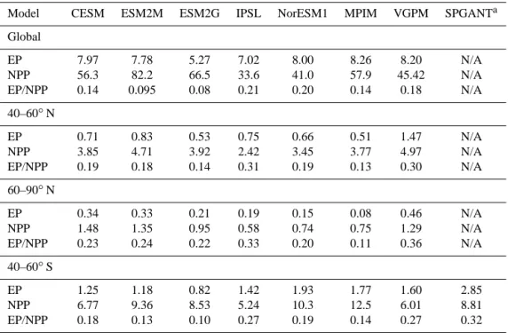
Table 1. Vertically integrated NPP, EP at 100 m (both in Pg C yr−1) and EP/PP for six CMIP5 models and two satellite products. Model CESM ESM2M ESM2G IPSL NorESM1 MPIM VGPM SPGANTa Global EP 7.97 7.78 5.27 7.02 8.00 8.26 8.20 N/A NPP 56.3 82.2 66.5 33.6 41.0 57.9 45.42 N/A EP/NPP 0.14 0.095 0.08 0.21 0.20 0.14 0.18 N/A 40–60◦N EP 0.71 0.83 0.53 0.75 0.66 0.51 1.47 N/A NPP 3.85 4.71 3.92 2.42 3.45 3.77 4.97 N/A EP/NPP 0.19 0.18 0.14 0.31 0.19 0.13 0.30 N/A 60–90◦N EP 0.34 0.33 0.21 0.19 0.15 0.08 0.46 N/A NPP 1.48 1.35 0.95 0.58 0.74 0.75 1.29 N/A EP/NPP 0.23 0.24 0.22 0.33 0.20 0.11 0.36 N/A 40–60◦S EP 1.25 1.18 0.82 1.42 1.93 1.77 1.60 2.85 NPP 6.77 9.36 8.53 5.24 10.3 12.5 6.01 8.81 EP/NPP 0.18 0.13 0.10 0.27 0.19 0.14 0.27 0.32 aSPGANT totals are only shown for the 40–60◦S band because the algorithm is optimized for the Southern Ocean but not well
validated in the Northern Hemisphere.
Among the terms in Eq. (2), FO2,total was provided
out-right by the ESMs and the thermal component FO2,therm
can be derived easily from standard ESM output follow-ing the approach described above for N2. The remaining
terms, FO2,NCP and FO2,vent are more challenging to
esti-mate from available ESM output. In Nevison et al. (2012a),
FO2,NCP was estimated from EP multiplied by a molar
ra-tio of 1.4 mol O2per mol C exported. The assumption that
FO2,NCP=1.4 EP was shown in Nevison et al. (2012a) to
yield reasonable results for EP derived from satellite data (and indeed was applied to the satellite data described be-low in Sect. 2.3), but this approach proved unsatisfactory for EP100 from the ESMs, especially in the Southern Ocean as
discussed further below, since it yielded an atmospheric sig-nal that was unreasonably small. The assumption also led to phasing uncertainties for some models (IPSL, NorESM1 and MPIM) that use finite sinking velocities for particulate organic carbon (as opposed to instantaneous vertical redis-tribution, as assumed, e.g., by CESM) with a resulting de-lay in EP100relative to NPP. Since the timing of FO2,NCPis
likely to be more closely related to NPP than EP100
(Nevi-son et al., 2012a), we estimated FO2,NCP from the ESMs
al-ternatively as 1.4 EP100 and 1.4 ef∗ NPP, where NPP is the
standard, vertically integrated ESM output variable and ef is the model-specific annual mean EP100/NPP ratio, integrated
over the 40–60◦N or 40–60◦S latitude band for northern and southern stations, respectively (Table 1).
Finally, FO2,ventin principle can be estimated as a residual
of the other three terms in Eq. (2). FO2,vent was estimated
with reasonable success at the northern hemispheric sites, but generally looked unreasonable in the Southern Ocean for most models, with the exception of the IPSL. The sig-nals were judged to be unreasonable on the basis of whether the APOvent term, if estimated as a residual from Eq. (3),
dominated the APONCP term in driving the springtime rise
in APO. In reality, the APONCP term must be primarily
re-sponsible for this rise (Keeling et al., 1993; Bender et al., 1996; Nevison et al., 2012a). We therefore do not attempt to explicitly resolve or present APOventsignals in the Southern
Hemisphere. While the problems with APOvent necessarily
imply a corresponding problem in one or both of the other component terms APONCP and APOtherm, as discussed
be-low, the shape of these latter terms is still informative and is less sensitive to the uncertainties inherent in the residually estimated APOventterm.
2.3 Satellite ocean color data
The primary output product of satellite ocean color mea-surements historically has been the concentration of chloro-phyll a (Chl), which is also the main input to most satellite-based ocean primary productivity models (Behrenfeld and Falkowski, 1997). However, the standard Chl product based on empirical band ratios of reflectances represents primar-ily the coefficient of total absorption of blue light and is inherently biased if the distributions of the optically active components deviate from the global mean (Lee et al., 2011; Siegel et al., 2005; Sauer et al., 2012). In the Southern Ocean
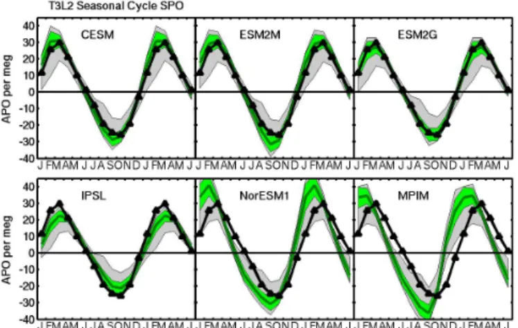
Figure 2a. Results of the pulse-response code forced by O2, N2and CO2 air–sea fluxes from six ESM ocean biogeochemistry model
components. The dark green line and light green window show the mean and standard deviation, respectively, of the nine ATMs par-ticipating in both T3L2 and APO TransCom. The amplitudes are scaled for each ATM and monitoring site based on the validation exercise described in Sect. 2.2.2 and illustrated in the Supplemen-tary material. The gray window shows the full range of responses from all 13 T3L2 ATMs, uncorrected based on the APO TransCom validation exercise. The heavy black line shows the observed APO mean annual cycle. (a) Results at South Pole, compared to SIO ob-servations.
the standard Chl algorithms underestimate in situ Chl by 2– 3 times (Mitchell and Kahru, 2009), whereas in the Arctic they overestimate it (Mitchell, 1992). These errors are di-rectly transferred into errors in estimates of NPP and EP.
For the Southern Hemisphere we used an empirical Chl al-gorithm (Scripps Photobiology) that was tuned to in situ Chl in the Southern Ocean and spatially blended with the stan-dard SeaWiFS OC4 algorithm (Kahru and Mitchell, 2010). The same blending scheme was applied when blending NPP between two versions of the Vertically Generalized Produc-tivity Model (VGPM) algorithm (Behrenfeld and Falkowski, 1997): the Southern Ocean version and the low-latitude ver-sion of Kahru et al. (2009). EP was calculated using a modi-fied version of the Laws (2004) model according to Nevison et al. (2012a). The mean annual cycles for Chl, NPP and EP were calculated for 1997–2009 using data derived from Sea-WiFS.
For the Northern Hemisphere we used NPP data calculated according to the standard VGPM using MODIS-Aqua Chl. NPP was downloaded from http://science.oregonstate.edu/ ocean.productivity. EP was calculated according to Dunne et al. (2005). The mean annual cycles for NPP and EP were calculated for 2002–2011 using monthly composites derived from MODIS-Aqua. While the Laws (2004) and Dunne et al. (2005) methods of deriving EP are not identical, they both estimate export efficiency as a function of sea surface tem-perature and NPP, are fitted to in situ data, and generally pro-duce similar estimates. In Nevison et al. (2012a) the Southern
Ocean EP derived with the Laws (2004) model was modified by constraining to the bulk nutrient budget estimated in the ocean inversion of Schlitzer (2002). That reduced the unreal-istically high export efficiency of the Laws (2004) model at cold temperatures and brought it into closer agreement with the Dunne et al. (2005) export efficiency.
Both the SPGANT and VGPM/OSU (Oregon State Uni-versity) satellite algorithms for NCP were converted to air– sea O2 fluxes using FO2,NCP=1.4 NCP, where 1.4 refers
to the molar ratio between O2 produced and carbon fixed
in photosynthesis. FO2,NCP was used to force the
pulse-response code to estimate the corresponding APO signal as-sociated with NCP as per Nevison et al. (2012a).
2.4 APO data
APO is a unique atmospheric tracer of ocean biogeochem-istry that is calculated by combining high precision O2 and
CO2data according to APO = O2+1.1CO2(Stephens et al.,
1998). By design, APO is mostly insensitive to exchanges with the land biosphere, which have a nearly fixed stoichiom-etry that produces compensating changes in O2and CO2. In
contrast, the exchanges of O2and CO2across the air–sea
in-terface are not strongly correlated, largely because variability in dissolved CO2is strongly damped by carbonate chemistry
in seawater on seasonal timescales. As a result, seasonal vari-ability in APO reflects changes in atmospheric oxygen occur-ring almost solely due to oceanic processes (Manning and Keeling, 2006).
Atmospheric O2 data, reported in terms of deviations in
the O2/N2ratio, were obtained from the Scripps Institution
of Oceanography (SIO) and Princeton University (PU) net-works. Data are available from the early to mid-1990s, de-pending on the station (Bender et al., 2005; Manning and Keeling, 2006). In Fig. 2, we use SIO data from SPO, PSA and ALT and PU data from MQA and BRW. Details of the station locations and time spans of data used to cal-culate the mean seasonal cycle are listed in Table S2 and shown in Fig. 1. For MQA (1997–2007) and BRW (1993– 2008), the time spans overlapped mostly but not perfectly with the CMIP5 model output (1994–2005) and the satellite data (1997–2009 for SPGANT, 2002–2011 for VGPM).
APO was calculated according to
APO = δ(O2/N2) +
1.1
XO2
CO2, (4)
where δ(O2/N2)is the relative deviation in the O2/N2
ra-tio from a reference rara-tio in per meg units, XO2=0.2094
is the O2 mole fraction of dry air (Tohjima et al., 2005),
CO2is the mole fraction of carbon dioxide in parts per
mil-lion (µmol mol−1), and 1.1 is a qualitative estimate of the
−O2:C ratio of terrestrial respiration and photosynthesis.
Mean seasonal cycles for observed APO were obtained using the same detrending and averaging methodology described in Sect. 2.2.1. The uncertainty in the observed mean seasonal
Figure 2b. Results at Palmer Station (64.9◦S, 64◦W), compared to SIO observations.
Figure 2c. Results at Macquarie Island (54.5◦S, 159◦E), compared to PU observations.
cycles over the timespan of available data is less than 6 % at extratropical latitudes, reflecting a combination of instru-mental precision, synoptic variability and interannual vari-ability (IAV) in the seasonal cycle. The current study is fo-cused on the mean seasonal cycle in APO as a first-order challenge for the CMIP5 ocean models. Here, model, APO and satellite seasonal cycles are evaluated over roughly com-parable periods that are dictated by data availability. The ex-amination of IAV is deferred to future research, which will require ATM simulations of APO driven by interannually varying meteorology.
2.5 Phase metrics
The time of year of the seasonal maximum in APO and NPP was used as a phase metric. For APO, monthly mean, station-specific time series, both modeled and observed, were fit to a third-order polynomial plus first two-harmonics function. The harmonic components of the fit were used to construct a mean seasonal cycle with daily resolution and the day of the
Figure 2d. Results at Barrow, Alaska (71.3◦N, 156.6◦W), com-pared to PU observations.
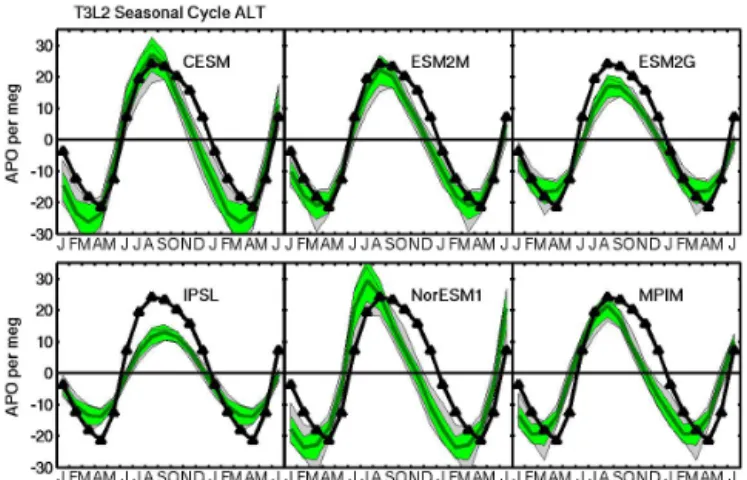
Figure 2e. Results at Alert, Canada (82.5◦N, 62.5◦W), compared to SIO observations.
seasonal maximum was identified. The same approach was used to derive the day of the seasonal NPP maximum, ex-cept that the fit was applied to monthly mean satellite-derived and ESM NPP integrals summed from 40 to 60◦S and 40 to 60◦N, which were compared to the APO phase metric at southern and northern stations, respectively.
3 Results
3.1 APO comparison to ESMs
The APO cycles estimated from the six sets of ESM air– sea fluxes were compared to observations at three South-ern Ocean and two northSouth-ern monitoring sites (Fig. 2). In these plots, the green envelope reflects our best estimate of the ATM uncertainty in the ocean model APO signal based on the nine scaled ATM results, while the gray window re-flects the more complete range of uncertainty using all 13 unscaled ATM results. In general, the distinction between the green and gray windows is only moderately important, as the
observed APO cycle in most cases either falls within both envelopes or lies outside of both envelopes.
The MPIM and related NorESM1 ocean biogeochemistry models are examples in which the observed APO cycle lies outside both ranges of uncertainty at all five evaluation sites (Fig. 2, lower middle and right panels). For these models, the rise in the APO cycle occurs too early in the springtime in both hemispheres, while the overall amplitude of the cycle is too large at all the southern stations. Here, it is notable that the MPIM APO amplitude would be even larger in the South-ern Ocean if it were not offset by the unrealistically large seasonal cycle in oceanic CO2 described above. The large
CO2cycle, however, does not substantially alter the phase of
APO, which is determined mainly by the timing of the O2
fluxes.
The IPSL is another ocean biogeochemistry model for which the observed APO cycle lies outside of both the best guess and full range of uncertainty at all monitoring sites, with the exception of Palmer Station (64.9◦S), where ob-served APO falls within the wider gray window of uncer-tainty (Fig. 2b, lower left panels). Unlike the MPIM and NorESM1, the rise in the IPSL APO cycle occurs somewhat later in the springtime than observed, while the overall am-plitude of the cycle tends to be underestimated. The under-estimate is mild at all the southern stations, and even falls within the broader range of uncertainty at PSA, but is more pronounced at the northern monitoring sites, where the IPSL amplitude is too small by nearly a factor of 2.
The CESM is the top performer among the six ESMs evaluated, consistently yielding green (gray) windows that encompass the observed APO cycle at most (all) of the five monitoring sites (Fig. 2, upper left panels). The GFDL ESM2M (depth-based coordinates) is the second most con-sistent performer, yielding cycles that generally agree with observations, with exceptions at BRW, where ESM2M tends to mildly underestimate the depth of the APO trough, and at PSA, where the rise in the APO cycle may be up to 1 month too early. The sigma-coordinate GFDL ESM2G model is the third best performer, capturing the observed APO cycle rela-tively well at most southern stations, but underestimating the seasonal amplitude at the northern stations.
3.1.1 Regional analysis of APO cycle
The matrix method can partition the ocean model APO cy-cles into regional contributions from the 11 ocean regions used in T3L2. At the southern stations of SPO, PSA and MQA, this partitioning reveals, not surprisingly, that the Southern Ocean (defined as all ocean regions south of 44◦S) dominates the APO cycle (not shown). However, at BRW and ALT at least three regions make important contributions, in-cluding the temperate North Pacific (extending from 15◦N to the Bering Strait around 65◦N and thus including the sub-polar region), the temperate North Atlantic (extending from 15 to 48◦N) and the Northern Ocean (including the Arctic
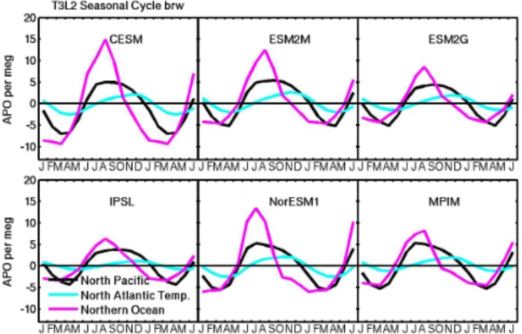
Figure 3. Partitioning the APO cycle at Barrow, Alaska, into its main regional contributions, North Pacific (black), temperate North Atlantic (cyan) and Northern Ocean (magenta), which includes the North Atlantic north of 48◦N and the Arctic Ocean. All curves re-flect the unscaled model mean of the 13 ATMs used in the matrix method.
Ocean and the North Atlantic north of 48◦N). The Northern Ocean is the most important contributor to the APO seasonal cycle at both BRW (Fig. 3) and ALT and is by far the most variable component among the six ESMs. The largest APO amplitudes in the Northern Ocean are produced by the CESM and NorESM1, which are the only two models that capture the total observed APO amplitude at BRW (Fig. 2d).
3.1.2 Partitioning of APO cycle among component signals
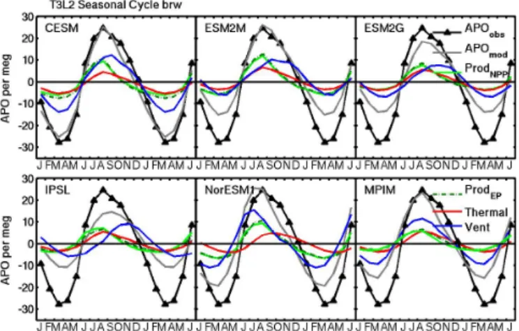
To probe further into the underestimate of the APO amplitude at BRW by most of the ESMs, we partitioned APO into ther-mal and NCP-related components, as described in Sect. 2.2.3 (Fig. 4). A comparison of the CESM and ESM2M in Fig. 4 indicates that both have similar APOthermand APONCP
sig-nals, but that the CESM captures total APO more or less correctly while ESM2M underestimates the total APO am-plitude. By inference, the missing APOventterm accounts for
the difference. However, as discussed in Sect. 2.2.3, APOvent
can be estimated only as a residual of three other terms us-ing standard CMIP5 output and thus its shape and phasus-ing are sensitive to even small uncertainties in those other terms. Thus, the residual ventilation curves in Fig. 4 should be inter-preted with caution (e.g., the MPIM curve is clearly unrea-sonable in phasing). The four remaining ESMs have APONCP
cycles of similar or smaller amplitude than the CESM, which in the case of the ESM2G and MPIM is due primarily to their relatively low export fraction ratios (ef ratios), and all these models substantially underestimate the total APO amplitude at BRW. This suggests that these models probably also un-derestimate some combination of deep ventilation and NCP.
A similar partitioning of APO was attempted in the South-ern Ocean, but the estimation of APONCPfrom model EP100
Figure 4. Partitioning of the model mean APO cycle into NCP, ther-mal and residual ventilation components at Barrow, Alaska. The APONCP components are estimated alternatively based on ocean model EP at 100m (ProdEPlight green, solid curve) and vertically
integrated NPP (ProdNPP)scaled by the mean ratio of EP100/NPP
(f ratio) between 40 and 60◦N of the given ocean model (dark green, dashed curve). All components were translated into atmo-spheric signals as described in Sect. 2.2.3. Also shown is APOvent
(blue), calculated as a residual of APO – APONCP – APOtherm.
With the exception of observed APO, all curves reflect the unscaled mean of the 13 ATMs used in the matrix method.
generally did not give plausible results in this region. This problem is discussed in more detail in Sect. 4.
3.2 Satellite data compared to ESMs
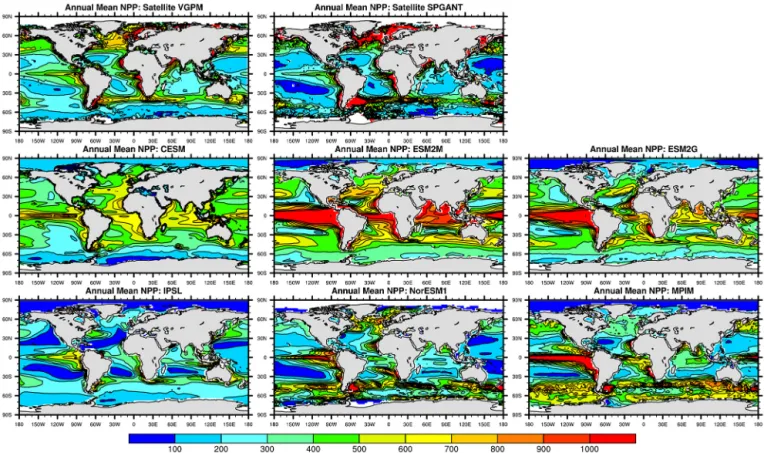
Estimates of NPP display a wide variety of spatial pat-terns among models and satellite data (Fig. 5). Global to-tals range over more than a factor of 2 (34–82 Pg C yr−1) among the ESMs, with most models tending to exceed the VGPM satellite-based estimate of 45 Pg C yr−1 (Table 1). Global EP is more consistent among the models, with a value around 8 Pg C yr−1 in most cases, in good agreement with the satellite-based estimate. Global EP converges among the ESMs because the model with the highest global NPP (ESM2M) has the smallest ef ratio of < 0.1 and the mod-els with the lowest global NPP (IPSL, NorESM1) have the largest ef ratios of about 0.2 (Table 1).
The high global NPP totals in the ESMs are driven in large part by high tropical NPP values, which generally are not re-flected in the satellite data except along coastlines (Fig. 5). In this paper, we focus on the 40–60◦latitude bands, which are more important than the tropics in driving the seasonal cy-cles in NPP, EP (NCP) and APO (Garcia and Keeling, 2001; Anav et al., 2013). In the Southern Ocean 40–60◦S band, global NPP ranges among ESMs from 5.2 to 12.5 Pg C yr−1, encompassing the satellite-based estimates (Table 1, Fig. 6). However, the ESMs tend to underestimate EP relative to the satellite-derived values, particularly the SPGANT Laws (2004) model, due largely to the small model ef ratios. In
the 40–60◦N band, the ESMs generally underestimate both NPP and ef ratios relative to the satellite-derived values. This combination leads to model EP values that are smaller than satellite EP by a factor of 2 on average (Table 1). In both hemispheres, the model NPP maximum tends to occur ear-lier than the satellite-derived maximum, with some mod-els (IPSL, MPIM) predicting a maximum that is up to 1– 2 months early (Fig. 6).
3.3 Combining APO and satellite data
In the previous sections we considered APO and satellite data as separate evaluation metrics for ESMs. Below we consider the two as combined metrics. While this analysis is limited by uncertainties in the absolute magnitude of satellite NPP and EP/NCP and our imperfect ability to partition the ESM total APO signal into its NCP and other components, it nev-ertheless provides some additional insight into the behavior of the ESMs.
3.3.1 Phase metrics
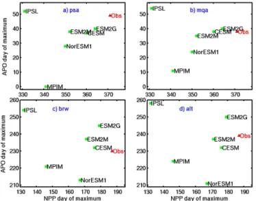
The phase metrics defining the timing of the observed and model seasonal maximum in APO reveal characteristic pat-terns for each ESM, which are relatively consistent across APO monitoring sites (Fig. 7). The APO seasonal maxima of the MPIM and NorESM1 are earlier than observed by about 1 month and 3 weeks, respectively, on average, while the IPSL APO maximum (with the exception of PSA) tends to be later than observed by 2–3 weeks. The remaining models, CESM, ESM2M and ESM2G, have seasonal APO maxima that are relatively consistent with observations, although with some variation among different stations.
The observed seasonal maximum of NPP occurs about 30–40 days earlier than the observed APO maximum in the Southern Ocean stations and about 50 days earlier at BRW and ALT. Of the models, ESM2G, CESM and ESM2M cap-ture the phase of the NPP maximum to within about 1–3 weeks, although as noted above in Fig. 6 the model NPP maxima tend to occur earlier than the satellite-based maxima. In the MPIM, the NPP maximum is about 1 to 1.5 months earlier than observed, and the APO maximum is also cor-responding early (Fig. 7). The IPSL is an outlier from the general slope of the APO vs. NPP phase relationship, as de-fined by the rest of the ESMs. The IPSL NPP maximum occurs about 40 days earlier than observed in the South-ern Hemisphere and nearly 2 months earlier than observed in the Northern Hemisphere, but the IPSL, curiously, also has the latest APO seasonal maximum of any of the mod-els. NorESM1 is another outlier in the opposite direction off the general APO vs. NPP phase slope, at least in the North-ern Hemisphere. There, NorESM1’s seasonal maximum in NPP has a relatively small lag from the APO maximum com-pared to the other models. NorESM1 is also unusual in that
Figure 5. Annual mean NPP (in mg C m−2day−1). Top row: MODIS-Aqua data input to the VGPM NPP model and (b) SeaWiFS data input to the SPGANT algorithm as described in Nevison et al. (2012a). Rows 2 and 3 show the corresponding NPP fields from six ESMs for the mean of 1997–2005.
Figure 6. Comparison of the NPP (PgC month) mean annual cy-cle as simulated by ESMs and satellite-derived observations inte-grated over (a) 40–60◦S, (b) 40–60◦N, (c) 60–90◦N. The satellite data are from SPGANT Laws (2004) model in panel (a) and VGPM Dunne model in panels (b–c).
the APOtherm seasonal maximum at Barrow occurs about 1
month later than in any of the other ESMs (Fig. 4).
3.3.2 Seasonal amplitudes
In addition to evaluating the phasing of the ocean model APO and NPP cycles, we examined the amplitude of the cycles, with the caveat that the absolute magnitude of satellite-based NPP is not well determined and at present provides a rela-tively weak constraint on the models. Furthermore, the APO seasonal amplitude in principle is more closely related to NCP (or EP) than NPP. However, we chose NPP for the sea-sonal amplitude analysis due to the strong discrepancies in ef ratio among models and satellite data indicated in Table 1, which may unduly bias the results.
A cross plot of the seasonal amplitude in APO against the seasonal amplitude of NPP integrated between 40 and 60◦S suggests a strong correlation between the amplitudes of APO and NPP among the ocean biogeochemistry mod-els, with larger NPP amplitudes associated with larger APO cycles. The strong correlation holds at all Southern Ocean stations and is illustrated in Fig. 8a at MQA. The cluster of top-performing ESMs (CESM, ESM2M, ESM2G) agrees relatively well with the observed APO and SPGANT ampli-tudes. Meanwhile both amplitudes are underestimated by the IPSL and overestimated by the NorESM1 and MPIM.
Cross plots of the seasonal amplitudes of APO and NPP in the Northern Hemisphere reveal that these amplitudes
Figure 7. Day of APO maximum plotted against day of NPP maximum. The observed data point is derived from APO data at (a) Palmer Station, (b) Macquarie Island, (c) Barrow and (d) Alert plotted against satellite NPP data integrated over the 40–60◦ lati-tude band of the appropriate hemisphere.
are positively correlated at BRW (Fig. 8b) and ALT (not shown), although the correlation is weaker than in the South-ern Hemisphere. The CESM, ESM2G, ESM2M and MPIM all capture the satellite-based NPP seasonal amplitude rela-tively well, while both the CESM and NorESM1 capture the observed APO amplitude accurately. However, the CESM is the only model that reproduces both the NPP and APO sea-sonal amplitudes well relative to the observations.
4 Discussion 4.1 Northern oceans
Most ESMs tend to underestimate substantially the observed seasonal amplitude of APO at Barrow, Alaska. A combina-tion of region-specific results (Fig. 3) and O2 component
analysis (Fig. 4) suggests that some combination of fall– winter deep ventilation and spring–summer EP in the north-ern oceans (defined to include the North Atlantic north of 48◦N) in particular may be underestimated in many models. The combined analysis of the APO vs. NPP seasonal am-plitudes (Fig. 8b) supports these conclusions and suggests that, while several models may be capturing primary pro-duction well in the northern oceans, accurate representation of EP and deep ventilation is also important for reproducing the observed APO cycle. The inference from the APO com-ponent analysis in Fig. 4 that the GFDL models may have weak ventilation in the North Atlantic appears to contradict the analysis of Dunne et al. (2012), who found robust North Atlantic Deep Water (NADW) formation in both the ESM2M and ESM2G versions, but possibly could be reconciled if the
Figure 8. (a) Seasonal amplitude in APO at Macquarie Island (MQA), located at 54.5◦S, 159◦E, as estimated from the air–sea O2, CO2and heat fluxes from six ESMs, plotted against the sea-sonal amplitude of NPP integrated from 40 to 60◦S. Error bars rep-resent the ATM uncertainty in model APO as estimated with the matrix method. The observed (Obs) data points (in red) are based on APO data from the PU network at MQA and NPP from the SP-GANT satellite ocean color algorithms, as described in the text. The correlation coefficient R refers to regression through ESM points only, (b) Same as 8a, but plotting seasonal amplitude in APO at Barrow, Alaska, against the seasonal amplitude of NPP integrated from 40 to 60◦N. The observed data point is based on APO data from the PU network and the VGPM algorithm with MODIS-Aqua input.
biogeochemical gradients across which deep water formation acts are too weak.
We investigated several mechanisms that might explain the differences among models in the APO cycle at high northern latitudes, including subpolar heat transport and Arctic sea ice cover. Here, stronger northward heat transport should lead to more deep ventilation, while lower sea ice cover will permit more production and ventilation in the Arctic Ocean. Sub-dividing the northern oceans region into the Arctic Ocean and North Atlantic components revealed that some models (IPSL and ESM2G) have a very small component (< 2 per meg) of APO seasonal amplitude coming from the Arctic Ocean alone (Fig. 9). In ESM2G this may be related to the extensive winter sea ice cover, which exceeds the observed covered area reported by the National Snow and Ice Data Center (http://nsidc.org/data/seaice_index/archives.html) by about 2 × 10⁶km2. However, sea ice cover is lower than observed in the IPSL, suggesting the small Arctic APO
Figure 9. APO cycle at Barrow, Alaska, from the TransCom north-ern oceans region, restricted to latitudes north of 65◦N to estimate the contribution of the Arctic Ocean. All curves reflect the unscaled model mean of 13 ATMs used in the matrix method.
component in that model is more related to general underes-timate of primary and EP (e.g., as shown in Figs. 6b and 8b). While it seems clear that the strong APO seasonality in the CESM can be attributed in part to its high productivity and EP in the northern subpolar and polar regions (Fig. 6 and Ta-ble 1), a full explanation for the underlying mechanisms of the CESM fidelity on APO compared to the other models is not readily apparent from surface-only data. This suggests the need for a more detailed exploration of ocean interior ventilation and biological response interactions outside the scope of the present work.
4.2 Southern Ocean
Compared to the Northern Hemisphere stations, the ESMs generally are more successful in the Southern Ocean in cap-turing the observed APO cycle (Fig. 2). Within the range of ATM uncertainty, at least three models, CESM, ESM2M, ESM2G (and IPSL at Palmer Station), predict seasonal APO amplitudes in agreement with observations. Although the Southern Ocean APO amplitude in these models varies over as much as 20 per meg, we currently are not able to distin-guish which of the underlying air–sea O2 flux fields is the
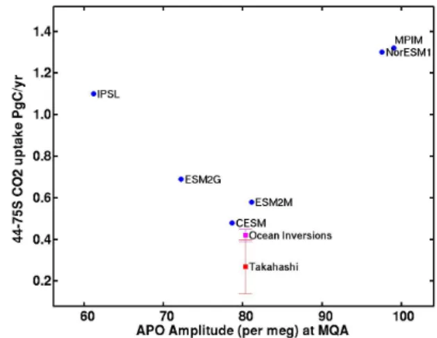
most realistic, due to the uncertainty associated with translat-ing these fluxes into an atmospheric signal ustranslat-ing TransCom3 era model responses to uniformly distributed regional fluxes. However, even with our current matrix method, the APO con-straint is sufficiently robust to indicate that the NorESM1 and MPIM substantially overestimate some combination of pro-duction and deep ventilation in the Southern Ocean, while the IPSL probably tends to underestimate these fluxes (Ta-ble 1, Fig. 8a). Notably, the ESMs that reproduce APO the best in the Southern Ocean tend to predict a smaller net car-bon uptake between 44 and 75◦, and are in better agreement with independent estimates (Lenton et al., 2013) of carbon
Figure 10. Annual mean CO2 uptake in the Southern Ocean for
1997–2005 integrated from 44–75◦S and plotted vs. mean APO amplitude at Macquarie Island (MQA) over the same period, as predicted by six ESMs. Independent estimates of carbon uptake from ocean inversions and observed pCO2databases (Lenton et al.,
2013), plotted against the observed APO amplitude at MQA are shown for reference.
uptake from ocean inversions and observed pCO2databases
(Fig. 10).
Reducing ATM uncertainty is a challenge that potentially can be addressed by using column-integrated APO signals from aircraft data (Wofsy, 2011), or conversely, by using vertical profiles to identify top-performing ATMs (Stephens et al., 2007). In addition, the spread in ATM results has been reduced substantially for CO2 inversions using
post-TransCom3-era ATMs (Peylin et al., 2013), suggesting that ATM uncertainty also may be reduced for forward tions of APO. If this is the case, then new forward simula-tions with several different modern-era ATMs may be suffi-cient to characterize ATM uncertainty. Alternatively, it may be valuable to continue with a matrix-based approach, us-ing basis functions from many ATMs, but with redefined re-gional boundaries that are not defined based simply on lat-itude, as in T3L2 (Fig. 1), but rather that correspond to the biogeography of major ocean regions (Fay and McKinley, 2014). The definition of such basis functions could help ex-tend the utility of the matrix approach to lower latitude APO monitoring sites and allow for the partitioning of the South-ern Ocean into multiple regions defined around biogeochem-ical function, while still retaining the advantages of the ma-trix method, i.e., the ability to quickly and easily compare multiple ATMs forced with the same air–sea fluxes.
A second complication in the Southern Ocean analysis is that the EP100values reported by the ESMs clearly are not
di-rectly comparable to satellite NCP(EP) data, particularly our SPGANT product, and thus can not be translated with confi-dence into air–sea O2fluxes associated with NCP. A likely
problem is that the 100 m depth horizon used to compute EP may not be comparable across satellite algorithms and
ocean biogeochemistry models. EP100will underestimate the
model’s true NCP-related O2outgassing flux if organic
mat-ter is respired as it sinks from the actual model mixed layer depth to 100 m depth (Najjar et al., 2007). It is also puzzling that the ef ratios predicted by the ESMs (Table 1) appear to have decreased considerably in some cases relative to those reported for earlier versions of the same models (Steinacher et al., 2010). For example, the Southern Ocean ef ratios for the MPIM and IPSL in that earlier study were about 0.2 and 0.4, respectively, compared to 0.14 and 0.27, respectively, in the current study. The mean global ef ratio for the six ESMs in the current study is only 0.14 and, even in the Southern Ocean, is only 0.17 on average, compared to satellite-based estimates of 0.18 globally and about 0.3 at high latitudes.
The small ef ratios in the GFDL models (of less than 0.1 globally and only 0.10 to 0.13 in the Southern Ocean) ap-pear consistent with the relatively deep summer mixed layer depths (MLDs) in the Southern Ocean, which even at their minimum are often deeper than 100 m in both ESM2M and ESM2G (Dunne et al., 2012). In the CESM the Southern Ocean summer MLDs are generally shallower than 100 m and in many regions are only around 10–40 m deep (Moore et al., 2013). The shallower summer MLDs may contribute to the CESM’s larger ef ratio of 0.18, although this ratio is still small compared to the satellite-based estimates. The small GFDL ef ratios may also be related to an overvigorous pi-cophytoplankton component wherein a prochlorococcus-like form is capable of competing relatively well even in cold po-lar waters. Small picophytoplankton are more likely to be re-oxidized and remineralized within the mixed layer, whereas larger, heavier microphytoplankton (e.g., diatoms) are more likely to be exported out of the oceanic mixed layer (Uitz et al., 2010).
4.3 Phase relationships
While much of our analysis focuses on the seasonal am-plitude of APO and NPP at mid- to high latitudes, both of these metrics involve relatively large uncertainty. This de-rives from TransCom3-era uniform flux ATM uncertainty in the case of APO, while for NPP the uncertainty results from the lack of strong constraints on the absolute magnitude of the satellite fluxes. In contrast, we have relatively high con-fidence in the phasing of model APO, as represented by the matrix method (see the Supplement) and in NPP observa-tionally derived from satellite data, based on the close corre-spondence in phasing between the SPGANT and VGPM al-gorithms. For these reasons, we used a phase metric, i.e., the timing of the seasonal maximum, to examine relationships between observed and model APO and NPP. As in the sea-sonal amplitude analysis, MPIM, NorESM1 and IPSL dis-played phasing patterns that tended to deviate from obser-vations and the other three top-performing models, albeit in diverging ways. A complete diagnosis of the model physics responsible for the phasing anomalies (e.g., IPSL’s early NPP
maxima and late APO maxima) described in Sect. 3.3.1 is beyond the scope of this paper. Here we note mainly that the phase metrics are a robust and relatively good indicator of overall model performance with respect to APO.
5 Summary
We have used measurements of the seasonal cycles in APO to challenge and test the ocean model components of six ESMs. The model/data comparison reveal that three of the ESMs tested reproduce the observed cycles reasonably well, within the range of ATM uncertainty, while three do not. ESM per-formance in general is more favorable in the Southern Hemi-sphere than in the Northern HemiHemi-sphere, where most mod-els appear to underestimate the wintertime ventilation of O2-depleted deepwater that drives the declining branch of
the APO seasonal cycle and many may also underestimate both primary and EP, particularly at high northern latitudes. We used NPP and NCP(EP) products derived from satellite ocean color data as complementary constraints on the mod-els in an effort to tighten the APO constraint, which reflects a combination of production and ventilation processes. How-ever, while the satellite data provide relatively strong con-straints with respect to phasing, they are more uncertain with respect to the absolute magnitudes of NPP and NCP(EP).
At least two primary uncertainties limit our ability to place stronger constraints on ocean model biogeochemistry based on currently available information from APO and satellite data: (1) the relatively large ATM uncertainty involved in translating air–sea O2fluxes into APO signals. (2) The
uncer-tainty in how model EP100relates to the true model FO2,NCP
flux and how this relationship varies across models and satel-lite algorithms. The first of these, ATM uncertainty, is large, as quantified using our TransCom3-based matrix method. However, it probably has been overstated in previous anal-yses, which in some cases went so far as to suggest that APO does not provide a useful constraint on ocean model fluxes (e.g., Naegler et al., 2007). Further, ATM uncertainty could be reduced substantially in future work with modern ATMs and O2-specific flux patterns, or with new regional
bound-aries defined based on ocean biogeography rather than sim-ple latitude. Even within the limits of our current approach, we have shown that half of the six ESMs tested here produce APO cycles whose mismatch with observed APO clearly transcends ATM uncertainty, suggesting underlying deficien-cies in those models’ physics and biogeochemistry.
Improving the understanding of the relationship between model air–sea O2fluxes and quantities like NPP, NCP and EP
is a more tractable problem that can be dissected with appro-priate model diagnostics, e.g., as per Manizza et al. (2012). In the current analysis, using standard CMIP5 output from six ocean biogeochemistry models, we encountered difficulties in relating FO2to EP and NCP, which hindered our ability to
and to compare ESM-derived APONCP directly to
satellite-based APONCPsignals. Extending model-derived insights to
satellite products likely will require a shift in emphasis from EP at an arbitrary reference depth to near-surface processes like NCP, which are more relevant for exchanges of O2and
CO2at the air–sea interface and more directly related to
up-ward radiances detected by satellites.
The Supplement related to this article is available online at doi:10.5194/bg-12-193-2015-supplement.
Acknowledgements. The authors gratefully acknowledge the
CMIP5 ocean modelers for providing the output that made this project possible. In particular, we thank Keith Lindsay, Laure Resplandy and Cristoph Heinze for their assistance. We also thank Britt Stephens and an anonymous reviewer for their helpful comments, which much improved the manuscript. Lastly, we thank Michael Bender and Robert Mika for providing APO data and acknowledge support from NASA Ocean Biology and Biogeochemistry grant NNX11AL73G.
Edited by: M. Heimann
References
Anav, A., Friedlingstein, P., Kidston, M., Bopp, L., Ciais, P., Cox, P., Jones, C., Jung, M., Myneni, R., and Zhu, Z. : Evaluating the Land and Ocean Components of the Global Carbon Cycle in the CMIP5 Earth System Models, J. Climate, 26, 6801–6843, 2013. Arora, V. K., Boer, G. J., Friedlingstein, P., Eby, M., Jones, C., Christian, J., Bonan, G., Bopp, L., Brovkin, V., Cadule, P., Ha-jima, T., Ilyina, T. Lindsay, K, Tjiptura, J., and Wu, T.: : Carbon– Concentration and Carbon–Climate Feedbacks in CMIP5 Earth System Models. J. Climate, 26, 5289–5314, 2013.
Aumont, O. and L. Bopp: Globalizing results from ocean in situ iron fertilization studies, Glob. Biogeochem. Cy., 20, GB2017, doi:10.1029/2005GB002591, 2006.
Battle, M., Mikaloff Fletcher, S., Bender, M. L., Keeling, R. F., Manning, A. C., Gruber, N., Tans, P. P., Hendricks, M. B., Ho, D. T., Simonds, C., Mika, R., and Paplawsky, B.: Atmospheric potential oxygen: New observations and their implications for some atmospheric and oceanic models, Glob. Biogeochem. Cy., 20, GB1010, doi:10.1029/2005GB002534, 2006.
Behrenfeld, M. J. and Falkowski, P. G.: Photosynthetic rates de-rived from satellite based chlorophyll concentration, Limnol. Oceanogr., 42, 1–20, 1997.
Bender, M., Ellis, J. T., Tans, P. P., Francey, R. J., and Lowe, D.: Variability in the O2/N2ratio of southern hemisphere air, 1991–
1994: implications for the carbon cycle, Global Biogeochem. Cy., 10, 9–21, 1996.
Bender, M., Ho, D., Hendricks, M. B., Mika, R., Battle, M. O., Tans, P., Conway, T. J., Sturtevant, P. B., and Cassar, N.: Atmospheric O2/N2changes, 1993-02002: Implications for the partitioning
of fossil fuel CO2 sequestration, Global Biogeochem. Cy., 19, GB4017, doi:10.1029/2004GB002410, 2005.
Blaine, T. W.: Continuous Measurements of Atmospheric Ar/N2as a Tracer of Air-Sea Heat Flux: Models, Methods, and Data, Uni-versity of California, San Diego, La Jolla, 22–66, 2005. Bopp, L., Resplandy, L., Orr, J. C., Doney, S. C., Dunne, J. P.,
Gehlen, M., Halloran, P., Heinze, C., Ilyina, T., Séférian, R., Tjiputra, J., and Vichi, M.: Multiple stressors of ocean ecosys-tems in the 21st century: projections with CMIP5 models, Biogeosciences, 10, 6225–6245, doi:10.5194/bg-10-6225-2013, 2013.
Boyd, P. W. and Doney, S. C.: The impact of Climate Change and Feedback Processes on the Ocean Carbon Cycle, Chapter 7 ,in: The role of the Ocean Carbon Cycle in Global Change, edited by: Fasham, M. J. R., Ocean Biogeochemistry, Springer-Verlag, 157–198, 2003.
Dunne, J. P., Armstrong, R. A., Gnanadesikan, A., and Sarmiento J. L.: Empirical and mechanistic models for the parti-cle export ratio, Global Biogeochem. Cy., 19, GB4026, doi:10.1029/2004GB002390, 2005.
Dunne, J. P., John, J., Adcroft, A., Griffies, S., Hallberg, R., Shevli-akova, E., Stouffer, R., Cooke, W., Dunne, K., Harrison, M., Krasting, J., Malyshev, S., Milly, P., Phillips, P., Sentman, L., Samuels, B., Spelman, M., Winton, M., Wittenberg, A., and Zadeh, N.: : GFDL’s ESM2 global coupled climate-carbon Earth System Models Part I: Physical formulation and baseline simula-tion characteristics, J. Clim., 25, 6646–6665, doi:10.1175/JCLI-D-11-00560.1, 2012
Dunne, J. P., John, J., Shevliakova, E., Stouffer, R., Krasting, J., Malyshev, S., Milly, P., Sentman, L., Adcroft, A., Cooke, W., Dunne, K., Griffies, S., Hallberg, R., Harrison, M., Levy, H., Wit-tenberg, A., Phillips, P., and Zadeh, N.: GFDL’s ESM2 global coupled climate-carbon Earth System Models Part II: Carbon system formulation and baseline simulation characteristics, J. Clim., 26, 2247–2267, doi:10.1175/JCLI-D-12-00150.1, 2013. Fay, A. R. and McKinley, G. A.: Global open-ocean biomes: mean
and temporal variability, Earth Syst. Sci. Data, 6, 273–284, doi:10.5194/essd-6-273-2014, 2014.
Garcia, H. E. and Keeling, R. F.: On the global oxygen anomaly and air-sea flux, J. Geophys. Res., 106, 31155–31166, 2001. Gruber, N. and Sarmiento, J. L.: Large-scale
biogeochemical-physical interactions in elemental cycles, in: The Sea, Volume 12, edited by: Robinson, A. R., McCarthy, J. J., and Rothschild, B. J., John Wiley & Sons, Inc., New York, 337–399, 2002. Gurney, K. R., Law, R., Denning, A. S., Rayner, P., Baker, D.,
Bousquet, P., Bruhwiler, L., Chen, Y.-H., Ciais, P., Fan, S., Fung, I., Gloor, M., Heimann, M., Higuchi, K., John, J., Kowal-czyk, E., Maki, T., Maksyutov, S., Peylin, P., Prather, M., Pak, B., Sarmiento, J., Taguchi, S., Takahashi, T., and Yuen, C.-W.: Transcom 3 CO2 inversion intercomparison: 1. Annual mean
control results and sensitivity to transport and prior flux infor-mation, Tellus, 55, 555–579, 2003.
Gurney, K. R., Law, R., Denning, A. S., Rayner, P., Pak, B., Baker, D., Bousquet, P., Bruhwiler, L., Chen, Y.-H., Ciais, P., Fan, S., Fung, I., Heimann, M., John, J., Maki, T., Maksyutov, S., Peylin, P., Prather, M., and Taguchi, S.: Transcom 3 inversion intercom-parison: Model mean results for the estimation of seasonal car-bon sources and sinks, Global Biogeochem. Cy., 18, GB1010, doi:10.1029/2003GB002111, 2004.
Henson, S., Cole, H., Beaulieu, C., and Yool, A.: The impact of global warming on seasonality of ocean primary production,
Biogeosciences, 10, 4357–4369, doi:10.5194/bg-10-4357-2013, 2013.
Ilyina, T., Six, K. D., Segschneider, J., Maier-Reimer, E., Li, H., and Nuñez-Riboni, I.: Global ocean biogeochemistry model HAMOCC: Model architecture and performance as component of the MPI-Earth system model in different CMIP5 experi-mental realizations, J. Adv. Model. Earth Syst., 5, 287–315, doi:10.1029/2012MS000178, 2013.
Jin, X., Najjar, R. G., Louanchi, F., and Doney, S. C.: A modeling study of the seasonal oxygen budget of the global ocean, J. Geo-phys. Res., 112, C05017, doi:10.1029/2006JC003731, 2007. Kahru, M. and Mitchell, B. G.: Blending of ocean colour algorithms
applied to the Southern Ocean, Remote Sens. Lett., 1, 119–124, doi:10.1080/01431160903547940, 2010.
Kahru, M., Kudela, R., Manzano-Sarabia M., and Mitchell, B. G.: Trends in primary production in the California Current detected with satellite data, J. Geophys. Res., 114, C02004, doi:10.1029/2008JC004979, 2009.
Keeling, R. F., Najjar, R. P., Bender, M. L., and Tans, P. P.: What atmospheric oxygen measurements can tell us about the global carbon cycle, Global Biogeochem. Cy., 7, 37–67, 1993. Keeling, R. F., Stephens, B. B., Najjar, R. G., Doney, S. C., Archer,
D., and Heimann, M.: Seasonal variations in the atmospheric O2/N2ration in relation to the kinetics of air-sea gas exchange,
Global Biogeochem. Cy., 12, 141–163, 1998.
Keeling, R. F., Koertzinger, A., and Gruber, N.: Ocean Deoxygena-tion in warming world, Annu. Mar. Rev. Sci., 2, 463–493, 2010. Khatiwala, S., Primeau, F., and Hall, T.: Reconstruction of the his-tory of anthropogenic CO2concentrations in the ocean, Nature,
462, 346–350, 2009.
Laws, E. A.: Export flux and stability as regulators of community composition in pelagic marine biological communities: Implica-tions for regime shifts, Progr. Oceanogr., 60, 343–353, 2004. Laws, E. A., Falkowski, P. G., Smith, W. O., Jr., Ducklow, H. W.,
and McCarthy, J. J.: Temperature effects on export production in the open ocean, Global Biogeochem. Cy., 14 1231–1246, 2000. Lee, Z., Lance, V., Shang, S., Vaillancourt, R., Freeman, S.,
Lubac, B., Hargreaves, B., Del Castillo, C., Miller, R., Twar-dowski, M., and Wei, G.: : An assessment of optical proper-ties and primary production derived from remote sensing in the Southern Ocean (SO GasEx), J. Geophys. Res., 116, C00F03, doi:10.1029/2010JC006747, 2011.
Lenton, A., Tilbrook, B., Law, R. M., Bakker, D., Doney, S. C., Gruber, N., Ishii, M., Hoppema, M., Lovenduski, N. S., Matear, R. J., McNeil, B. I., Metzl, N., Mikaloff Fletcher, S. E., Monteiro, P. M. S., Rödenbeck, C., Sweeney, C., and Takahashi, T.: Sea-air CO2fluxes in the Southern Ocean for the period 1990–2009,
Biogeosciences, 10, 4037–4054, doi:10.5194/bg-10-4037-2013, 2013.
Le Quéré, C., Roedenbeck, C., Buitenhuis, E. T., Conway, T. J., Langenfelds R., Gomez, A., Labuschagne, C., Ramonet, M., Nakazawa, T., Metzl, N., Gillett, N., and Heimann, M: Saturation of the Southern Ocean CO2sink due to recent climate change,
Science, 316, 1735–1738, 2007.
Manizza, M., Keeling, R. F., and Nevison, C. D.: On the pro-cesses controlling the seasonal cycles of the air-sea fluxes of O2 and N2O: A modeling study, Tellus B, 64, 18429,
doi:10.3402/tellusb.v64i0.18429, 2012.
Manning, A. C. and Keeling, R. F.: Global oceanic and land biotic carbon sinks from the Scripps atmospheric oxygen flask sam-pling network, Tellus B, 58B, 95–116, 2006.
Mitchell, B. G.: Predictive bio-optical relationships for polar oceans and marginal ice zones, J. Mar. Sys., 3, 91–105, 1992.
Mitchell, B. G. and Kahru, M.: Bio-optical algorithms for ADEOS-2 GLI, J. Remote Sens. Soc., ADEOS-29, 1, 80–85, ADEOS-2009.
Moore, J. K., Doney, S. C., Kleypas, J. C., Glover, D. M., and Fung, I. Y.: An intermediate complexity marine ecosystem model for the global domain, Deep-Sea Res.-Pt. II, 49, 403–462, 2002. Moore, J. K., Doney, S. C., and Lindsay, K.: Upper ocean ecosystem
dynamics and iron cycling in a global 3-D model, Global Bio-geochem. Cy., 18, GB4028, doi:10.1029/2004GB002220, 2004. Moore, J., Lindsay, K., Doney, S., Long, M., and Misumi, K.: Ma-rine Ecosystem Dynamics and Biogeochemical Cycling in the Community Earth System Model [CESM1(BGC)]: Comparison of the 1990s with the 2090s under the RCP4.5 and RCP8.5 Scenarios, J. Climate, 26, 9291–9312, doi:10.1175/JCLI-D-12-00566.1, 2013.
Naegler, T., Ciais, P., Orr, J., Aumont, O., and Roedenbeck, C.: On evaluating ocean models with atmospheric potential oxygen, Tel-lus, 59B, 138–156, 2007.
Najjar, R. G.,Jin, X, Louanchi, F., Aumont, O., Caldeira, K., Doney, S., Dutay, J. C., Follows, M., Gruber, N., Joos, F., Lindsay, K., Maier-Reimer, E., Matear, R., Matsumoto, K., Monfray, P., Mouchet, A., Orr, J., Plattner, G. K., Sarmiento, J., Schlitzer, R., Slater, R., Weirig, M.-F., Yamanaka, Y., and Yool, A: Impact of circulation on export production, dissolved organic matter, and dissolved oxygen in the ocean: Results from Phase II of the Ocean Carbon-cycle Model Intercompari-son Project (OCMIP-2), Global Biogeochem. Cy., 21, GB3007, doi:10.1029/2006GB002857, 2007.
Nevison, C. D., Mahowald, N. M., Doney, S. C., Lima, I. D., and Cassar, N.: Impact of variable air-sea O2and CO2fluxes on
at-mospheric potential oxygen (APO) and land-ocean carbon sink partitioning, Biogeosciences, 5, 875–889, doi:10.5194/bg-5-875-2008, 2008.
Nevison, C. D., Keeling, R. F., Kahru, M., Manizza, M., Mitchell, B. G., and Cassar, N.: Estimating net community production in the Southern Ocean based on atmospheric potential oxygen and satellite ocean color data, Global Biogeochem. Cy., 26, GB1020, doi:10.1029/2011GB004040, 2012a.
Nevison, C. D., Baker, D. F., and Gurney, K. R.: A methodol-ogy for estimating seasonal cycles of atmospheric CO2resulting from terrestrial net ecosystem exchange (NEE) fluxes using the Transcom T3L2 pulse-response functions, Geosci. Model Dev. Discuss., 5, 2789–2809, doi:10.5194/gmdd-5-2789-2012, 2012b. Peylin, P., Law, R. M., Gurney, K. R., Chevallier, F., Jacobson, A. R., Maki, T., Niwa, Y., Patra, P. K., Peters, W., Rayner, P. J., Rödenbeck, C., van der Laan-Luijkx, I. T., and Zhang, X.: Global atmospheric carbon budget: results from an ensemble of atmospheric CO2 inversions, Biogeosciences, 10, 6699–6720,
doi:10.5194/bg-10-6699-2013, 2013.
Sauer, M. J., Roesler, C. S., Werdell, J. P., and Barnard, A.: Under the hood of satellite empirical chlorophyll algorithms: revealing the dependencies of maximum band ratio algorithms on inherent optical properties, Optics Express, 20, 20920–20933, 2012. Schneider, B., Bopp, L., Gehlen, M., Segschneider, J., Frölicher,