Decay dynamics in the coupled-dipole model

HAL Id: hal-01518481

https://hal.archives-ouvertes.fr/hal-01518481

Submitted on 4 May 2017

HAL is a multi-disciplinary open access

archive for the deposit and dissemination of

sci-entific research documents, whether they are

pub-lished or not. The documents may come from

teaching and research institutions in France or

abroad, or from public or private research centers.

L’archive ouverte pluridisciplinaire HAL, est

destinée au dépôt et à la diffusion de documents

scientifiques de niveau recherche, publiés ou non,

émanant des établissements d’enseignement et de

recherche français ou étrangers, des laboratoires

publics ou privés.

M Araújo, William Guerin, Robin Kaiser

To cite this version:

M Araújo, William Guerin, Robin Kaiser. Decay dynamics in the coupled-dipole model. Journal of

Modern Optics, Taylor & Francis, 2018, 65, pp.1345. �10.1080/09500340.2017.1380856�. �hal-01518481�

M. O. Ara´ujo,1, 2 William Guerin,1, ∗ and Robin Kaiser1 1

Universit´e Cˆote d’Azur, CNRS, INPHYNI, France

2

CAPES Foundation, Ministry of Education of Brazil, Bras´ılia, DF 70040-020, Brazil Cooperative scattering in cold atoms has gained renewed interest, in particular in the context of single-photon superradiance, with the recent experimental observation of super- and subradiance in dilute atomic clouds. Numerical simulations to support experimental signatures of cooperative scattering are often limited by the number of dipoles which can be treated, well below the number of atoms in the experiments. In this paper, we provide systematic numerical studies aimed at matching the regime of dilute atomic clouds. We use a scalar coupled-dipole model in the low excitation limit and an exclusion volume to avoid density-related effects. Scaling laws for super- and subradiance are obtained and the limits of numerical studies are pointed out. We also illustrate the cooperative nature of light scattering by considering an incident laser field, where half of the beam has a π phase shift. The enhanced subradiance obtained under such condition provides an additional signature of the role of coherence in the detected signal.

I. INTRODUCTION

Since the seminal work by Dicke in 1954 [1], a vast range of phenomena has been studied in the context of light emission and scattering by an ensemble of N two-level systems [2–10]. More recently, the properties of such situations when only one excitation at most is present in the system has been studied, both theoretically and experimentally (“single-photon superradiance” [11–13]). Some of the theoretical work is based on the study of an effective Hamiltonian, investigating either the escape rates of photons from the system [14], related to the imag-inary part of the effective Hamiltonian, or the eigenval-ues of the complete effective Hamiltonian [15–17], with in particular the prediction of a localization transition in the scalar model, absent in a more complete vectorial model [18–20].

Experimental studies of cooperative effects in atom-light interaction however typically involves an incident laser beam, either driving the system to a steady state, or realizing a pulsed excitation to study the dynamics of collective effects. The experimental signatures studied so far include the momentum transfer to the center of mass of the atomic cloud [21–24] or the light scattered either in the backward direction [25], the forward direction [26– 28], or at different angles [29–31].

Theoretical investigations of interference effects in mul-tiple scattering around the backward direction (coher-ent backscattering) can be performed using an approxi-mate diagrammatic approach [32]. For forward scatter-ing, steady-state properties as well as the dynamics after the switch off of the driving field can be well understood by using a description based on the average refractive in-dex of the cloud [26, 28, 33], as long as the atomic sample remains at low density [27, 34]. However, these efficient theoretical approaches do not allow describing scattering at a random angle, as used in [29–31]. Nevertheless, in

∗_{william.guerin@inphyni.cnrs.fr}

the single scattering limit, an alternative approach has been proposed that allows for analytical predictions of the scattering off axis [35].

One more universal approach to light scattering in any direction, in both single and multiple scattering limits, is the so-called coupled-dipole model [36, 37]. This ap-proach, which can be derived in the low-excitation limit either in a quantum framework or from classical scatter-ing, requires a numerical solution of N coupled equations. The near-field dipole-dipole coupling as well as the polar-ization of the electromagnetic radiation can be taken care of, but a simplified model consists in a scalar description

of the dipole-dipole interaction. Even though not

ex-act, this scalar approximation has the merit of having allowed identifying the important role of near-field cou-pling in the problem of Anderson localization [18, 19], not discussed in the context of single parameter scaling [38]. Another advantage of the scalar model is that it allows the simulation of large optical depth without density-related effects. Indeed, as one typically can use up to

N = 104 atoms in the numerical simulations and the

on-resonance optical depth scales as b0 ∝ N /(k0R)2, the

simulation of b0 ≈20 corresponds to a size of the cloud

of k0R ≈ 20, where k0 =2π/λ is the wavenumber

corre-sponding to the atomic transition and R the size of the atomic cloud. For a fixed number of atoms, larger values

of b0 are thus simulated by smaller values of k0R. This

comes along with larger spatial densities ρ and smaller

interatomic distances d ∼ 1/ρ1/3, yielding for the above

choice of parameters values of k0d ∼ 1. For such

densi-ties, the near-field term of the vectorial coupled-dipole model significantly affects the results. The simulation of the dilute limit realized in the experiments is thus diffi-cult. A good compromise is thus to use the scalar model, keeping in mind that this model features a phase

transi-tion when the density reaches values of ρλ3

≈20 [18, 19].

However, even below this critical density, where one ex-pect the long-range coupling to dominate over the lo-cal coupling, we have noticed that for a randomly-filled cloud of particles, occasionally two atoms will be located at very short distance and pair physics can become

vis-ible [16, 19, 39]. As such pair physics is less probable in the dilute atomic cloud, we have added an exclusion volume around each atom to avoid close distances and related effects. A precise simulation of scaling laws as expected in the large atom number limit is therefore del-icate and the scope of this paper is to provide the sys-tematic studies we have performed to explore super- and subradiance in dilute clouds of cold atoms. We note that the experiments [30, 31] are performed with rubidium atoms, having a degenerate ground state with multiple Zeeman sublevels. The additional complexity related to this degeneracy is largely out of reach for present theo-ries, even though some attempts to take care of effects related to this more complex internal structure of the atoms have been made recently [34, 40].

As a further study of cooperativity, we illustrate the role of coherence in subradiance by applying a recently proposed idea [41] to a realistic experimental geometry. Using a properly phased excitation, we show that the time-dependent scattering is indeed sensitive to the phase profile of the laser field and, more importantly for experi-mental aspects, that such a phased excitation can induce an increase of the subradiant fraction of light by almost one order of magnitude. Controlling the addressed states of the full Hilbert space by engineered steering is a splen-did illustration of the potential of cooperative scattering in such open (quantum) systems.

This paper is organized as follows: in section II, we review the scalar coupled-dipole model we use to de-scribe the interaction between an atomic cloud and a laser beam. In section III, we discuss in more detail the impact of the exclusion condition to avoid close atomic pairs and we present scaling laws of super- and subra-diance obtained in this framework. In section III D, we study a phased excitation of the atomic cloud, yielding in particular an increase of subradiant scattering. Finally, we summarize our findings in section V.

II. THE COUPLED-DIPOLE MODEL

A. Coupled-dipole equations

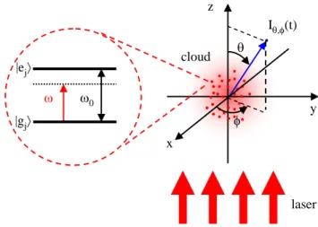
Even though it is possible to derive the equations de-scribing the evolution of coupled dipoles in the low excita-tion limit from classical equaexcita-tions, a quantum formalism is often conveniently used. We thus consider a set of N identical atoms interacting with a laser beam and vacuum modes (Fig. 1). Each atom j is a non-degenerate

two-level system, with ∣gj⟩ (resp. ∣ej⟩) labeling the ground

(resp. excited) state. The resonance frequency of the

atomic transition is ω0, the natural lifetime of the

ex-cited state is τ0 and the natural decay rate is Γ = 1/τ0.

The atoms are considered motionless and distributed at

random positions rj in a given distribution that models

the geometry of the sample. The laser beam is described by a classical monochromatic plane wave of amplitude

E0, wave vector k0 and frequency ω.

z I_,(t) laser cloud   x y ₀ |g_j |e_j 

FIG. 1. The physical system. A spherical Gaussian cloud of identical atoms interacts with a monochromatic plane wave with frequency ω and vacuum modes. The wave vector k0 of

the plane wave is set along the z direction. Each atom is a two-level system with resonance frequency ω0. The angles θ

and φ defines the spherical coordinates.

Following [21, 42] we write the coupled-dipole equa-tions in the scalar approximation as

˙ βj= (i∆ − Γ 2)βj− iΩ 2 e ik0⋅rj − Γ 2_j∑′_≠j eik0rjj′ ik0rjj′ βj′, (1)

where rjj′= ∣r_j−r_j′∣is the relative distance between the

atoms j and j′_{, Ω = dE}

0/̵h is the Rabi frequency

associ-ated to the laser drive, and ∆ = ω − ω0 is the laser

detun-ing from the atomic resonance. Here βj(t) are the

time-dependent amplitudes of dipoles j. Eq. (1) is valid for weak driving fields, i.e., the solution in the linear-optics regime. This amount to approximating the quantum so-lution to the first order in Ω, which is valid for s(∆) ≪ 1,

where s(∆) = 2Ω2/(Γ2+4∆2)is the saturation parameter.

We note that testing this assumption quantitatively, in particular in regard to the long-lived subradiant modes, would require a full quantum treatment [43]. In a

quan-tum framework, βj(t) can be considered as the optical

coherence of the atom j and the wave function of the atom ensemble reads

∣Ψ(t)⟩ = α(t) ∣G⟩ +

N

∑

j=1

βj(t) ∣j⟩ , (2)

where ∣G⟩ ≡ ∣g1...gN⟩is the ground state for all atoms and

∣j⟩ ≡ ∣g1...ej...gN⟩are the N single-atom excited states for each atom j.

B. Light scattered by the atomic cloud

The electric field at a position r far from the atomic

cloud is related to the atomic dipoles βj(t) by

E(r, t) ∝e −iω0(t−r/c) r N ∑ j=1 e−ik0r⋅rˆ j_β j(t) , (3)

where ˆr = r/r defines the direction of the detection from

the center of the atomic cloud. We thus obtain the

an-gular emitted intensity I ∝ ∣E∣2 by

I(ˆr, t) ∝ 1 r2 R R R R R R R R R R R N ∑ j=1 e−ik0ˆr⋅rj_β j(t) R R R R R R R R R R R 2 . (4)

In spherical coordinates, the emitted intensity in the direction (θ,φ) (see Fig. 1) can thus be written as

Iθ,φ(t) ∝ R R R R R R R R R R R N ∑ j=1 e−ik0fj(θ,φ)_β j(t) R R R R R R R R R R R 2 , (5)

where fj(θ, φ) = xjsin θ cos φ + yjsin θ sin φ + zjcos θ and

rj = (xj, yj, zj) are the coordinates of the atom j. We

thus first solve the coupled-dipole equations (1) and from

the solution of βj(t) we compute the angular- and

time-resolved scattered intensity using Eq. (5).

With a plane wave laser propagating along the z axis

with k0 =k0z and for an atomic cloud with revolutionˆ

symmetry around the z axis, we can integrate the angular intensity distribution along φ to obtain

Iθ(t) ∝∫ 2π 0 Iθ,φ(t)dφ =∫ 2π 0 R R R R R R R R R R R N ∑ j=1 e−ik0fj(θ,φ)_β j(t) R R R R R R R R R R R 2 dφ . (6) This integration along φ yields lower fluctuations for fi-nite numerical resolution. However, this procedure does not allow to study speckle-like fluctuations of the scat-tered light. Also, as we will see in section III D, for a laser drive with a phase profile which does not respect the rev-olution symmetry around the z axis, one cannot use the integration over φ to study super- and subradiance by a ‘phased’ excitation.

The total emitted power P (t) is the power emitted

by the atoms integrated over all directions: P (t) =

∫ I (r, t)dr with dr = r2sin θdrdθdφ. By substituting

Eq. (4), we obtain P (t) ∝_∫ π 0 ∫ 2π 0 R R R R R R R R R R R N ∑ j=1 e−ik0fj(θ,φ)_β j(t) R R R R R R R R R R R 2 sin θdθdφ. (7)

In this paper, we are mainly interested in the decay dynamics after the extinction of the driving laser and thus consider only times t ≥ 0, where t = 0 corresponds to the switch off of the driving field. For t ≥ 0, Ω = 0, one can show that Eq. (7) yields (see Appendix)

P (t) ∝ −d dt N ∑ j=1 ∣βj(t)∣ 2 , (8)

which can be interpreted as the energy transfer from the dipoles to the light. This simplified expression for the time-dependant total scattered light allows for faster nu-merics, convenient for some initial explorations, but as we show below, it is unable to provide the full scaling laws for superradiance, where angle-dependent effects can be prominent.

III. DECAY DYNAMICS FOR A SPHERICAL GAUSSIAN CLOUD

The atomic system is modeled as a spherical cloud with a Gaussian probability distribution ρ(rj) =ρ0e−∣rj∣

2_/2R2

, where R is the rms size of the cloud. The resonant

opti-cal thickness is b0 = 2N /(k0R)2 and the peak density

ρ0λ3 = (2π)3/2N /(k0R)3. Note that here we use the

definition of the optical depth for a scalar model, dif-ferent from what should be used in a vectorial model

[b(v)₀ = 3N /(k0R)2], where the polarization of the light

yields an on-resonant scattering cross section of 3λ2/2π.

The comparison to the optical depth in the experiment is furthermore different, as for atoms in a statistical mix-ture of the ground states, the on-resonant optical depth

is reduced by a degeneracy factor g = _{3(2F +1)}2F′+1 , which,

for the F = 2 → F′

= 3 transition of rubidium 87 used

in [30, 31] gives a reduction of the on-resonant optical depth of g ≈ 0.47.

Typical experimental values [30, 31] are λ ∼ 1µm,

N ∼ 109 and R ∼ 1 mm, yielding b0∼10 − 100 and ρ0λ3

∼10−2. With ρ0λ3≪1, the cloud is very dilute,

allow-ing to consider near-field effects as negligible. However,

it is very hard to simulate a cloud with 109 atoms on

available computers. So in practice we use N ∼ 103–104,

but we require b0 ∼10, in order to have similar optical

depths in the simulations as in the experiments. As a consequence of smaller N in the simulation, the

simu-lated density increases to ρ0λ3 ∼ 1–10. Moreover, the

computed intensities should be averaged for many differ-ent configurations of the positions of the atoms, in order to remove residual fluctuations, important for the small number of atoms used in simulations. In this article we have averaged over 100 realizations.

A. Impact of an exclusion volume

Our procedure for simulations consists in generating a spherical Gaussian cloud by choosing randomly the po-sitions of the N atoms from a Gaussian distribution of rms size R. However, as close atomic pairs may occur with such a random choice of positions, with a proba-bility increasing with the atomic density, and consider-ing that such pairs [16, 19, 39, 44] lead to strong two-body super- and subradiant decay absent in very dilute clouds, we choose to add an exclusion volume around each atom. After drawing the atomic positions in the

0 25 50 75 100 125 150 175 10−10 10−8 10−6 10−4 10−2 100 t / P(t) /P(0) without pairs with pairs single atom

FIG. 2. Comparison between the total emitted fluorescence for a spherical cloud with and without pairs (i.e., without and with an exclusion volume, respectively) for k0R ≈ 12.9,

b0 ≈7.55 and ρ0λ3 ≈4.6. The exclusion-volume condition is k0rjj′ <3 for the distance between all pairs of atoms j and j′

. The detuning is ∆ = 10Γ and the curves are obtained after averaging over 100 different configurations of the atomic positions.

cloud, we look for pairs of atoms with distance k0rjj′≤3

and change the corresponding positions until the condi-tion k0rjj′ > 3 if fulfilled for all pairs. This numerical

value for the exclusion volume corresponds to a distance where the two-body super- and subradiant decay rates, Γ2 = Γ [1 ± sin(k0rjj′)/k₀r_jj′], become close to

single-atom physics.

In order to illustrate the pair effect in the decay dy-namics, we plot in Fig. 2 the total scattered light (Eq. 8) for a cloud with and without using an exclusion volume. The cloud without pairs was generated from initial

tar-get parameters b0 = 10 and ρ0λ3= 7 for the Gaussian

distribution (with corresponding values of N = 633 and

k0R = 11.3). After the exclusion condition is fulfilled,

almost 50% of the N atoms had their position changed, however their distribution remains Gaussian with a good

approximation, but with a larger size: k0R increased to

12.9, implying that b0 and ρ0λ3 have to be recalculated.

That gives b0 = 7.55 and ρ0λ3=4.6. Note that this

in-crease of size comes along with introducing some corre-lation in the positions, which might induce some spuri-ous density effects. To compare this situation to a cloud without exclusion volume, we choose those final values for

b0 and ρ0λ3, only setting randomly the positions of the

atoms without the exclusion condition. As shown in Fig. (2), the presence of atomic pairs increases the subradiant amplitude at long times. This can be understood by the very long lifetimes of the two-atom subradiant state for very small distances.

B. Scaling of the super- and subradiance with b0

From decay curves similar as the one shown in Fig. 2, one can extract the super and subradiant decay rates Γsup, Γsub(or their associated time constant τsup=Γsup−1

, τsub= Γsub−1) by using an exponential fit in the

appro-priate range. For superradiance, the fit interval must be set at short time after the laser switch off, in order to get the first time constant. Here, we have used the fitting

interval t ∈ [0, 0.2]τ0. For subradiance, the fit interval

must be set long after the switch off of the laser, but, as discussed in the following (Sect. III D), the precise choice is somewhat arbitrary. Here we have chosen to fit the subradiant decay rate in the interval given by the rel-ative amplitude of the signal, Iθ(t)/Iθ(0) ∈ [10−4, 10−3],

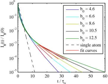
similar to what has been used in the experiment [30]. Ex-amples of decay curves and associated fits are shown in Fig. 3. Faster (superradiant) and slower (subradiant) de-cays compared to the single-atom decay are well visible.

We have chosen the emission angle θ = 45○_{for this}

illus-tration, but one can check that the decay is similar for other directions, except in the exact forward direction θ = 0, where a strong superradiant forward scattering lobe is present [11, 28, 45], and consequently the relative amplitude of the subradiant decay is much lower.

The duration of the pulse of the driving laser before switch off can also affect the results, as studied in detail in [35]. Here we consider only long-pulse excitation so that the steady-state is reached before the switch off.

We have numerically used a duration Tpulse=100τ0 and

0 10 20 30 40 50 60 10−5 10−4 10−3 10−2 10−1 100 t / τ 0 I θ (t) / I θ (0) b 0 = 4.6 b 0 = 6.6 b 0 = 8.6 b₀ = 10.5 b 0 = 12.5 single atom fit curves

FIG. 3. Decay of the scattered light in a direction θ = 45○

from the laser direction, computed from Eq. (6), for atomic samples of several b0 and constant density ρ0λ3=4.6. The laser detuning is ∆ = 10Γ. The red curves are exponential fits in the interval Iθ(t)/Iθ(0) ∈ [10−4, 10−3]that allow extracting the subradiant decay rate Γsub. A similar fit (not showed) is

done in the interval t ∈ [0, 0.2]τ0 to extract the superradiant

decay rate Γsup. The black dashed line is the decay curve for

0 2 4 6 8 10 12 14 0 1 2 3 4 b₀ (a) 0 2 4 6 8 10 12 14 0 1 2 3 4 5 6 7 8 9 b₀ (b)

FIG. 4. Cooperative decay rates Γsup (a) and τsub=Γsub−1(b)

as a function of the resonant optical depth b0 for different

densities ρ0λ3=0.5 (red ○), 0.9 (blue ◇), 2.5 (green +), 3.7 (yellow ∗), 4.6 (magenta ×) and 5.3 (black ◻). The decay rates are obtained by fitting decay curves similar as those in Fig. 3, computed with a laser excitation at a large detuning ∆ = 10Γ and a long pulse in order to reach the steady state.

have checked that starting from the steady-state solution before switching off the laser does not modify the results. The behavior of the super- and subradiant decay rates as a function of the parameters of the cloud (atom num-ber, size, optical depth or density) has been the subject of extensive discussions. In the case of a low-density sam-ple driven at large detuning, the collective steady state is essentially the timed-Dicke state [8, 11, 46]. The

corre-sponding superradiant decay rate Γsup has been

analyti-cally computed for various geometries [21, 47–51] and it has been shown that it is proportional to the resonant

op-tical depth b0. Based on numerical investigations, it has

been argued that the same apply for subradiance, with

a characteristic time τsub evolving linearly with b0 [52].

This result has been checked numerically and experimen-tally in [30, 53]. It has been actually showed that the full

decay curves depends only on b0 in this regime [9].

All previous calculations and simulations, however, ap-ply to the total decay rate of the collective state, which is mainly dominated by the forward scattering lobe. In

Fig. 4 we present the superradiant decay rate Γsup and

subradiant decay time τsubcomputed from the scattered

light at θ = 45○ _{as a function of b}

0 for several densities,

following an excitation to the steady state with a large detuning ∆ = 10Γ. The chosen angle is close to the ex-perimental configuration of [30, 31]. The computation

is done for several densities, in order to check whether the density plays any role. The results of the simulations show that the density plays only a marginal role, inducing a small shift of the superradiant decay rate (Fig. 4a) and not affecting the subradiant one (Fig. 4b). This resid-ual density effect might come from the correlations intro-duced by the exclusion volume condition and should thus be absent at the lower densities of the experiments. The main trend is clearly the linear evolution of the superra-diant decay rate and subrasuperra-diant time constant, following

Γsup= (1 + αb0)Γ , (9)

τsub= (1 + βb0)τ0. (10)

Linear fitting the low-density data gives α ≈ 0.21 and β ≈ 0.53. For comparison, the only available analytical results is for the total decay rate of the time-Dicke state, which gives α = 1/8 for a Gaussian cloud [42]. We indeed recover this scaling for forward scattering, but superradi-ance is “stronger” for light scattered off-axis, as already discussed in [31]. Note that we do not expect any quan-titative agreement with the experiments because of the complex multilevel structure of the atoms used in the experiments.

C. Angular dependance of super- and subradiance

As already mentioned, the decay dynamics in general depends on the scattering angle (Eq. 6). The most promi-nent feature of the angular dependence is the forward scattering lobe [11, 45]. It is visible in steady state but, as it is mainly superradiant, it also affects the temporal dynamics, with, in particular, a lower relative weight of subradiant decay in the forward direction and a slightly different slope α (Eq. 9) for the superradiant decay [31]. An extensive study of the superradiant decay rate as a function of the scattering angle has recently been pre-sented, showing a complicated dependency near the for-ward lobe [35]. It also depends on the detuning of the exciting laser.

In Fig. 5(a) we summarize these findings on the super-radiant decay rate as a function of the scattering angle for near-resonance and detuned excitation, and we also show the behavior of the subradiant decay in Fig. 5(b). The

resonant optical depth is fixed, b0 =8.55. At large

de-tuning, the superradiant decay rate Γsup is significantly

larger off axis than exactly on axis, which is a nonin-tuitive feature. Except very close to the forward lobe,

where Γsupevolves a lot with the angle (not shown here,

see [35]), Γsup hardly evolves everywhere else. On

reso-nance, on the contrary, superradiance is visible only in

the forward direction, and Γsup<Γ off axis, which means

that superradiance is suppressed and that the light es-cape rate is slowed down by multiple scattering [54]. Al-though the collective state is different from the timed-Dicke state in this situation [8], and more generally su-perradiant modes are much less populated near resonance

0 30 60 90 120 150 180 0 0.5 1 1.5 2 2.5 3 θ (°) Γ sup / Γ (a) 0 30 60 90 120 150 180 0 1 2 3 4 5 6 7 8 9 θ (°) τ sub / τ 0 (b) ∆ = 0 ∆ = 10Γ

FIG. 5. Cooperative decay rates Γsup (a) and τsub (b) as a function of the detection angle θ measured from the laser axis,

where θ = 0 is the forward direction and θ = 180○

is the backscattering direction. Data were calculated for on-resonance (red) and far-detuned (blue) excitation, for a sample with fixed density ρ0λ3=4.6 and b0=8.55. In (a), superradiance is suppressed on-resonance except in the forward direction. Off-resonance, it is faster off-axis (θ ≠ 0) than on-axis (θ = 0). In (b), subradiance is isotropic for all detunings and directions. The fitting range of the subradiant decay has been set to a lower value for the point at θ = 0 in order to take into account the lower relative amplitude of subradiance due to the forward superradiant lobe.

[46], the forward superradiant lobe is still preserved be-cause it comes from the diffracted light on the edge of the cloud when driven by a plane wave. For subradiance,

we do not see any significant variation of τsub with the

emission angle, confirming initial intuition that subradi-ance is on average isotropic [30, 52]. The relative ampli-tude of the subradiant decay is however much smaller at θ = 0 because of the dominant forward superradiant lobe. The slightly slower decay at resonance is due to multiple scattering, which contributes to slowing down the de-cay [54]. The precise interplay between subradiance and multiple scattering near resonance is the subject of stud-ies in progress.

D. Long-time limit

As mentioned at the beginning, the fitting interval for subradiance is somewhat arbitrary and the subradiant decay time that can be measured in an experiment is related to the noise level below which the decay is not measurable. It is thus interesting to look if the decay rate still evolves at very late times, even if those times are not accessible experimentally. From the numerical decay curves, we can compute the instantaneous decay rate

Γ(t) = −d

dt[ln P (t)] , (11)

here defined for the total scattered light (Eq. 7).

In Fig. 6 we show Γ(t) for ∆ = 10Γ and different

val-ues of b0. We find that the decay rates still evolve long

after the switch off, until it eventually reaches a constant

value at very long time, here t ≥ 600τ0. We have checked

that this does not depend on the duration of the

excit-ing pulse. The final value of Γ(t) corresponds to the

smallest real part of the eigenvalue spectrum (see [46]), which is very sensitive to the configuration of the po-sitions. Moreover, the population of the corresponding mode can be negligible, which means that the signal is

101 102 103 10−1 100 t / τ 0 Γ (t) / Γ b 0 = 4.6 b 0 = 6.6 b 0 = 8.6 b 0 = 10.5 b 0 = 12.5

FIG. 6. Temporal decay rates Γ(t) calculated from the total fluorescence (Eq. 8), for several b0, with ρ0λ3=4.6 and ∆ = 10Γ. The decay rates still evolve even for very long times, becoming completely constant for t ≥ 600τ0 after the

(b) (a)

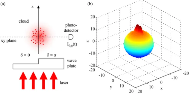
FIG. 7. Phased cloud. (a) The cloud is excited by a laser propagating along the z axis, which goes through a wave plate such as the half space y > 0 of the cloud is excited with a phase shift of δ = π compared to the atoms in the half space y < 0. The detector measures the intensity Iθ,φ(t) computed from Eq. (5). (b) Emission diagram in the steady state for the phased cloud,

for b0=8.55, ρ0λ3=4.6 and ∆ = 10Γ. The single forward lobe, characteristic of superradiance with a plane wave (without phase shift), is divided into two components for the “phased” excitation. The emission diagram is isotropic in other directions.

far below the detection threshold of any realistic exper-iment. The long-time limit of Γ(t) is thus not relevant from an experimental point of view. On the other hand, this problem shows that we lack a rigorous definition of the subradiant decay rate, and we have to rely on empir-ical definitions to measure or numerempir-ically evaluate it.

IV. SUBRADIANCE IN A PHASED CLOUD

Subradiance is hard to detect experimentally because of its low relative level in the decay dynamics, on the

or-der of 10−3[30], which limits the prospect of using

subra-diant states for quantum information processing, metrol-ogy, or transport experiments [41, 55–59]. Finding a way to selectively populate the subradiant states, or at least to enhance their relative weight, is thus a relevant chal-lenge.

Inspired by [41], in this section we analyze the decay dynamics of what we call a phased cloud (Fig. 7a). This is an atomic cloud where one half side is driven with a phase shift of δ = π compared to the atoms in the other half (δ = 0). This set-up can be experimentally realized by making the incoming laser to go through a wave plate of different thickness. Then, after the laser extinction, the scattered light is detected in the direction orthogonal to the phase step.

For the simulations, the driving laser is set along the z-axis and the phase shifter is placed such that the atoms in the half space y > 0 are driven by the laser with the

phase k0zj+π in Eq. (1), while the atoms in the half space

y < 0 are driven with the phase k0zj as previously. As

the phased-cloud system is not symmetric with respect to the z-axis, we use Eq. (5) to compute the scattered light in a given direction θ, φ. Fig. 7b shows the emission diagram of the phased cloud in the steady state. The main effect of the phase step is to divide the forward emission into two lobes. This is due to the destructive interference between the light emitted by the atoms in the two different half spaces. A similar idea, controlling the direction of the main diffraction lobe via the phase of the driven atoms, has been discussed in [60].

The remarkable property of this phased cloud is the de-cay dynamics for directions orthogonal to the laser axis

(θ = 90○_{). Fig. 8(a) compares the scattered intensity for}

the phased excitation and the standard excitation, i.e., without phase shifter (“normal” excitation). As previ-ously, the data are normalized to the steady-state values before switch off, which are similar in both cases. How-ever, after some decay time, the signal obtained with the phased excitation is significantly higher. This means that the relative weight of subradiance is enhanced by a factor

∼6 − 8 [Fig. 8(b)], which is a significant improvement for

experiments. It also shows that subradiance is sensitive to the phase of the laser, which is a marked difference with radiation trapping [54], and thus stresses that this is a coherent effect.

This improvement obtained with a very simple phase profile for the incident laser shows that there should be possible to enhance the population of the subradiant states by engineering the phase or intensity or temporal profile of the exciting laser.

0 10 20 30 40 50 10−6 10−5 10−4 10−3 10−2 10−1 100 (a) normal excitation phased excitation 0 50 100 150 200 0 2 4 6 8 10 I phased /I normal (b)

FIG. 8. (a) Comparison between the normal and phased cloud for the decay dynamics. The parameters of the sample are b0 =8.55, ρ0λ3=4.6 and the laser detuning is ∆ = 10Γ. Superradiance is almost completely suppressed and the rel-ative amplitude of subradiance is increased, while the decay rate is conserved. Here the scattered intensity is calculated at θ = 90○

, φ = 90○

(see Fig. 7), but the result is similar for all φ. (b) Ratio between the scattered light from the phased and normal cloud, during the decay, as computed in (a). The phased excitation increases the relative amplitude of subradi-ance by a factor ∼ 6–8.

V. SUMMARY

In this article, we have reported a detailed numerical investigation on the decay dynamics for a dilute

spher-ical Gaussian cloud of N particles, using the

coupled-dipole equations. We have discussed the effect of

us-ing an exclusion-volume condition avoidus-ing pairs of close atoms, in order to better simulate the low-density regime in which some experiments are performed [30, 31]. It was shown that the superradiant decay rate scales linearly

with the resonant optical depth b0. On the contrary, the

subradiant decay rate, although defined with some

arbi-trary considerations, is inversely proportional to b0. We

have also shown that while the superradiant decay rate is significatively different for the light scattered on axis and off axis, the subradiant decay rate is isotropic. Fi-nally, the decay dynamics of a sample driven by a laser with a 0 − π phase profile was studied and it was shown that this configuration increases significantly the relative weight of subradiance detected in some directions. This paves the way for the development of even more involved and efficient way to selectively populate the subradiant states, which is promising for their future use in various fields, for instance for quantum information processing, metrology, or transport experiments [41, 55–59].

ACKNOWLEDGEMENTS

We thank Marlan Scully for insightful suggestions

dur-ing the 2017 PQE Conference and Carlos M´aximo,

Ro-main Bachelard, Philippe Courteille, and Nicolas Piovella for useful discussions about the coupled-dipole model and simulation methods.

FUNDING

We acknowledge financial support from the French Agency ANR (project LOVE, No. ANR-14-CE26-0032) and the Brazilian CAPES Foundation.

[1] R. H. Dicke, “Coherence in spontaneous radiation pro-cesses,” Phys. Rev. 93, 99–110 (1954).

[2] R. Friedberg, S. R. Hartmann, and J. T. Manassah, “Frequency shifts in emission and absorption by reso-nant systems of two-level atoms,” Phys. Rep. 7, 101–179 (1973).

[3] M. S. Feld and J. C. MacGillivray, “Coherent nonlinear optics. recent advances,” (Springer, Berlin, 1980) Chap. Superradiance, pp. 7–57.

[4] M. Gross and S. Haroche, “Superradiance: an essay on the theory of collective spontaneous emission,” Phys. Rep. 93, 301–396 (1982).

[5] A. Lagendijk and B. A. van Tiggelen, “Resonant multiple scattering of light,” Phys. Rep. 270, 143–215 (1996). [6] G. Labeyrie, “Coherent transport of light in cold atoms,”

Mod. Phys. Lett. B 22, 73–99 (2008).

[7] J. T. Manassah, “Cooperative radiation from atoms in different geometries: decay rate and frequency shift,” Adv. Opt. Photon. 4, 108–156 (2012).

[8] T. Bienaim´e, R. Bachelard, P. W. Courteille, N. Piovella, and R. Kaiser, “Cooperativity in light scattering by cold atoms,” Fortschr. Phys. 61, 377–392 (2013).

[9] W. Guerin, M. T. Rouabah, and R. Kaiser, “Light inter-acting with atomic ensembles: collective, cooperative and mesoscopic effects,” J. Mod. Opt. 64, 895–907 (2017).

[10] D. V. Kupriyanov, I. M. Sokolov, and M. D. Havey, “Mesoscopic coherence in light scattering from cold, op-tically dense and disordered atomic systems,” Phys. Rep. 671, 1–60 (2017).

[11] M. O. Scully, E. S. Fry., C. H. Raymond Ooi, and K. W´odkiewicz, “Directed spontaneous emission from an extended ensemble of N atoms: Timing is everything,” Phys. Rev. Lett. 96, 010501 (2006).

[12] M. O. Scully and A. A. Svidzinsky, “The super of super-radiance,” Science 325, 1510–1511 (2009).

[13] F. Fr¨owis, P. C. Strassmann, A. Tiranov, C. Gut, J. Lavoie, N. Brunner, F. Bussi`eres, M. Afzelius, and N. Gisin, “Experimental certification of millions of gen-uinely entangled atoms in a solid,” arXiv:1703.04704 (2017).

[14] E. Akkermans, A. Gero, and R. Kaiser, “Photon local-ization and Dicke superradiance in atomic gases,” Phys. Rev. Lett. 101, 103602 (2008).

[15] M. Rusek, A. Or lowski, and J. Mostowski, “Localization of light in three-dimensional random dielectric media,” Phys. Rev. E 53, 4122–4130 (1996).

[16] M. Rusek, J. Mostowski, and A. Or lowski, “Random green matrices: From proximity resonances to Anderson localization,” Phys. Rev. A 61, 022704 (2000).

[17] F. A. Pinheiro, M. Rusek, A. Orlowski, and B. A. van Tiggelen, “Probing Anderson localization of light via de-cay rate statistics,” Phys. Rev. E 69, 026605 (2004). [18] S. E. Skipetrov and I. M. Sokolov, “Absence of

Ander-son localization of light in a random ensemble of point scatterers,” Phys. Rev. Lett. 112, 023905 (2014). [19] L. Bellando, A. Gero, E. Akkermans, and R. Kaiser,

“Cooperative effects and disorder: A scaling analysis of the spectrum of the effective atomic Hamiltonian,” Phys. Rev. A 90, 063822 (2014).

[20] S. E. Skipetrov, “Finite-size scaling analysis of localiza-tion transilocaliza-tion for scalar waves in a three-dimensional ensemble of resonant point scatterers,” Phys. Rev. B 94, 064202 (2016).

[21] Ph. W. Courteille, S. Bux, E. Lucioni, K. Lauber, T. Bi-enaim´e, R. Kaiser, and N. Piovella, “Modification of ra-diation pressure due to cooperative scattering of light,” Eur. Phys. J. D. 58, 69–73 (2010).

[22] T. Bienaim´e, S. Bux, E. Lucioni, Ph. W. Courteille, N. Piovella, and R. Kaiser, “Observation of cooperative radiation pressure in presence of disorder,” Phys. Rev. Lett. 104, 183602 (2010).

[23] J. Chab´e, M. T. Rouabah, L. Bellando, T. Bienaim´e, N. Piovella, R. Bachelard, and R. Kaiser, “Coherent and incoherent multiple scattering,” Phys. Rev. A 89, 043833 (2014).

[24] R. Bachelard, N. Piovella, W. Guerin, and R. Kaiser, “Collective effects in the radiation pressure force,” Phys. Rev. A 94, 033836 (2016).

[25] G. Labeyrie, F. de Tomasi, J.-C. Bernard, C. A. M¨uller, C. Miniatura, and R. Kaiser, “Coherent backscattering of light by cold atoms,” Phys. Rev. Lett. 83, 5266–5269 (1999).

[26] C. C. Kwong, T. Yang, , D. Delande, R. Pierrat, and D. Wilkowski, “Cooperative emission of a pulse train in an optically thick scattering medium,” Phys. Rev. Lett. 115, 223601 (2015).

[27] S. Jennewein, M. Besbes, N. J. Schilder, S. D. Jenkins, C. Sauvan, J. Ruostekoski, J.-J. Greffet, Y. R. P. Sortais, and A. Browaeys, “Coherent scattering of near-resonant

light by a dense microscopic cold atomic cloud,” Phys. Rev. Lett. 116, 233601 (2016).

[28] S. J. Roof, K. J. Kemp, M. D. Havey, and I. M. Sokolov, “Observation of single-photon superradiance and the co-operative Lamb shift in an extended sample of cold atoms,” Phys. Rev. Lett. 117, 073003 (2016).

[29] J. Pellegrino, R. Bourgain, S. Jennewein, Y. R. P. Sor-tais, A. Browaeys, S. D. Jenkins, and J. Ruostekoski, “Observation of suppression of light scattering induced by dipole-dipole interactions in a cold-atom ensemble,” Phys. Rev. Lett. 113, 133602 (2014).

[30] W. Guerin, M. O. Ara´ujo, and R. Kaiser, “Subradiance in a large cloud of cold atoms,” Phys. Rev. Lett. 116, 083601 (2016).

[31] M. O. Ara´ujo, I. Kreˇsi´c, R. Kaiser, and W. Guerin, “Su-perradiance in a large cloud of cold atoms in the linear-optics regime,” Phys. Rev. Lett. 117, 073002 (2016). [32] T. Jonckheere, C. A. M¨uller, R. Kaiser, Ch. Miniatura,

and D. Delande, “Multiple scattering of light by atoms in the weak localization regime,” Phys. Rev. Lett. 85, 4269 (2000).

[33] S. Roof, K. Kemp, M. D. Havey, I. M. Sokolov, and D. V. Kupriyanov, “Microscopic lensing by a dense, cold atomic sample,” Opt. Lett. 40, 1137 (2015).

[34] S. D. Jenkins, J. Ruostekoski, J. Javanainen, S. Jen-newein, R. Bourgain, J. Pellegrino, Y. R. P. Sortais, and A. Browaeys, “Collective resonance fluorescence in small and dense atom clouds: Comparison between theory and experiment,” Phys. Rev. A 94, 023842 (2016).

[35] A. S. Kuraptsev, I. Sokolov, and M. D. Havey, “Angular distribution of single photon superradiance in a dilute and cold atomic ensemble,” arXiv:1701.07503 (2017). [36] J. Javanainen, J. Ruostekoski, B. Vestergaard, and M. R.

Francis, “One-dimensional modeling of light propagation in dense and degenerate samples,” Phys. Rev. A 59, 649 – 666 (1999).

[37] A. A. Svidzinsky, J.-T. Chang, and M. O. Scully, “Co-operative spontaneous emission of N atoms: Many-body eigenstates, the effect of virtual Lamb shift processes, and analogy with radiation of N classical oscillators,” Phys. Rev. A 81, 053821 (2010).

[38] E. Abrahams, P. W. Anderson, D. C. Licciardello, and T. V. Ramakrishnan, “Scaling theory of localization: ab-sence of quantum diffusion in two dimensions,” Phys. Rev. Lett. 4, 673–676 (1979).

[39] S. E. Skipetrov and A. Goetschy, “Eigenvalue distribu-tions of large Euclidean random matrices for waves in random media,” J. Phys. A: Math. Theor. 44, 065102 (2011).

[40] M. Hebenstreit, B. Kraus, L. Ostermann, and H. Ritsch, “Subradiance via entanglement in atoms with several in-dependent decay channels,” Phys. Rev. Lett. 118, 143602 (2017).

[41] M. O. Scully, “Single photon subradiance: Quantum control of spontaneous emission and ultrafast readout,” Phys. Rev. Lett. 115, 243602 (2015).

[42] T. Bienaim´e, M. Petruzzo, D. Bigerni, N. Piovella, and R. Kaiser, “Atom and photon measurement in coopera-tive scattering by cold atoms,” J. Mod. Opt. 58, 1942– 1950 (2011).

[43] L. Pucci, A. Roy, T. Santiago do Espirito Santo, R. Kaiser, M. Kastner, and R. Bachelard, “Quantum ef-fects in the cooperative scattering of light by cold atomic clouds,” arXiv:1701.04061 (2017).

[44] R. G. DeVoe and R. G. Brewer, “Observation of su-perradiant and subradiant spontaneous emission of two trapped ions,” Phys. Rev. Lett. 76, 2049–2052 (1996). [45] S. L. Bromley, B. Zhu, M. Bishof, X. Zhang, T.

Both-well, J. Schachenmayer, T. L. Nicholson, R. Kaiser, S. F. Yelin, M. D. Lukin, A. M. Rey, and J. Ye, “Collective atomic scattering and motional effects in a dense coher-ent medium,” Nat. Commun. 7, 11039 (2016).

[46] W. Guerin and R. Kaiser, “Population of collective modes in light scattering by many atoms,” arXiv:1795405 (2017).

[47] I. E. Mazets and G. Kurizki, “Multiatom cooperative emission following single-photon absorption: Dicke-state dynamics,” J. Phys. B: At. Mol. Opt. Phys. 40, F105– F112 (2007).

[48] A. A. Svidzinsky, J.-T. Chang, and M. O. Scully, “Dy-namical evolution of correlated spontaneous emission of a single photon from a uniformly excited cloud of N atoms,” Phys. Rev. Lett. 100, 160504 (2008).

[49] A. A. Svidzinsky and J.-T. Chang, “Cooperative spon-taneous emission as a many-body eigenvalue problem,” Phys. Rev. A 77, 043833 (2008).

[50] R. Friedberg and J. T. Manassah, “Analytic expressions for the initial cooperative decay rate and cooperative Lamb shift for a spherical sample of two-level atoms,” Phys. Lett. A 374, 1648–1659 (2010).

[51] S. Prasad and R. J. Glauber, “Coherent radiation by a spherical medium of resonant atoms,” Phys. Rev. A 82, 063805 (2010).

[52] T. Bienaim´e, N. Piovella, and R. Kaiser, “Controlled Dicke subradiance from a large cloud of two-level sys-tems,” Phys. Rev. Lett. 108, 123602 (2012).

[53] In the Fig. 1 of the Supplemental Material of [30], the b0

-axis has not been correctly rescaled to take into account the increase of size induced by the exclusion volume, as explained in Sect. III A.

[54] G. Labeyrie, E. Vaujour, C. A. M¨uller, D. Delande, C. Miniatura, D. Wilkowski, and R. Kaiser, “Slow dif-fusion of light in a cold atomic cloud,” Phys. Rev. Lett. 91, 223904 (2003).

[55] L. Ostermann, H. Ritsch, , and C. Genes, “Protected state enhanced quantum metrology with interacting two-level ensembles,” Phys. Rev. Lett. 111, 123601 (2013). [56] D.-W. Wang H. Cai, A. A. Svidzinsky, S.-Y. Zhu, and

M. O. Scully, “Symmetry-protected single-photon subra-diance,” Phys. Rev. A 93, 053804 (2016).

[57] G. Facchinetti, S. D. Jenkins, and J. Ruostekoski, “Stor-ing light with subradiant correlations in arrays of atoms,” Phys. Rev. Lett. 117, 243601 (2016).

[58] A. Asenjo-Garcia, M. Moreno-Cardoer, A. Albrecht, H. J. Kimble, and D. E. Chang, “Exponential improve-ment in photon storage fidelities using subradiance and selective radiance in atomic arrays,” arXiv:1703.03382 (2017).

[59] G. L. Celardo, M. Angeli, and R. Kaiser, “Localization of light in subradiant Dicke states,” arXiv:1702.04506 (2017).

[60] C. E. M´aximo, R. Kaiser, Ph. W. Courteille, and R. Bachelard, “The atomic lighthouse effect,” J. Opt. Soc. Am. A 31, 2511–2517 (2014).

[61] J. D. Jackson, Classical Electrodynamics, 3rd ed. (Wiley, New York, 1999).

Appendix A: Proof of Equation (8)

The equivalence of the Eqs. (7) and (8) is verified by showing that both are proportional to

I = ∑ j ∑ j′ sin(k0rjj′) k0rjj′ βjβ∗j′. (A1)

For simplicity we have dropped the j, j′

=1, ..., N in the summation.

Let us to start with Eq. (7). We rewrite it as P (t) ∝ ∑ j ∑ j′ ∫ 2π 0 ∫ π 0 e−ik0r⋅(rˆ j−rj′)_β jβj∗′sin θdθdφ . (A2)

By choosing a coordinate frame such that ˆr ⋅ (rj−rj′) =

rjj′cos θ [61], and noting that the integral over φ gives

2π, we have P (t) ∝ 2π ∑ j ∑ j′ βjβj∗′_∫ π 0

e−ik0rjj′cos θ_{sin θdθ}

= 2π ∑ j ∑ j′ βjβ ∗ j′_∫ 1 −1 e−ik0rjj′u_du = 4π ∑ j ∑ j′ sin(k0rjj′) k0rjj′ βjβj∗′, (A3)

i.e., proportional to Eq. (A1). Note that Eq. (A3) is valid for all t and not only during the decay (t > 0).

Now we turn to Eq. (8). We start by expanding the derivative in the right-hand side by using the Kronecker delta: f (t) ≡ −d dt∑_j ∣βj(t)∣ 2 = −d dt∑_j ∑_j′ βjβj∗′δjj′ = − ∑ j ∑ j′ δjj′( ˙β_jβ ∗ j′+βjβ˙j∗′). (A4)

The terms ˙βjare replaced by the coupled-dipole equation

(1) and its complex conjugate, rewritten with the term

(−Γ/2)βj absorbed into the summation, i.e.,

˙ βj=i∆βj− iΩ 2 e ik0⋅rj − Γ 2 ∑_j′ Vjj′β_j′. (A5)

After the substitutions, we have f (t) = − ∑ j ∑ j′ δjj′([i∆β_j− iΩ 2 e ik0⋅rj − Γ 2 ∑m Vjmβm]β_j∗′ +βj [−i∆βj∗′+ iΩ 2 e −ik0⋅rj′₋Γ 2∑n V∗ j′_nβ ∗ n]) = Γ 2∑_j ∑_j′ δjj′_(∑ m Vjmβmβj∗′+ ∑ n V∗ nj′βjβn∗) + iΩ 2 ∑_j (e ik0⋅rj_β∗ j −c.c.) = Γ 2∑_j ∑_j′ (Vjj′+V_jj∗′)βjβj∗′ − iΩ 2 ∑_j (e −ik0⋅rj_β j−c.c.) (A6)

The first term is proportional to Eq. (A1) after sub-stituting Vjj′ = eik0rjj′_/(ik0rjj′) and noting that it is

symmetric to the exchange j ⇆ j′_{. Furthermore, from}

Eq. (A3), it is also equal to the total emitted power P (t).

Thus, we rewrite Eq. (A6) as

P (t) ∝ −d dt∑_j ∣βj(t)∣ 2 + iΩ 2 ∑_j (e −ik0⋅rj_β j−c.c.) (A7) for all t.

When the driving laser is switched off, Ω = 0 and Eq. (A7) yields to Eq. (8), valid during the decay.