Search for the rare decay Bs->mumu

(1)

arXiv:1301.4507v1 [hep-ex] 18 Jan 2013

Search for the rare decay B

0

s

→

µ

+

_µ

₋

V.M. Abazov,32 _{B. Abbott,}67 _{B.S. Acharya,}26_{M. Adams,}46 _{T. Adams,}44 _{G.D. Alexeev,}32 _{G. Alkhazov,}36 A. Altona_,56 _{A. Askew,}44 _{S. Atkins,}54 _{K. Augsten,}7 _{C. Avila,}5 _{F. Badaud,}10 _{L. Bagby,}45 _{B. Baldin,}45 D.V. Bandurin,44_{S. Banerjee,}26 _{E. Barberis,}55 _{P. Baringer,}53 _{J.F. Bartlett,}45 _{U. Bassler,}15_{V. Bazterra,}46 A. Bean,53 _{M. Begalli,}2_{L. Bellantoni,}45_{S.B. Beri,}24 _{G. Bernardi,}14 _{R. Bernhard,}19_{I. Bertram,}39 _{M. Besan¸con,}15 R. Beuselinck,40_{P.C. Bhat,}45_{S. Bhatia,}58_{V. Bhatnagar,}24_{G. Blazey,}47_{S. Blessing,}44 _{K. Bloom,}59 _{A. Boehnlein,}45

D. Boline,64 _{E.E. Boos,}34 _{G. Borissov,}39 _{A. Brandt,}70 _{O. Brandt,}20 _{R. Brock,}57 _{A. Bross,}45 _{D. Brown,}14 X.B. Bu,45 _{M. Buehler,}45 _{V. Buescher,}21 _{V. Bunichev,}34 _{S. Burdin}b_,39 _{C.P. Buszello,}38_{E. Camacho-P´erez,}29

B.C.K. Casey,45_{H. Castilla-Valdez,}29 _{S. Caughron,}57_{S. Chakrabarti,}64 _{D. Chakraborty,}47 _{K.M. Chan,}51 A. Chandra,72 _{E. Chapon,}15_{G. Chen,}53 _{S.W. Cho,}28 _{S. Choi,}28 _{B. Choudhary,}25 _{S. Cihangir,}45 _{D. Claes,}59 J. Clutter,53 _{M. Cooke,}45_{W.E. Cooper,}45 _{M. Corcoran,}72_{F. Couderc,}15_{M.-C. Cousinou,}12 _{D. Cutts,}69 _{A. Das,}42

G. Davies,40_{S.J. de Jong,}30, 31 _{E. De La Cruz-Burelo,}29 _{F. D´eliot,}15_{R. Demina,}63 _{D. Denisov,}45 _{S.P. Denisov,}35 S. Desai,45 _{C. Deterre}d_,20 _{K. DeVaughan,}59_{H.T. Diehl,}45 _{M. Diesburg,}45 _{P.F. Ding,}41 _{A. Dominguez,}59_{A. Dubey,}25

L.V. Dudko,34 _{A. Duperrin,}12 _{S. Dutt,}24 _{A. Dyshkant,}47 _{M. Eads,}47_{D. Edmunds,}57_{J. Ellison,}43 _{V.D. Elvira,}45 Y. Enari,14_{H. Evans,}49 _{V.N. Evdokimov,}35_{L. Feng,}47 _{T. Ferbel,}63_{F. Fiedler,}21 _{F. Filthaut,}30, 31 _{W. Fisher,}57 H.E. Fisk,45 _{M. Fortner,}47 _{H. Fox,}39_{S. Fuess,}45_{P. H. Garbincius,}45 _{A. Garcia-Bellido,}63 _{J.A. Garc´ıa-Gonz´alez,}29

G.A. Garc´ıa-Guerrac_,29 _{V. Gavrilov,}33 _{W. Geng,}12, 57 _{C.E. Gerber,}46 _{Y. Gershtein,}60 _{G. Ginther,}45, 63 G. Golovanov,32 _{P.D. Grannis,}64 _{S. Greder,}16 _{H. Greenlee,}45 _{G. Grenier,}17 _{Ph. Gris,}10 _{J.-F. Grivaz,}13 A. Grohsjeand_,15_{S. Gr¨}_unendahl,45 _{M.W. Gr¨}_unewald,27_{T. Guillemin,}13 _{G. Gutierrez,}45 _{P. Gutierrez,}67_{J. Haley,}55 L. Han,4 _{K. Harder,}41 _{A. Harel,}63_{J.M. Hauptman,}52 _{J. Hays,}40 _{T. Head,}41_{T. Hebbeker,}18_{D. Hedin,}47 _{H. Hegab,}68

A.P. Heinson,43 _{U. Heintz,}69 _{C. Hensel,}20_{I. Heredia-De La Cruz,}29 _{K. Herner,}56 _{G. Hesketh}f_,41 _{M.D. Hildreth,}51 R. Hirosky,73_{T. Hoang,}44 _{J.D. Hobbs,}64_{B. Hoeneisen,}9 _{J. Hogan,}72 _{M. Hohlfeld,}21 _{I. Howley,}70 _{Z. Hubacek,}7, 15 V. Hynek,7 _{I. Iashvili,}62 _{Y. Ilchenko,}71 _{R. Illingworth,}45_{A.S. Ito,}45 _{S. Jabeen,}69 _{M. Jaffr´e,}13 _{A. Jayasinghe,}67

M.S. Jeong,28_{R. Jesik,}40 _{P. Jiang,}4_{K. Johns,}42 _{E. Johnson,}57 _{M. Johnson,}45 _{A. Jonckheere,}45_{P. Jonsson,}40 J. Joshi,43 _{A.W. Jung,}45 _{A. Juste,}37 _{E. Kajfasz,}12_{D. Karmanov,}34_{I. Katsanos,}59 _{R. Kehoe,}71_{S. Kermiche,}12 N. Khalatyan,45_{A. Khanov,}68 _{A. Kharchilava,}62 _{Y.N. Kharzheev,}32 _{I. Kiselevich,}33 _{J.M. Kohli,}24_{A.V. Kozelov,}35

J. Kraus,58_{A. Kumar,}62 _{A. Kupco,}8 _{T. Kurˇca,}17 _{V.A. Kuzmin,}34 _{S. Lammers,}49_{P. Lebrun,}17 _{H.S. Lee,}28 S.W. Lee,52 _{W.M. Lee,}44 _{X. Lei,}42 _{J. Lellouch,}14_{D. Li,}14 _{H. Li,}73 _{L. Li,}43 _{Q.Z. Li,}45_{J.K. Lim,}28 _{D. Lincoln,}45 J. Linnemann,57V.V. Lipaev,35 R. Lipton,45 H. Liu,71 Y. Liu,4A. Lobodenko,36M. Lokajicek,8 R. Lopes de Sa,64 R. Luna-Garciag_,29_{A.L. Lyon,}45_{A.K.A. Maciel,}1_{R. Maga˜}_na-Villalba,29_{S. Malik,}59_{V.L. Malyshev,}32 _{J. Mansour,}20

J. Mart´ınez-Ortega,29 _{R. McCarthy,}64 _{C.L. McGivern,}41 _{M.M. Meijer,}30, 31 _{A. Melnitchouk,}45 _{D. Menezes,}47 P.G. Mercadante,3 _{M. Merkin,}34 _{A. Meyer,}18_{J. Meyer}j_,20 _{F. Miconi,}16 _{N.K. Mondal,}26_{M. Mulhearn,}73 _{E. Nagy,}12

M. Naimuddin,25 _{M. Narain,}69 _{R. Nayyar,}42_{H.A. Neal,}56 _{J.P. Negret,}5 _{P. Neustroev,}36 _{H.T. Nguyen,}73 T. Nunnemann,22 _{J. Orduna,}72_{N. Osman,}12 _{J. Osta,}51 _{M. Padilla,}43_{A. Pal,}70_{N. Parashar,}50_{V. Parihar,}69 S.K. Park,28_{R. Partridge}e_,69 _{N. Parua,}49_{A. Patwa}k_,65 _{B. Penning,}45 _{M. Perfilov,}34_{Y. Peters,}20_{K. Petridis,}41

G. Petrillo,63 _{P. P´etroff,}13 _{M.-A. Pleier,}65 _{P.L.M. Podesta-Lerma}h_,29 _{V.M. Podstavkov,}45_{A.V. Popov,}35 M. Prewitt,72 _{D. Price,}49 _{N. Prokopenko,}35 _{J. Qian,}56 _{A. Quadt,}20 _{B. Quinn,}58 _{M.S. Rangel,}1 _{P.N. Ratoff,}39

I. Razumov,35 _{I. Ripp-Baudot,}16 _{F. Rizatdinova,}68 _{M. Rominsky,}45 _{A. Ross,}39 _{C. Royon,}15 _{P. Rubinov,}45 R. Ruchti,51 _{G. Sajot,}11 _{P. Salcido,}47 _{A. S´}_{anchez-Hern´}_andez,29 _{M.P. Sanders,}22 _{A.S. Santos}i_,1 _{G. Savage,}45

L. Sawyer,54 _{T. Scanlon,}40 _{R.D. Schamberger,}64 _{Y. Scheglov,}36 _{H. Schellman,}48 _{C. Schwanenberger,}41 R. Schwienhorst,57_{J. Sekaric,}53 _{H. Severini,}67_{E. Shabalina,}20 _{V. Shary,}15 _{S. Shaw,}57 _{A.A. Shchukin,}35 R.K. Shivpuri,25_{V. Simak,}7 _{P. Skubic,}67 _{P. Slattery,}63_{D. Smirnov,}51_{K.J. Smith,}62 _{G.R. Snow,}59 _{J. Snow,}66 S. Snyder,65 _{S. S¨}_{oldner-Rembold,}41_{L. Sonnenschein,}18_{K. Soustruznik,}6 _{J. Stark,}11 _{D.A. Stoyanova,}35_{M. Strauss,}67

L. Suter,41 _{P. Svoisky,}67 _{M. Titov,}15 _{V.V. Tokmenin,}32 _{Y.-T. Tsai,}63_{D. Tsybychev,}64_{B. Tuchming,}15 _{C. Tully,}61 L. Uvarov,36 S. Uvarov,36 S. Uzunyan,47 R. Van Kooten,49 W.M. van Leeuwen,30 N. Varelas,46 E.W. Varnes,42 I.A. Vasilyev,35_{A.Y. Verkheev,}32 _{L.S. Vertogradov,}32_{M. Verzocchi,}45 _{M. Vesterinen,}41 _{D. Vilanova,}15 _{P. Vokac,}7

H.D. Wahl,44 _{M.H.L.S. Wang,}45 _{J. Warchol,}51 _{G. Watts,}74 _{M. Wayne,}51 _{J. Weichert,}21 _{L. Welty-Rieger,}48 A. White,70 _{D. Wicke,}23_{M.R.J. Williams,}39 _{G.W. Wilson,}53 _{M. Wobisch,}54 _{D.R. Wood,}55_{T.R. Wyatt,}41_{Y. Xie,}45

R. Yamada,45_{S. Yang,}4 _{T. Yasuda,}45 _{Y.A. Yatsunenko,}32_{W. Ye,}64 _{Z. Ye,}45_{H. Yin,}45 _{K. Yip,}65 _{S.W. Youn,}45 J.M. Yu,56 _{J. Zennamo,}62 _{T.G. Zhao,}41_{B. Zhou,}56_{J. Zhu,}56 _{M. Zielinski,}63 _{D. Zieminska,}49 _{and L. Zivkovic}14

(2)

(The D0 Collaboration∗ )

1_{LAFEX, Centro Brasileiro de Pesquisas F´ısicas, Rio de Janeiro, Brazil}

2_{Universidade do Estado do Rio de Janeiro, Rio de Janeiro, Brazil}

3_{Universidade Federal do ABC, Santo Andr´e, Brazil}

4_{University of Science and Technology of China, Hefei, People’s Republic of China}

5_{Universidad de los Andes, Bogot´}_{a, Colombia}

6_{Charles University, Faculty of Mathematics and Physics,}

Center for Particle Physics, Prague, Czech Republic

7_{Czech Technical University in Prague, Prague, Czech Republic}

8_{Center for Particle Physics, Institute of Physics,}

Academy of Sciences of the Czech Republic, Prague, Czech Republic

9_{Universidad San Francisco de Quito, Quito, Ecuador}

10_{LPC, Universit´e Blaise Pascal, CNRS/IN2P3, Clermont, France}

11_{LPSC, Universit´e Joseph Fourier Grenoble 1, CNRS/IN2P3,}

Institut National Polytechnique de Grenoble, Grenoble, France

12_{CPPM, Aix-Marseille Universit´e, CNRS/IN2P3, Marseille, France}

13_{LAL, Universit´e Paris-Sud, CNRS/IN2P3, Orsay, France}

14_{LPNHE, Universit´es Paris VI and VII, CNRS/IN2P3, Paris, France}

15_{CEA, Irfu, SPP, Saclay, France}

16_{IPHC, Universit´e de Strasbourg, CNRS/IN2P3, Strasbourg, France}

17_{IPNL, Universit´e Lyon 1, CNRS/IN2P3, Villeurbanne, France and Universit´e de Lyon, Lyon, France}

18_{III. Physikalisches Institut A, RWTH Aachen University, Aachen, Germany}

19_{Physikalisches Institut, Universit¨}_{at Freiburg, Freiburg, Germany}

20_{II. Physikalisches Institut, Georg-August-Universit¨}_{at G¨}_{ottingen, G¨}_{ottingen, Germany}

21_{Institut f¨}_{ur Physik, Universit¨}_{at Mainz, Mainz, Germany}

22_{Ludwig-Maximilians-Universit¨}_{at M¨}_{unchen, M¨}_{unchen, Germany}

23_{Fachbereich Physik, Bergische Universit¨}_{at Wuppertal, Wuppertal, Germany}

24_{Panjab University, Chandigarh, India}

25_{Delhi University, Delhi, India}

26_{Tata Institute of Fundamental Research, Mumbai, India}

27_{University College Dublin, Dublin, Ireland}

28_{Korea Detector Laboratory, Korea University, Seoul, Korea}

29_{CINVESTAV, Mexico City, Mexico}

30_{Nikhef, Science Park, Amsterdam, the Netherlands}

31_{Radboud University Nijmegen, Nijmegen, the Netherlands}

32_{Joint Institute for Nuclear Research, Dubna, Russia}

33_{Institute for Theoretical and Experimental Physics, Moscow, Russia}

34_{Moscow State University, Moscow, Russia}

35_{Institute for High Energy Physics, Protvino, Russia}

36_{Petersburg Nuclear Physics Institute, St. Petersburg, Russia}

37_Instituci´_{o Catalana de Recerca i Estudis Avan¸cats (ICREA) and Institut de F´ısica d’Altes Energies (IFAE), Barcelona, Spain}

38_{Uppsala University, Uppsala, Sweden}

39_{Lancaster University, Lancaster LA1 4YB, United Kingdom}

40_{Imperial College London, London SW7 2AZ, United Kingdom}

41_{The University of Manchester, Manchester M13 9PL, United Kingdom}

42_{University of Arizona, Tucson, Arizona 85721, USA}

43_{University of California Riverside, Riverside, California 92521, USA}

44_{Florida State University, Tallahassee, Florida 32306, USA}

45_{Fermi National Accelerator Laboratory, Batavia, Illinois 60510, USA}

46_{University of Illinois at Chicago, Chicago, Illinois 60607, USA}

47_{Northern Illinois University, DeKalb, Illinois 60115, USA}

48_{Northwestern University, Evanston, Illinois 60208, USA}

49_{Indiana University, Bloomington, Indiana 47405, USA}

50_{Purdue University Calumet, Hammond, Indiana 46323, USA}

51_{University of Notre Dame, Notre Dame, Indiana 46556, USA}

52_{Iowa State University, Ames, Iowa 50011, USA}

53_{University of Kansas, Lawrence, Kansas 66045, USA}

54_{Louisiana Tech University, Ruston, Louisiana 71272, USA}

55_{Northeastern University, Boston, Massachusetts 02115, USA}

56_{University of Michigan, Ann Arbor, Michigan 48109, USA}

57_{Michigan State University, East Lansing, Michigan 48824, USA}

58_{University of Mississippi, University, Mississippi 38677, USA}

(3)

60_{Rutgers University, Piscataway, New Jersey 08855, USA}

61_{Princeton University, Princeton, New Jersey 08544, USA}

62_{State University of New York, Buffalo, New York 14260, USA}

63_{University of Rochester, Rochester, New York 14627, USA}

64_{State University of New York, Stony Brook, New York 11794, USA}

65_{Brookhaven National Laboratory, Upton, New York 11973, USA}

66_{Langston University, Langston, Oklahoma 73050, USA}

67_{University of Oklahoma, Norman, Oklahoma 73019, USA}

68_{Oklahoma State University, Stillwater, Oklahoma 74078, USA}

69_{Brown University, Providence, Rhode Island 02912, USA}

70_{University of Texas, Arlington, Texas 76019, USA}

71_{Southern Methodist University, Dallas, Texas 75275, USA}

72_{Rice University, Houston, Texas 77005, USA}

73_{University of Virginia, Charlottesville, Virginia 22904, USA}

74_{University of Washington, Seattle, Washington 98195, USA}

(Dated: January 18, 2013)

We perform a search for the rare decay B0

s → µ +

µ−

using data collected by the D0 experiment at the Fermilab Tevatron Collider. This result is based on the full D0 Run II dataset corresponding to

10.4 fb−1_{of p¯}_{p collisions at}√_{s = 1.96 TeV. We use a multivariate analysis to increase the sensitivity}

of the search. In the absence of an observed number of events above the expected background, we

set an upper limit on the decay branching fraction of B(B0

s → µ +_µ−

) < 15 × 10−9_{at the 95% C.L.}

PACS numbers: 13.20.He,14.40.Nd

I. INTRODUCTION

The rare decay B0

s → µ+µ −

is highly suppressed in the standard model (SM) due to its flavor changing neutral current (FCNC) nature. FCNC decays can only proceed in the SM through higher-order diagrams as shown in Fig. 1. This decay is further suppressed due to the re-quired helicities of the final state muons in the decay of the spin zero B0

smeson. Recent improvements in the SM prediction for the branching fraction B(B0

s→ µ+µ −

) in-clude the effect of the non-zero lifetime difference ∆Γs between the heavy and light mass eigenstates of the B0 s meson [1, 2], resulting in an expected branching fraction of (3.5±0.2) × 10−9_{, which is about 10% larger than} pre-vious calculations [3].

Several scenarios of physics beyond the standard model (BSM) predict significant enhancements of this decay channel [4–6], making the study of this process a promis-ing way to search for new physics. However, it is also possible in some BSM scenarios for this decay to be sup-pressed even further than the SM prediction [7].

Previous D0 experiment 95% C.L. limits on the branching fraction for B0

s → µ+µ −

include a limit of

∗

with visitors from a_{Augustana College, Sioux Falls, SD, USA,} b_{The University of Liverpool, Liverpool, UK,}c_UPIITA-IPN,

Mex-ico City, MexMex-ico, d_{DESY, Hamburg, Germany,} e_{SLAC, Menlo}

Park, CA, USA,f_{University College London, London, UK,}g_Centro

de Investigacion en Computacion - IPN, Mexico City, Mexico,

h_{ECFM, Universidad Autonoma de Sinaloa, Culiac´}_{an, Mexico,} i_{Universidade Estadual Paulista, S˜}_{ao Paulo, Brazil,} j_Karlsruher

Institut f¨ur Technologie (KIT) - Steinbuch Centre for Computing (SCC) andk_{Office of Science, U.S. Department of Energy,}

Wash-ington, D.C. 20585, USA.

(a)

(b)

FIG. 1: The (a) box diagram and (b) electroweak penguin diagram are examples of the FCNC processes through which

the decay B0

s → µ +

µ−

can proceed.

5 × 10−7 _{from a cut-based analysis using 240 pb}−1 _of integrated luminosity [8]; a limit of 1.2 × 10−7 _{from a} likelihood ratio method using an integrated luminosity of 1.3 fb−1 [9]; and a limit of 5.1 × 10−8using a Bayesian neural network and an integrated luminosity of 6.1 fb−1 [10]. The result presented here uses the full D0 dataset corresponding to 10.4 fb−1_{of p¯}_{p collisions and supersedes} our previous results.

(4)

Recently, the LHCb Collaboration has presented the first evidence for this decay, at a branching fraction con-sistent with the SM prediction [11]. Previous to this re-sult, the most stringent 95% C.L. limits on this decay came from the LHCb [12], CMS [13], and ATLAS [14] Collaborations, which quote limits of B(B0

s → µ+µ −

) < 4.5 × 10−9_{, 7.7 × 10}−9_{, and 22 × 10}−9_{, respectively. The} CDF Collaboration sees an excess over background cor-responding to a branching fraction of (18+11−9 ) × 10−9and to a 95% C.L. upper limit of 40 × 10−9_[15].

II. THE D0 DETECTOR

The D0 experiment collected data at the Fermilab Tevatron p¯p Collider at√s=1.96 TeV from 2001 through the shutdown of the Tevatron in 2011, a period referred to as Run II.

The D0 detector is described in detail elsewhere [16]. For the purposes of this analysis, the most important parts of the detector are the central tracker and the muon system. The inner region of the D0 central tracker con-sists of a silicon microstrip tracker (SMT) that covers pseudorapidities |η| < 3 [17]. In the spring of 2006, an additional layer of silicon (Layer 0) was added close to the beam pipe [18]. Since the detector configuration changed significantly with this addition, the D0 dataset is divided into two distinct periods (Run IIa and Run IIb), with the analysis performed separately for each period. Moving away from the interaction region, the next detector sub-system encountered is the D0 central fiber tracker (CFT), which consists of 16 concentric cylinders of scintillating fibers, covering |η| < 2.5. Both the SMT and CFT are located within a 2 T superconducting solenoidal magnet. The D0 muon system is located outside of the finely seg-mented liquid argon sampling calorimeter. The muon system consists of three layers of tracking detectors and trigger scintillators, one layer in front of 1.8 T toroidal magnets and two additional layers after the toroids. The muon system covers |η| < 2.

The data used in this analysis were collected with a suite of single muon and dimuon triggers.

III. ANALYSIS OVERVIEW

This analysis was performed with the relevant dimuon mass region blinded until all analysis procedures were final. Our dimuon mass resolution is not sufficient to separate B0 s → µ+µ − from B0 d → µ+µ − , but in this analysis we assume that there is no contribution from B0

d → µ+µ

−_{, since this decay in expected to be} sup-pressed with respect to B0

s → µ+µ

− _{by the ratio of the} CKM matrix elements |Vtd/Vts|2 ≈ 0.04 [19]. The most stringent 95% C.L. limit on the decay B0

d → µ+µ −

, which is from the LHCb experiment [11], is B(B0

d → µ+µ − ) < 9.4 × 10−10_. B0 s → µ+µ −

candidates are identified by selecting two high-quality muons of opposite charge that form a good three-dimensional vertex well-separated from the primary p¯p interaction due to the relatively long lifetime of the B0

s meson [19]. A crucial requirement for this anal-ysis is the suppression of the large dimuon background arising from semileptonic b and c quark decays. Fig-ure 2 shows a schematic diagram of the signal decay and the two dominant background processes. Backgrounds in the dimuon effective mass region below the B0

s mass are dominated by sequential decays such as b → µ−

νc with c → µ+_{νX, as shown in Fig. 2(b). Backgrounds in the} dimuon mass region above the B0

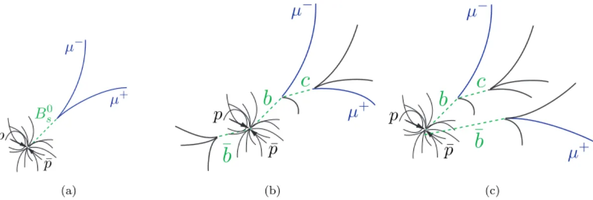
s mass are dominated by double semileptonic decays such as b(¯c) → µ−_{νX and} ¯b(c) → µ+_{νX, as shown in Fig. 2(c). For both of these} backgrounds, the muons do not form a real vertex, but the tracks can occasionally be close enough in space to be reconstructed as a “fake” vertex.

Figure 2 illustrates the differences between signal and background that we exploit as a general analysis strat-egy. The dimuon system itself should form a good vertex consistent with the decay of a single particle originating from the p¯p interaction vertex. The B0

s candidate should have a small impact parameter with respect to the pri-mary p¯p interaction vertex, while the individual muons should in general have fairly large impact parameters. In addition to quantities related to the dimuon system, Fig. 2 illustrates that the environment surrounding the B0

s candidate should be quite different for signal com-pared to backgrounds. The dimuon system for the sig-nal should be fairly well isolated, while the fake dimuon vertex in background events is likely to have additional tracks and additional vertices nearby. No single variable is able to provide definitive discrimination against these backgrounds, so we use a multivariate technique as de-scribed in Sec. VII to exploit these differences between signal and background.

In addition to dimuon backgrounds from semileptonic heavy quark decays, there are peaking backgrounds aris-ing from B0

s→ hh or Bd0→ hh where hh can be KK, Kπ or ππ. Of these, B0

s → KK is the dominant contribution. The K or π mesons can be misidentified as a muon by decay in flight K/π → µν or by penetrating far enough in the detector to create hits in the muon system. For these decays to be misidentified as signal, both hadrons must be misidentified as a muon, but since the decay we are looking for is rare, B0

s/Bd0→ hh decays constitute a background of magnitude similar to that of the expected signal.

The number of B0s → µ+µ −

decays expected in our dataset is determined from analysis of the normalization decay channel B±

→ J/ψK±

, with J/ψ → µ+_µ− , as described in detail in Sec. VI.

(5)

(a) (b) (c)

FIG. 2: (color online) Schematic diagrams showing (a) the signal decay, B0

s → µ +

µ−

, and main backgrounds: (b) sequential

decay, b → cµ−

followed by c → µ+

, and (c) double semileptonic decay, b → µ−

and ¯b → µ+_.

IV. MONTE CARLO SIMULATION

Detailed Monte Carlo (MC) simulations for both the B0

s → µ+µ −

signal and the B±

→ J/ψK±

normalization channels are obtained using the pythia [20] event gen-erator, interfaced with the evtgen [21] decay package. The MC includes primary production of b¯b quarks that are approximately back-to-back in azimuthal angle, and also includes gluon splitting g → b¯b where the gluon may have radiated from any quark in the event. The latter leads to a relatively collimated b¯b system that produces the dominant background when both b and ¯b quarks de-cay semileptonically to muons.

The detector response is simulated using geant [22] and overlaid with events from randomly collected p¯p bunch crossings to simulate multiple p¯p interactions. A correction to the MC width of the dimuon mass distri-bution is determined from J/ψ → µ+µ−

decays in data, and this correction is then scaled to the B0

s mass re-gion. The B0

s → µ+µ −

mass distribution in the MC is well described by a double Gaussian function with the two means constrained to be equal, but with the widths (σ1 and σ2) and relative fractions determined by a fit to the corrected mass distribution. The average width is σav = f σ1+ (1 − f)σ2=125 MeV, where f is the fraction of the area associated with σ1.

We measure the trigger efficiencies in the data using events with no requirements other than a p¯p bunch cross-ing (zero-bias events) or events requircross-ing only an inelastic p¯p interaction (minimum-bias events). The MC gener-ation does not include trigger efficiencies, but the MC events are reweighted to reproduce the trigger efficiency as a function of the muon transverse momentum (pT). In addition, the MC events are corrected to describe the pT distribution of B mesons above the trigger threshold, as determined from B±

→ J/ψK±_{decays. Since the trigger} conditions changed throughout the course of Run II, the pT corrections are determined separately for five different data epochs, with each epoch typically separated by an accelerator shut-down of a few months’ duration.

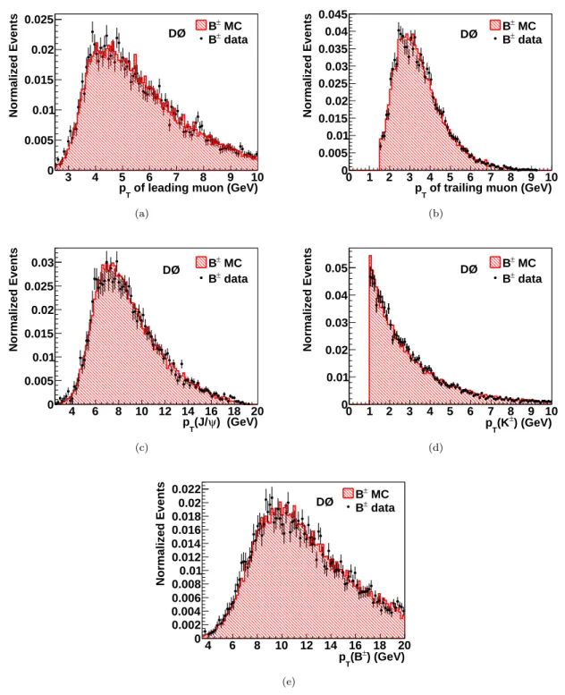
Fig-ure 3 compares data and MC for several pT distributions in the normalization channel, after these corrections. The background components in the B±

distributions are re-moved by a side-band subtraction technique, that is, by subtracting the corresponding distributions from events above and below the B± _{mass region. As can be seen in} Fig. 3, the pTdistributions in the MC simulation and nor-malization channel data are generally in excellent agree-ment. Figure 3 shows a single data epoch, but all data epochs show similar agreement.

In addition to the signal MC, we also study the B0 s→ KK background using a sample of MC events that con-tains about six times the expected number of such events in our data sample.

V. EVENT SELECTION

The B0

s candidate events selected for further study are chosen as follows. We select two high-quality, oppositely-charged muons based on information from both the cen-tral tracker and the muon detectors. The primary vertex (PV) of each p¯p interaction is defined using all available well-reconstructed tracks and constrained by the mean beam-spot position in the transverse plane. If a bunch crossing has more than one p¯p interaction vertex, we en-sure that both muons are consistent with originating from the same PV. Tracks reconstructed in the central tracker are required to have at least two hits in both the SMT and CFT detectors. These tracks are extrapolated to the muon system, where they are required to match hits ob-served in the muon detectors. Each muon is required to have transverse momentum pT > 1.5 GeV and to have pseudorapidity |η| < 2. Both muons are required to have hits in the muon detectors in front of the toroids, and at least one of the muons must also have hits in at least one of the muon layers beyond the toroids. To reduce combinatorial backgrounds, the two muons must form a three-dimensional vertex with χ2_{/dof < 14. The dimuon} vertex is required to be well separated from the PV by

(6)

of leading muon (GeV) T p 3 4 5 6 7 8 9 10 Normalized Events 0 0.005 0.01 0.015 0.02 0.025 MC ± B data ± B DØ (a)

of trailing muon (GeV)

T p 0 1 2 3 4 5 6 7 8 9 10 Normalized Events 0 0.005 0.01 0.015 0.02 0.025 0.03 0.035 0.04 0.045 MC ± B data ± B DØ (b) ) (GeV) ψ (J/ T p 4 6 8 10 12 14 16 18 20 Normalized Events 0 0.005 0.01 0.015 0.02 0.025 0.03 B± MC data ± B DØ (c) ) (GeV) ± (K T p 0 1 2 3 4 5 6 7 8 9 10 Normalized Events 0 0.01 0.02 0.03 0.04 0.05 B± MC data ± B DØ (d) ) (GeV) ± (B T p 4 6 8 10 12 14 16 18 20 Normalized Events 0 0.002 0.004 0.006 0.008 0.01 0.012 0.014 0.016 0.018 0.02 0.022 _B±_MC data ± B DØ (e)

FIG. 3: (color online) Comparison of pTdistributions for data and MC simulation, for the normalization channel B

±

→ J/ψK±,

in a single data epoch, (a) for the higher-pT(leading) muon, (b) lower-pT(trailing) muon, (c) J/ψ, (d) kaon, and (e) B

± meson. All distributions are normalized to unit area.

examining the transverse decay length. The transverse decay length LT is defined as LT = ~lT · ~pT/|~pT|, where the vector ~lT is from the PV to the dimuon vertex in the transverse plane, and ~pT is the transverse momentum vector of the dimuon system. The quantity σLT is the

un-certainty on the transverse decay length determined from

track parameter uncertainties and the uncertainty in the position of the PV. To reduce prompt backgrounds, the transverse decay length significance of the dimuon ver-tex, LT/σLT, must be greater than three. Events are

selected for further study if the dimuon mass Mµµ is be-tween 4.0 GeV and 7.0 GeV. These criteria are intended

(7)

to be fairly loose to maintain high signal efficiency, with further discrimination provided by the multivariate tech-nique discussed in Sec. VII.

The normalization channel decays B±

→ J/ψK± with J/ψ → µ+_µ− _{are reconstructed in the data by first} find-ing the decay J/ψ → µ+_µ− _{and then adding a third} track, assumed to be a charged kaon, to the dimuon ver-tex. The selection criteria for the signal and normaliza-tion channel are kept as similar as possible. In addinormaliza-tion to the above requirements on the muons, we require the K±

to have pT > 1 GeV and |η| < 2, and we require the three-track vertex to have χ2_{/dof < 6.7. In the} normal-ization channel the dimuon mass is required to be in the J/ψ mass region, 2.7 GeV < M (µ+_µ−

) < 3.45 GeV.

VI. DETERMINATION OF THE SINGLE

EVENT SENSITIVITY

To determine the number of B0

s → µ+µ −

decays we expect in the data, we normalize to the number of B±

→ J/ψK±

candidates observed in the data. The number of B±

→ J/ψK±_{decays is used to determine the} single event sensitivity (SES), defined as the branching fraction for which one event is expected to be present in the dataset. The SES is calculated from

SES = _N(B1±₎× ǫ(B±) ǫ(B0 s) f(b→B±) f(b→B0 s)× B(B± → J/ψK± )×B(J/ψ → µ+_µ−_). In this expression N (B± ) is the number of B± → J/ψK± decays observed in the data, as discussed below. The efficiency for reconstructing the normalization channel decay, ǫ(B±_{), and the signal channel, ǫ(B}0

s), are deter-mined from MC simulations as discussed in more detail below. The fragmentation ratio f (b → B±

)/f (b → B0 s) is the relative probability of a b quark fragmenting to a B±

compared to a B0

s. We use the “high energy” average f (b → B0

s)/f (b → B ±

) = 0.263 ± 0.017 provided by the Heavy Flavor Averaging Group [23] for the 2012 Particle Data Group compilation [19], which is consistent with other recent measurements [24]. The product of the branching fractions B(B±

→ J/ψK±

)×B(J/ψ → µ+_µ− ) is (6.01 ± 0.21) × 10−5_[19].

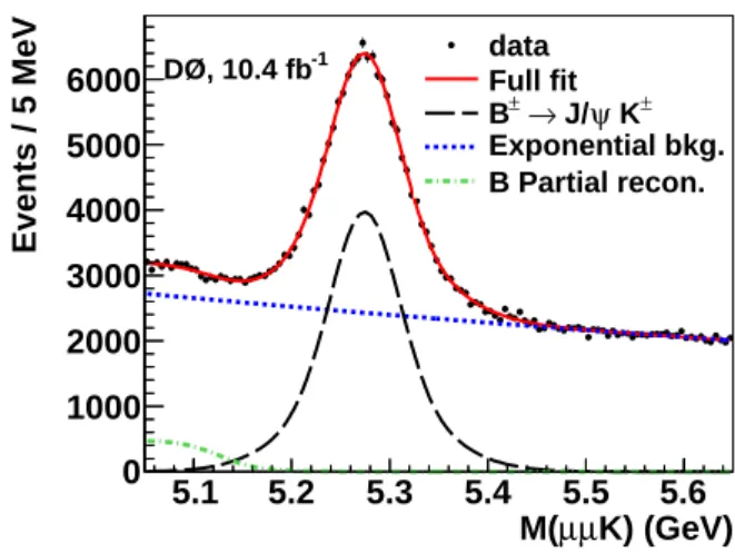
Figure 4 shows the normalization channel mass distri-bution, M (µ+_µ−

K), for the entire Run II dataset. The mass distribution is fitted to a double Gaussian function to model the normalization channel decay and an ex-ponential function to model the dominant background. A hyperbolic tangent threshold function is also included in the fit to model partially reconstructed B meson de-cays, primarily B0

d → J/ψK0∗. A possible contribution from B±

→ J/ψπ± _{is also included in the fit, although} this contribution is not statistically significant and is not shown in the Fig. 4. Systematic uncertainties on N (B±

) are determined from variations in the mass range of the fit, the histogram binning, and the background model. An additional systematic uncertaintity on N (B±_{) is due}

K) (GeV) µ µ M( 5.1 5.2 5.3 5.4 5.5 5.6 Events / 5 MeV 0 1000 2000 3000 4000 5000 6000 data Full fit ± K ψ J/ → ± B Exponential bkg. B Partial recon. -1 DØ, 10.4 fb

FIG. 4: (color online) Invariant mass distribution for the

normalization channel B±

→ J/ψK± for the entire Run

II dataset. The full fit is shown as the solid line, the

B±

→ J/ψK±contribution is shown as the dashed line, the

exponential background is shown as the dotted line, and the contribution from partially reconstructed B meson decays is shown as the dot-dash line.

to the candidate selection. If an event has more than one B±

→ J/ψK± _{candidate, we retain only the} candi-date with the best vertex χ2_{. This choice results in fewer} overall reconstructed B±

→ J/ψK±

decays but also less background. To determine the systematic effect due to this choice, we have reconstructed B±

→ J/ψK± decays in two of the five data epochs retaining all candidates. The SES depends on the ratio N (B±

)/ǫ(B±

), and we find that this ratio varies at most 2.2%, which we take as an additional systematic uncertainty on N (B±

). We observe a total of (87.4±3.0)×103_B±

→ J/ψK± decays in the full dataset, where the uncertainty includes both statistical and systematic effects.

The ratio of reconstruction efficiencies that enters into the SES is determined from MC simulation. One source of systematic uncertainty in the efficiency ratio arises from the trigger efficiency corrections applied to the MC, as described in Sec. IV. The variation in these corrections over data epochs with similar trigger conditions allows us to set a 1.5% systematic uncertainty on the efficiency ratio due to this source. An additional systematic un-certainty arises from the efficiency for finding a third track. There could be a data/MC discrepancy in this efficiency which will not cancel in the ratio. We evaluate this systematic uncertainty by comparing the efficiency for finding an extra track in data and MC in the four-track decay B0

d → J/ψK0∗ with K0∗ → Kπ and in the three-track normalization channel decay B±

→ J/ψK±_. From this study, we determine that the data/MC effi-ciency ratio for identifying the third track varies with data epoch but is on average 0.88 ± 0.06, where the un-certainty includes statistical uncertainties from the fits

(8)

used to extract the number of signal events, and sys-tematic uncertainties estimated from fit variations. The efficiency for B± _{reconstruction is adjusted in each data} epoch for this track-finding efficiency correction. The re-construction efficiency ratio ǫ(B±

)/ǫ(B0

s) is determined to be (13.0 ± 0.5)% on average, but varies over the dif-ferent data epochs by about 1.0%. The efficiency for the B±

→ J/ψK±

decay is impacted by the softer pT dis-tribution of the muons in the three-body decay as well as the fairly hard (pT > 1 GeV) cut on the pT of the kaon, and the candidate selection which retains only the three-track candidate with the best vertex χ2_.

When all statistical and systematic uncertainties are taken into account, the SES is found to be (0.336 ± 0.029) × 10−9 _{before the multivariate selection, yielding} a SM expected number of B0

s → µ+µ −

events of 10.4 ± 1.1 events in our data sample.

VII. MULTIVARIATE DISCRIMINANT

A boosted decision tree (BDT) algorithm, as imple-mented in the tmva package of ROOT [25], is used to differentiate between signal and the dominant back-grounds. The BDT is trained using MC simulation for the signal and data sidebands for the background. The data sidebands include events in the dimuon mass range 4.0–4.9 GeV (low-mass sidebands) and 5.8–7.0 GeV (high-mass sidebands), with all selection cuts applied. The low-mass sidebands are dominated by sequential de-cays, illustrated in Fig. 2(b), while the the high-mass sidebands are dominated by double B hadron decays, as illustrated in Fig. 2(c). We therefore train two BDTs to separately discriminate against these two backgrounds. Each BDT discriminant uses 30 variables that fall into two general classes.

One class of variables includes kinematic and topolog-ical quantities related to the dimuon system. These vari-ables include the pointing angle, defined as the angle be-tween the dimuon momentum vector ~p(µ+_µ−

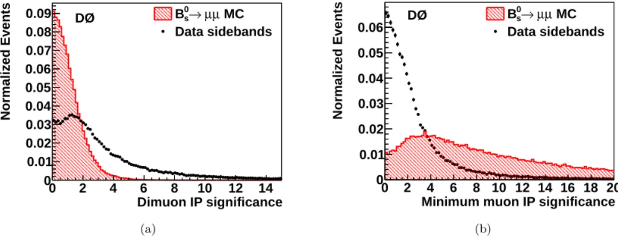
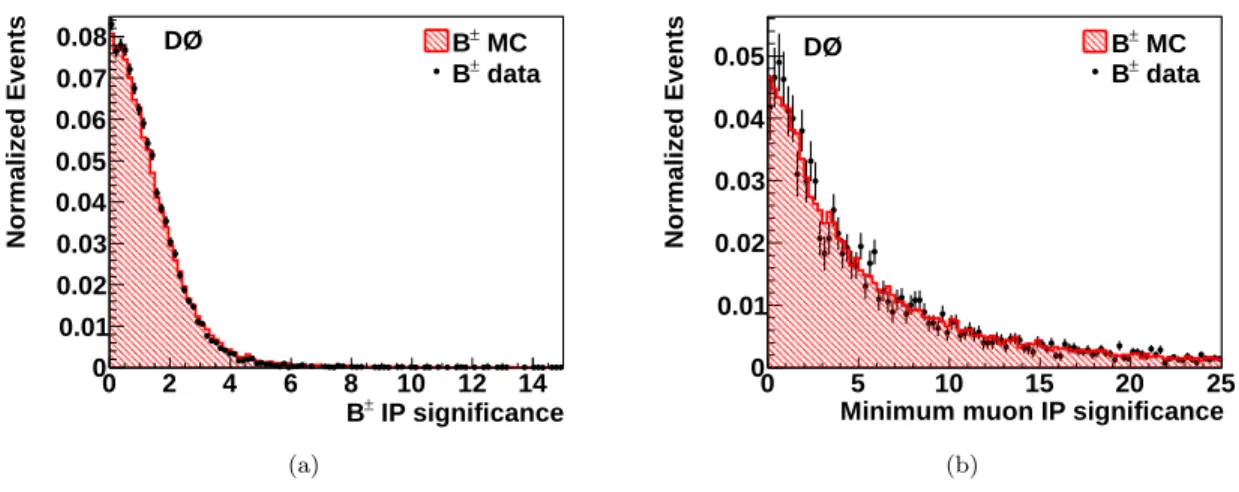
) and the vector from the PV to the dimuon vertex. The dimuon pT and impact parameter, as well as the pT values of the individual muons and their impact parameters, are also used as discriminating variables. As examples of dimuon system variables that discriminate between signal and background, Fig. 5(a) shows the impact parameter sig-nificance (impact parameter divided by its uncertainty) of the B0

s candidate for signal MC and background, and Fig. 5(b) shows the minimum impact parameter signif-icance for the individual muons, that is, the smaller of the two values.

A second general class of variables used in the BDT dis-criminants includes various isolation-related quantities. Isolation is defined with respect to a momentum vector ~p by constructing a cone in azimuthal angle φ and pseudo-rapidity η around the momentum vector, with the cone radius defined by R =p∆η2_{+ ∆φ}2_{. The isolation I is} then defined as I = pT/[pT + pT(cone]) where pT(cone)

is the scalar sum of the pT of all tracks (excluding the track of interest) with R less than some cut-off value, chosen to be R = 1 in this analysis. For a perfectly iso-lated track (that is, no other tracks in the cone), I = 1. Figure 2 shows that background events are expected to be less isolated than signal events. For maximum sig-nal/background discrimination, we define isolation cones around the dimuon direction and around each muon indi-vidually. From simulation studies, we find that for back-ground events, the two muons are often fairly well sepa-rated in space, so using individual isolation cones around each muon adds discriminating power. Figure 6 com-pares signal MC and data sidebands for two examples of isolation variables.

We also search for additional vertices near the dimuon vertex using two different techniques. As illustrated by Fig. 2, in background events the muons often form a good vertex with another charged track. We try to reconstruct such vertices using tracks that are associated with the same PV as the dimuon pair, which have an impact pa-rameter with respect to the PV of at least 30 microns, and which have an impact parameter significance of at least 3.0. If a track satisfying these requirements forms a vertex with one of the muons with a vertex χ2_{/dof < 5.0,} we consider this an additional vertex. Additional tracks, satisfying the same requirements as above, can be in-cluded in this vertex if they do not increase the vertex χ2_{by more than 5.0. This procedure is carried out with} both muons, allowing for the possibility of finding an ad-ditional vertex with either or both of the muons. We also attempt to reconstruct additional vertices using tracks that have an impact parameter significance with respect to the dimuon vertex of less than 4.0. We allow these ver-tices to include or not include one of the muons. When an additional vertex is successfully reconstructed, the vertex χ2, the invariant mass of the particles included in the ver-tex, and the vertex pointing angle are used as discrimi-nating variables in the BDTs. In the case where no such vertices are found, these variables are set to nonphysical values. We find that, for the background sidebands, at least one additional vertex is reconstructed 80% of the time, while for the signal MC, one or more additional vertices are found 40% of the time.

To verify that the MC simulation is a good represen-tation of the data, we compare the sideband-subtracted normalization channel data with the normalization chan-nel MC. Figure 7 compares the normalization chanchan-nel data and the MC simulation for the B±

meson impact parameter significance and the minimum muon impact parameter significance. Figure 8 shows the same com-parison for the dimuon and individual muon isolation variables. We check all 30 variables used in the multi-variate discriminant to confirm good agreement between data and MC for the normalization channel.

We make additional requirements on both the data sidebands and the signal MC before events are used in the BDT training. These requirements include dimuon pT > 5 GeV and the cosine of the dimuon pointing angle

(9)

Dimuon IP significance 0 2 4 6 8 10 12 14 Normalized Events 0 0.01 0.02 0.03 0.04 0.05 0.06 0.07 0.08 0.09 B0s→µµ MC Data sidebands DØ (a)

Minimum muon IP significance 0 2 4 6 8 10 12 14 16 18 20 Normalized Events 0 0.01 0.02 0.03 0.04 0.05 0.06 MC µ µ → 0 s B Data sidebands DØ (b)

FIG. 5: (color online) Comparison of signal MC and background sideband data for (a) the B0

s candidate impact parameter

significance and (b) the minimum muon impact parameter significance. All distributions are normalized to unit area.

Dimuon isolation 0 0.2 0.4 0.6 0.8 1 Normalized Events 0 0.02 0.04 0.06 0.08 0.1 0.12 0.14 0.16 0.18 B0s→µµ MC Data sidebands DØ (a)

Individual muon isolation

0 0.2 0.4 0.6 0.8 1 Normalized Events 0 0.01 0.02 0.03 0.04 0.05 0.06 0.07 0.08 0→µµ MC s B Data sidebands DØ (b)

FIG. 6: (color online) Comparison of signal MC and background sideband data for (a) isolation defined with respect to the dimuon system and (b) for the average of the two isolations defined with respect to the individual muons. All distributions are normalized to unit area.

> 0.95. These requirements are 78% efficient on average in retaining signal events but exclude about 96% of the background. We find a significant enhancement in back-ground rejection from the BDT discriminants using these additional requirements before BDT training. These re-quirements are (93 ± 1)% efficient for the normalization mode MC, and (91 ± 3) % efficient for the normalization mode data.

To improve the statistics available for training, the data epochs are combined and used together to train the BDT. The signal MC samples for each data epoch are combined according to the integrated luminosity for each epoch into a common sample. The data sidebands and signal MC are then randomly split into three samples. Sample A, with 25% of the events, is used to train the BDTs. Sample B, with 25% of the events, is used to opti-mize the selections on the BDT response. Sample C, with

50% of the events, is used to determine the expected sig-nal (from the MC sample) and background (from the data sideband sample) yields. The results of the TMVA BDT training for both BDT1, trained to remove sequential de-cay backgrounds, and BDT2, trained to remove double semileptonic B meson decays, can be seen in Fig. 9. We check that the response of both BDT discriminants is in-dependent of dimuon mass over the relevant mass range. The optimal BDT selections are determined by optimiz-ing the expected limit on B(B0

s→ µ+µ −

) and are found to be BDT1 > 0.19 and BDT2 > 0.26.

(10)

IP significance ± B 0 2 4 6 8 10 12 14 Normalized Events 0 0.01 0.02 0.03 0.04 0.05 0.06 0.07 0.08 B± MC data ± B DØ (a)

Minimum muon IP significance

0 5 10 15 20 25 Normalized Events 0 0.01 0.02 0.03 0.04 0.05 B± MC data ± B DØ (b)

FIG. 7: (color online) Comparison of normalization channel MC and sideband-subtracted data for (a) B±

impact parameter significance and (b) the minimum muon impact parameter significance. All distributions are normalized to unit area.

Dimuon isolation 0 0.2 0.4 0.6 0.8 1 Normalized Events 0 0.02 0.04 0.06 0.08 0.1 0.12 0.14 B± MC data ± B DØ (a)

Individual muon isolation

0 0.2 0.4 0.6 0.8 1 Normalized Events 0 0.01 0.02 0.03 0.04 0.05 0.06 0.07 0.08 0.09 0.1 MC ± B data ± B DØ (b)

FIG. 8: (color online) Comparison of normalization channel MC and sideband-subtracted data for (a) dimuon isolation and (b) the average of the two individual muon isolations. All distributions are normalized to unit area.

VIII. BACKGROUND ESTIMATES AND

EXPECTED LIMIT

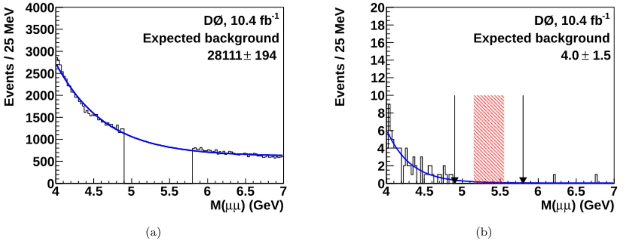
Figure 10 shows the blinded dimuon mass distribu-tions before (Fig. 10(a)) and after (Fig. 10(b)) the BDT selection cuts for the half of the data (sample C) used to estimate the number of background events. The sig-nal window within the blinded region is chosen to maxi-mize the signal significance S/√S + B, where S is the expected number of signal events as determined from the SM branching fraction, and B is the expected back-ground. The number of expected background events is determined by a likelihood fit to the data in the side-band regions, which is then interpolated into the blinded region. The optimum signal region is determined to be ±1.6σ centered on the B0

s mass, where σ = 125 MeV is the average width of the double Gaussian used to fit

the dimuon mass distribution in the B0

s → µ+µ −

MC sample. The blinded region includes a control region of width 2σ on each side of the signal window. While only half of the dataset is shown, the numbers of expected background events quoted in Fig. 10 are scaled to the full dataset. The numbers given are for the estimated dimuon background events in the signal region.

The efficiency for retaining signal events when all BDT selections are applied, including the pre-training cuts (see Sec. VII) and the final BDT cuts, is determined to be 0.12 ± 0.01, where the error is due to variation over the different data epochs. We obtain a final SES of (2.8 ± 0.24)×10−9_{, corresponding to an expected number} of signal events at the SM branching fraction of 1.23 ± 0.13. For the dimuon background the expected number of events in the signal and control regions is determined by applying a log likelihood fit to the dimuon mass

(11)

dis-BDT1 response -0.6 -0.4 -0.2 0 0.2 0.4 0.6 Normalized Events 0 0.01 0.02 0.03 0.04 0.05 0.06 0_→_µ_µ_MC s B Data sidebands DØ (a) BDT2 response -0.6 -0.4 -0.2 0 0.2 0.4 0.6 Normalized Events 0 0.01 0.02 0.03 0.04 0.05 →µµ MC 0 s B Data sidebands DØ (b)

FIG. 9: (color online) Distributions of the BDT response for (a) BDT1, trained against sequential decay backgrounds, and (b) BDT2, trained against double B decay backgrounds. MC simulation is used for the signal, while the data sidebands are used for the backgrounds. The vertical lines denote the BDT selection cuts in the analysis. All distributions are normalized to unit area. ) (GeV) µ µ M( 4 4.5 5 5.5 6 6.5 7 Events / 25 MeV 0 500 1000 1500 2000 2500 3000 3500 4000 -1 DØ, 10.4 fb Expected background 194 ± 28111 (a) ) (GeV) µ µ M( 4 4.5 5 5.5 6 6.5 7 Events / 25 MeV 0 2 4 6 8 10 12 14 16 18 20 Expected background 1.5 ± 4.0 -1 DØ, 10.4 fb (b)

FIG. 10: (color online) Dimuon mass distribution for sample C (a) before and (b) after BDT selection cuts. The edges of the blinded region are denoted in (b) by the vertical lines at 4.9 and 5.8 GeV, and the shaded area denotes the signal window. The curves are fits to an exponential plus constant function. The numbers of expected background events are determined from an interpolation of the fit into the signal window and scaled to the full dataset.

tribution using an exponential plus constant functional form. The fit is performed excluding the blinded region, and the resulting fit is interpolated into the signal and control regions. This procedure yields an expected num-ber of dimuon background events in the signal region of 4.0 ± 1.5 events, where the uncertainty is only statisti-cal. The corresponsing estimate for the expected num-ber of events in the control region is 6.7 ± 2.6 events, with 5.3 ± 1.9 events expected in the lower control region (dimuon masses from 4.9 to 5.15 GeV), and 1.4 ± 1.4 events in the upper control region (dimuon masses from 5.55 to 5.8 GeV). To determine the systematic uncer-tainty on the background estimate, we use other func-tional forms for the background fit, resulting in a

sys-tematic uncertainty of 0.6 events. Adding the statistical and systematic errors in quadrature yields a final dimuon background estimate in the signal region of 4.0 ± 1.6 events and 6.7 ± 2.7 events in the control region.

In addition to the dimuon background, there is back-ground from the decay mode B0

s → K+K −

, which has kinematics very similar to the signal. We estimate this background by scaling the expected number of signal events by the appropriate branching fractions [19] and by the ratio of the probabilities for both K mesons to be misidentified as muons, ǫ(KK → µµ), to the proba-bility that two muons are correctly identified as muons, ǫ(µµ → µµ). The probability that a K meson is misiden-tified as a muon is measured in the data using D0_{→ Kπ}

(12)

decays. We assume that the probability of two K mesons being misidentified as muons is the product of the proba-bilities for each individual K meson. The muon identifi-cation efficiency is measured in the data from J/ψ → µµ decays. The efficiency ratio ǫ(KK → µµ)/ǫ(µµ → µµ) is determined to be (3.0 ± 1.1) × 10−5_{. We estimate the} background from B0

s → KK decays to be 0.28 ± 0.11 events. We also find a consistent estimate of this back-ground using a B0

s → KK MC sample. Other possible peaking backgrounds such as B0

d → Kπ and B 0 s → Kπ are negligible due to the combination of smaller branch-ing fractions and a π → µ misidentification probability that is more than a factor of 10 smaller than the K → µ misidentification probability in the D0 detector.

We set an upper limit on the B0

s → µ+µ

− _branching fraction using the CLs, or modified frequentist method [26]. A Poisson likelihood function is used to calculate the number of signal events which would occur with a probability of 0.05 (for a 95% CL upper confidence limit) when Nobs data events are observed in the signal region with a known expected number of background events.

The limit calculation includes a convolution over prob-ability distributions representing the uncertainties in the background and the signal. The uncertainty in the B0

s → KK peaking background is assumed to be Gaus-sian. The dimuon background in the signal region is es-timated by the fit shown in Fig. 10(b). The normalized likelihood function from this fit is used as the probability distribution function for the dimuon background in the convolution. The expected number of signal events, as-suming the SM branching fraction, is 1.23 ± 0.13 events, with the uncertainty assumed to be Gaussian. The total expected background is 4.3 ± 1.6 events. Weighting each possible outcome by its Poisson probability yields an ex-pected 95% C.L. upper limit on the branching fraction B(B0

s→ µ+µ −

) of 23 × 10−9_.

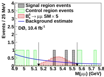
Upon unblinding, a total of nine events is found in the control region above and below the signal region, as shown in Fig. 11. Six events are found in the control re-gion below the signal window, and three events are found in the control region above the signal window. This num-ber of events and their distribution within the control re-gions is in agreement with the expected number of back-ground events interpolated from the data sidebands. As seen in Fig. 11, three events are found in the dimuon mass signal window, in agreement with the expected back-ground and also with the expected signal + backback-ground. We check that the properties of all events found in the blinded region, such as the pT of the dimuon system, the pT of the individual muons, the dimuon pointing angle, and the various isolation quantities, are consistent with expectations. We also check that, as the BDT cuts are re-laxed, the number of events observed in the signal region remains in good agreement with expectations, as shown in Fig. 12.

The observed number of events and the SES allow us to set a 95% C.L. upper limit B(B0

s→ µ+µ − ) < 15 × 10−9_. ) (GeV) µ µ M( 4.9 5 5.1 5.2 5.3 5.4 5.5 5.6 5.7 5.8 Events / 25 MeV 0 0.5 1 1.5 2 2.5 3 3.5

4 _{Signal region events}

Control region events 5 × SM µ µ → 0 s B Background estimate -1 DØ, 10.4 fb

FIG. 11: (color online) Dimuon mass distribution in the blinded region for the full dataset after BDT selections are applied. The curve shows the fit from Fig. 10(b) used to de-termine the expected number of background events. The SM expectation for signal events multiplied by five is also indi-cated. The vertical lines mark the edge of the signal window.

BDT2 0.21 0.22 0.23 0.24 0.25 0.26 Events 0 2 4 6 8 10 12 14 16 18 Expected events Observed events BDT1 0.15 0.16 0.17 0.18 0.19

FIG. 12: (color online) Expected number of events and ob-served number of events in the signal region as the two BDT cuts are relaxed in parallel. The expected number of events

includes the dimuon background, the B0

s→ KK background,

and the expected number of signal events. The upper hori-zontal axis shows the cut applied to BDT1, while the lower horizontal axis shows the cut applied to BDT2.

IX. SUMMARY

In summary, we have searched for the rare decay Bs0 → µ+µ

−

in the full D0 dataset. We employ two Boosted Decision Tree multivariate discriminators, one trained to discriminate against sequential decays b(¯b) → cµ−_(¯_cµ+_{)X followed by c(¯}_{c) → µ}+_(µ−_{)X and the other}

(13)

to discriminate against double semileptonic decays b → µ−

X and ¯b → µ+_{X. The sidebands around the signal} re-gion in the dimuon invariant mass distribution are used to estimate the dominant backgrounds. The expected limit is 23 ×10−9_{, and the expected background (signal)} in the signal region is 4.3 ± 1.6 (1.23 ± 0.13) events. We observe three events in the signal region consistent with expected background. The probability that the back-ground alone (signal + backback-ground) could produce the observed number of events or a larger number of events in the signal region is 0.77 (0.88). We set an observed 95% C.L. upper limit B(B0

s→ µ+µ −

) < 15 × 10−9_{. This} upper limit supersedes the previous D0 95% C.L. limit of 51 ×10−9 _{[10], and improves upon that limit by a} fac-tor of 3.4. The improvement in the expected limit is a factor of 1.7 greater than the improvement that would be expected due to increased luminosity alone. The ad-ditional improvement arises from the inclusion of several

isolation-type variables in the multivariate discriminants and in the use of two separate discriminants to distin-guish backgrounds from sequential b quark decays and double b quark decays. This result is the most stringent Tevatron limit and is compatible with the recent evidence of this decay produced by the LHCb experiment [11].

We thank the staffs at Fermilab and collaborating in-stitutions, and acknowledge support from the DOE and NSF (USA); CEA and CNRS/IN2P3 (France); MON, NRC KI and RFBR (Russia); CNPq, FAPERJ, FAPESP and FUNDUNESP (Brazil); DAE and DST (India); Col-ciencias (Colombia); CONACyT (Mexico); NRF (Ko-rea); FOM (The Netherlands); STFC and the Royal So-ciety (United Kingdom); MSMT and GACR (Czech Re-public); BMBF and DFG (Germany); SFI (Ireland); The Swedish Research Council (Sweden); and CAS and CNSF (China).

[1] K. De Bruyn et al., Phys. Rev. Lett. 109, 041801 (2012). [2] A. J. Buras et al., Eur. Phys. J. C72, 2172 (2012). [3] A. J. Buras, Acta. Phys. Polon. B 41, 2487 (2010). [4] S. R. Choudhury and N. Gaur, Phys. Lett. B 451, 86

(1999).

[5] J. K. Parry, Nucl. Phys. B760, 38 (2007).

[6] R. L. Arnowitt, B. Dutta, T. Kamon and M. Tanaka, Phys. Lett. B 538, 121 (2002).

[7] J. R. Ellis, J. S. Lee, and A. Pilaftsis, Phys. Rev. D 76, 115011 (2007).

[8] V. Abazov et al. (D0 Collaboration), Phys. Rev. Lett.

94, 071802 (2005).

[9] V. Abazov et al. (D0 Collaboration), Phys. Rev. D 76, 092001 (2007).

[10] V. M. Abazov et al. (D0 Collaboration), Phys. Lett. B

693_{, 534 (2010).}

[11] R. Aaij et al. (LHCb Collaboration), Phys. Rev. Lett.

110, 021801 (2013).

108, 231801 (2012).