HAL Id: hal-01096602
https://hal.inria.fr/hal-01096602
Submitted on 7 Jan 2015
HAL is a multi-disciplinary open access
archive for the deposit and dissemination of
sci-entific research documents, whether they are
pub-lished or not. The documents may come from
teaching and research institutions in France or
abroad, or from public or private research centers.
L’archive ouverte pluridisciplinaire HAL, est
destinée au dépôt et à la diffusion de documents
scientifiques de niveau recherche, publiés ou non,
émanant des établissements d’enseignement et de
recherche français ou étrangers, des laboratoires
publics ou privés.
Natural Information Flow Propagation to Simulate
Growing Dynamical Systems
Jean-Philippe Bernard, Benjamin Gilles, Christophe Godin
To cite this version:
Jean-Philippe Bernard, Benjamin Gilles, Christophe Godin.
Combining Finite Element Method
and L-Systems Using Natural Information Flow Propagation to Simulate Growing Dynamical
Sys-tems. TPNC: Theory and Practice of Natural Computing, Dec 2014, Granada, Spain. pp.218-230,
�10.1007/978-3-319-13749-0_19�. �hal-01096602�
L-Systems Using Natural Information Flow
Propagation to Simulate Growing Dynamical
Systems
Jean-Philippe Bernard1, Benjamin Gilles2, and Christophe Godin1
1 Inria, Virtual Plants project-team, Universit´e Montpellier 2, Bˆatiment 5, CC 06002, 860 rue de Saint Priest, 34095 Montpellier Cedex 5, France 2 CNRS, Laboratoire d’Informatique, de Robotique et de Micro´electronique de Montpellier, Universit´e Montpellier 2, Bˆatiment 5, CC 06002, 860 rue de Saint Priest,
34095 Montpellier Cedex 5, France
Abstract. This paper shows how to solve a system of di↵erential equa-tions controlling the development of a dynamical system based on finite element method and L-Systems. Our methods leads to solve a linear system of equations by propagating the flow of information throughout the structure of the developing system in a natural way. The method is illustrated on the growth of a branching system whose axes bend under their own weight.
1
Introduction
Plants are complex branching organisms that undergo continuous development throughout their lifetime. To understand the key processes that control this development, a new type of modeling approach, called Functional-Structural Plant Models (FSPM) [8, 19, 17], has been developed in the last two decades. FSPMs combine a detailed description the plant architecture (in terms of axes or stem units) and physiological processes that participate to the branching system development (photosynthesis, water/sugar/mineral element transport, carbon allocation, bud growth, hormonal transport and regulation, interaction with gravity, etc.).
To build FSPMs, L-systems [16] have emerged as a dominant paradigm to describe both the development plant branching systems in time and to model the di↵erent bio-physical processes of interest [14, 3]. L-systems make it possible to model the development of a plant by specifying rules of development for the di↵erent types of considered plant constituent in a declarative manner. At each time step, the language engine scans the constituents of the branching structure being computed and applies the developmental rule that corresponds to its type. Interestingly, at no moment the modeler needs to index the plant elements. As the rules are supposed to be local, it is sufficient in the rule specification to access the immediate neighbor components, for example referring in the rule to the predecessor and successor components of the current plant component.
The propagation of a signal from the basis of the plant to the top provides a good example of such a principle of locality. Let a plant be represented a bracketed string I I [ I I ] I [ I ] I. This string represents a branching structure containing 6 components, all of type I (note that the structure contains no indexing of the components). Two consecutive I’s represent two consecutive segments in the same axis of the plant, while a bracket indicates a branch inserted at the top of preceding left-hand component (Fig. 1). Then, let us imagine that the leftmost component in the string (at the plant basis) contains a signal x = 1, and that the signal x is set to 0 in all the other components. To propagate the signal in time through the plant body, one needs to define a simple local rule such as (in pseudo-code form):
I --> { if p r e d e c e s s o r() .x == 1 then current() .x = 1 } produce I
meaning that a I symbol should be transformed over one time step in a I symbol (produce statement) after having set its internal signal value x to 1 if the x signal of the predecessor components in the plant was itself at set at 1. This
I I I I I I I I I I I I I I I I I I I I I I I I I I I I
Fig. 1. Branch represented L-string I I [ I I ] I [ I ] I with information x = 1 (red segments) propagation to others segments (blue).
local rule makes it possible to get completely rid of indexes when transferring information through the plant structure [13]. This specific feature of L-systems was used in the last decade to develop computational models for which the flow of information propagates in a natural way over the plant structure from component to component, e.g. [1] for the transport of carbon, [15] for the transport of water, and [10, 5] for the reaction of plants to gravity. All these algorithms use finite di↵erence methods (FDM) for which the plant is decomposed into a finite number of elements and quantities of interest (water content, sugar concentration, forces, displacements, etc.) correspond to discrete values attached to each component. Di↵erent FDM schemes have been developed for this based either on explicit or implicit methods [7, 9].
FDM approaches use a local Taylor expansion to approximate di↵erential equations and are easy to implement. However, the quality of the approximation between grid points is generally considered poor. The Finite Element Method is an alternative solution that uses an integral formulation. While more com-plex to implement, the quality of a FEM approximation is often higher than in the corresponding FDM approach [11]. In this paper, we intend to adapt the
FEM approach to be used in the context of L-systems and natural computing, i.e. strictly respecting the paradigm of computational locality, and solving the di↵erential equation by propagating information flows throughout the structure being computed. We illustrate and assess our generic approach on the problem of computing the e↵ect of gravity on growing branching systems.
2
Natural Computing of Branch Bending Using Finite
Di↵erence Method (FDM) and L-Systems
2.1 Mechanical Model of Branch Bending
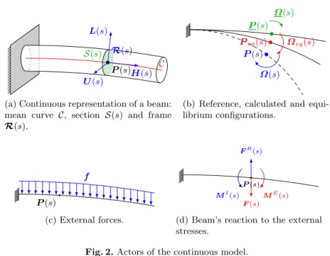
We model a branch as a set of inextensible elastic cantilever beams rigidly con-nected to each other and forming a branching network. Each beam represents a botanical axis and is conceptualized as a mean curveC of length L with natural parameter s2 [0, L] denoting the arc-length distance of a point P (s) from the base of the stem and a sectionS(s) (Fig. 2a).
Each point P (s) is associated with an orthonormal local frame R(s) = {H(s), L(s), U(s)} (heading, left and up) similar to the Frenet’s coordinate system [16]. We assume that vector H(s) is tangent to the rod axis and vectors L(s) and U (s) areC0-continuous with respect to s. Since all vectors H(s) have
unit length the point P (s), s2 [0, L] is defined by: P (s) = P (0) +
Z s 0
H(u) du. (1)
Let P (s) and P (s + ds) be two infinitesimally close points on the curve C. Then the local frame R(s + ds) can be obtained from R(s) by a rotation of axis (s) and angle ✓(s). It is convenient to represent this rotation by a vector ⌦(s), called the generalized curvature, whose direction is the rotation axis (s) and whose norm is ✓(s) (Fig. 2b) [10]. If the arc length ds is infinitesimal, this rotation can be factorized as a rotation around the tangent (twist) and a rotation around the normal (curvature) of the mean curveC at the point P (s). Starting from an initial frame R(0), the frames R(s) can be obtained thanks to the ordinary di↵erential equation (2) [10]:
dsR(s) = [⌦(s)]⇥R(s), (2)
where [⌦(s)]⇥denote respectively the skew-symmetric matrix corresponding to the cross product of ⌦(s) with an other vector (Eq. (3))andR(s) denotes the column matrix⇥H(s), L(s), U (s)⇤. ⌦⇥ v = 2 4⌦⌦01 ⌦2 3 5 ⇥ 2 4vv01 v2 3 5 = 2 4⌦02 ⌦02 ⌦⌦10 ⌦1 ⌦0 0 3 5 2 4vv01 v2 3 5 = [⌦]⇥v (3)
At rest, the branch geometry is characterized by its generalized curvature ⌦ and defines the reference configuration. At each point P (s), the elastic deforma-tion of the material induces internal moments MI(s) (departure from the rest
C P (s) S(s) H(s) L(s) U (s) R(s)
(a) Continuous representation of a beam: mean curve C, section S(s) and frame R(s). Peq(s) ⌦eq(s) P (s) ⌦(s) P (s) ⌦(s)
(b) Reference, calculated and equi-librium configurations. P (s) f (c) External forces. ME(s) F (s) MI(s) FR(s) P (s)
(d) Beam’s reaction to the external stresses.
Fig. 2. Actors of the continuous model.
configuration). We assume here for simplicity a linear constitutive law (Hooke’s law). Classical beam theory [4] allows to compute those moments (Eq. (4)), as a function of the di↵erence between the reference and actual generalized curvatures ⌦ and ⌦:
MI(s) =R(s)C(s)R(s)T(⌦(s) ⌦(s)) =K(s) (⌦(s) ⌦(s)) , (4) whereK(s) is the sti↵ness matrix. Note that the Hooke matrix C(s) expressed in the local frameR(s) is diagonal. Its coefficients are the twist rigidity CH(s) (in
the plane (L(s), U (s)), as a function of sectionS(s) and shear modulus G) and the flexural rigidities CL(s) and CU(s) (respectively in the planes (U (s), H(s))
and (H(s), L(s)), as a function of sectionS(s) and young modulus E):
C(s) = 2 4CH·(s)CL·(s) ·· · · CU(s) 3 5 ; 8 > < > : CH(s) = GRS(s)u2+ v2dS CL(s) = ERS(s)u2dS CU(s) = ERS(s)v2dS , (5)
where (u, v) are the coordinates in the plane (L(s), U (s)), with origin P (s). When external forces f (such as the weight f = ⇢g, Fig. 2c) are applied to the branch, external moments are induced. They result exclusively from the force densities f ([s, L]) present downstream of P (s). Denoting F (s) = RsLf (u) du the external force applied to segment [s, L] due to gravity, we can express the
external moments as a function of forces F and tangents H: ME(s) = Z L s (P (u) P (s))⇥ f(u) du = Z L s
H(u)⇥ F (u) du. (6) At equilibrium, the internal torque (induced by deformation) exactly balances the external torque (induced by external forces) (Fig. 2d):
K(s) (⌦(s) ⌦eq(s)) + ME(s) = 0, (7)
where ⌦eqdenotes the generalized curvature at equilibrium:
⌦eq(s) = ⌦(s) +K(s) 1ME(s). (8)
2.2 FDM Discretization and Natural Integration Using L-Systems Let us discretize the curveC into a set of I + 1 nodes Niof curvilinear abscissa
si, i = 0 . . . I (usually regularly spaced though not necessarily) so that N0 =
P (0) and NI = P (L). Each node is associated with its position Pi, frame
Ri, external moments MEi or accumulated downstream forces Fi. If distances
dsi=ksi+1 sik are small enough, we can express (1), (2), and (6) thanks to
Taylor’s series at order 1 (Euler methods) [12].
Interestingly, point Pi+1 and frame Ri+1 can be recursively expressed in
terms of the previous point Pi and frameRi, which allow us to compute these
quantities in a single pass from the basis of the curve to its tip [18].
Pi+1= Pi+ dsiHi, (9)
Ri+1=Ri+ dsi[⌦i]⇥Ri. (10)
Likewise, external moments MEi 1 and accumulated forces Fi 1 can be
re-cursively expressed in terms of MEi and Fiat the next node. Their computation
can thus be carried out in a single pass from curve tip to basis.
MEi 1= MEi + dsi 1Hi⇥ Fi, (11)
Fi 1= Fi+
Z si
si 1
f (u) du. (12)
Due to large deformations, (7) is non-linear in terms of generalized curvature. To solve it, we use an explicit iterative method, and, specifically, a relaxation method [12] with a factor r2]0, 1[:
⌦t+1(s) = (1 r)⌦t(s) + r(⌦(s) +Kt(s) 1ME t(s)), (13) with ⌦0(s) = ⌦(s). The iterative process stops when the di↵erence between two successive solutions is smaller than a tolerancek⌦t+1 ⌦tk < ".
The above recursive formulation makes it possible to define local L-system rules that will propagate in two pass across the branch structure, from node to node. The flow of computation goes as follows between two time steps:
Input: branch at time t
Output: branch at time t + 1
do:
L - system pass from tip to basis
# c o m p u t a t i o n of (11), (12), (13)
L - system pass from basis to tip
# c o m p u t a t i o n of (9), (10)
until c o n v e r g e n c e c o n d i t i o n of (13) reached
Sketch of a L-system rule used for the tip-to-basis pass
N --> { ds = abs ( s u c c e s s o r() .s - current() .s )
current() .F = s u c c e s s o r() .F + ds * s u c c e s s o r() .f
# ... c o m p u t a t i o n of (11) and (13)
} produce N
Sketch of a L-system rule used for the basis-to-tip pass
N --> { ds = abs ( p r e d e c e s s o r() .s - current() .s )
current() .P = p r e d e c e s s o r() .P + ds * p r e d e c e s s o r.H
# ... c o m p u t a t i o n of (9), (10)
} produce N
3
Natural Computing of Branch Bending Using Finite
Element Method (FEM) and L-Systems
3.1 Computing Axis Bending by Axial Information Propagation with FEM
In FDM and FEM, continuous model domains are approximated using informa-tion at a finite number of discrete locainforma-tions called nodes Ni, i = 0, . . . , I. Whereas
in FDM, solutions are only evaluated at nodes (and not elsewhere within the domain), in FEM the set of nodes correspond to the vertices of polygonal ele-ments that tile the domain of interest. The solution is evaluated at each node using an integral formulation and interpolated over the whole domain using a basis of shape functions 'i associated with each node Ni) [2]. Here, our aim is
to compute the generalized curvature ⌦ that characterizes the axis shape on the whole domain (i.e. on the curveC). For this we decompose ⌦ on the set of shape functions: ⌦(s) = I X i=0 ⌦i'i(s), (14)
where ⌦iis a vector. Shape functions 'iare usually low order polynomials that
are null on all node Nj6= Niand have value 1 at node Ni. They are interpolating
and form a partition of unity [2]. Their support is compact and their values at one node influences those of neighboring elements.
To compute values ⌦ion nodes Ni, we have to solve the linear systemMX = B defined by 15, [2]: I X i=0 ⌦i |{z} =XT i Z C 'i(s)'j(s) ds | {z } =Mji = Z C ⌦(s)'j(s) ds + Z CK(s) 1ME(s)' j(s) ds | {z } =BT j , (15)
whereMijcorrespond to the energy of the cross influence of nodes Njand Nion
the axis, Xi= ⌦Ti and Bito the energy of forces along the axis which influence
the generalized curvature ⌦i of the node Ni. If the mass-matrix coefficientMji
can be analytically computed (shape function are known) and expressed as a sum of integrals on each element, we have to compute numerically the right hand-side Bj. Because this term is not linear, we split up each element in several
integration areas and use midpoint method [12] to numericaly approach the integrals (note that one may also use the Gauss points method [12]).
Properties of mass-matrix (symmetric and positive definite) allow us to use a Cholesky decomposition [12] (product of a low triangular matrix with its trans-pose) to solve in two data propagation through the structure thanks to forward substitution (17) and backward substitution (18) algorithms [12].
M = LLT , 8 > > < > > : Lij= Mij Pj 1 k=0LikLjk Ljj ,80 6 j < i 6 I Lii= q Mii Pi 1k=0L2ik, 80 6 i 6 I (16) LY = B , Yi= Bi Pi 1k=0LikYk Lii ,80 6 i 6 I (17) LTX = Y , X i= Yi PIk=i+1LkiYk Lii ,8I > i > 0 (18) Cholesky decomposition (16) and forward substitution (17) algorithms can be computed together with one pass, e.g. from basis-to-tip (resp. from tip to basis) and the backward substitution (18) algorithm can be computed with an a pass in the reverse direction, e.g. from tip to basis (resp. from basis to tip). 3.2 Extension to Branching Systems
We now need to extend the previous algorithm so that it can cope with branching organizations of beams that would represent plant structures. As in a branch-ing structure, each element has only one parent, ramifications do not influence forward propagations (update of framesR(s) and points P (s)).
Solving the linear system MX = B is more difficult in case of ramification than in the case of a single axis. Non-null elementsMij in the matrixM
corre-spond to branch segments between nodes Ni and Nj such that the product of
the shape functions 'i and 'j along these segments is non-null. Therefore, the
consider two indexing strategies: a forward and a backward strategies indexing respectively the elements from basis to tip (matrix Mf) and from tip to basis
(matrixMb). Using either of indexing strategies, matrices have a block structure
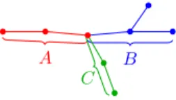
according to the set of nodes between two branching points (Fig. 3).
A B
C
Fig. 3. Sets of nodes corresponding to each block of matricesMf andMb.
Mf = 2 4M f AA sym Mf ABM f BB Mf AC · M f CC 3 5 ; Mb= 2 4M b BB sym · Mb CC Mb AB MbACMbAA 3 5 . (19) With the same notations, we can computeLf andLbthe Cholesky
decompo-sition matrices ofMf =LfLf T andMb=LbLbTrespectively. Then, building the
direted acyclic graphs that correspond to data propagation in Cholesky decom-position algorithm. It is possible to show that only the Cholesky decomdecom-position Lb keeps non-null coefficients at exactly the same places as those of the original
matrixMb (Fig. 4) [6]. Lf AA Lf AB L f BB Lf AC L f BC L f CC Mf AA Mf AB M f BB Mf AC M f BC M f CC = 0 6= 0
(a) Forward indexing.
Lb BB Lb BC LbCC Lb AB LbAC LbAA Mb BB Mb BC MbCC Mb AB MbAC MbAA = 0 = 0 (b) Backward indexing.
Fig. 4. Direted acyclic graphs that correspond to data propagation in Cholesky de-composition algorithm. With a forward indexing,Lf
BC6= 0 whereas M f
BC= 0 contrary to a backward indexing whereLbBC= 0 =MbBC.
3.3 Natural Computing Using L-System
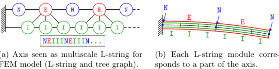
On an axis, elements and integration domains are segments. Since a node has influence only on its neighboring elements (possibly at order greater than 1), we can express our model in L-systems:
– a node is represented by a module of typeN,
– an element between two nodes is represented by a module of typeE, – elementsEare decomposed into integration segments represented by modules
of typeI.
Because two elements can be decomposed into two di↵erent number of inte-gration segments, and a node influences always the same number of neighboring elements, we chose to use a multiscale L-string representation [3] to carry out the integral calculus. Thus the axis is represented at two scales: the scale of nodes and elements and the scale of integration points. The first scale is used to assemble the mass-matrix Mb and solve the linear systemMbX = B whereas
the second scale is used to compute B.
N E N E N
I I I I I I
NEIIINEIIIN...
(a) Axis seen as multiscale L-string for FEM model (L-string and tree graph).
E E I I I I I I N N N
(b) Each L-string module corre-sponds to a part of the axis. Fig. 5. Di↵erent representations of a multiscale L-string.
stored in the node Ni.
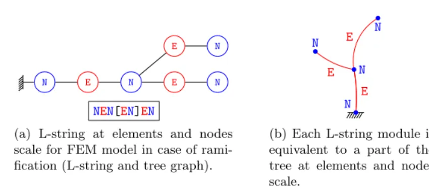
When a ramification exists, we deal with it in L-system by adding brackets after a node N to begin a new axis having this node as a root. The L-string
NEN[EN]EN corresponds to a simple branch composed of a segment axis E di-vided in two axis segments (Fig. 6a and 6b). Like previously, each elementEis decomposed into several integration segmentsIat a lower scale.
Using this data structure and storing each row of matrices from their diagonal to their last coefficient in the corresponding node, it is possible to compute the Cholesky decomposition and the forward substitution (and therefore all the mechanical quantities) in a tip-to-basis pass using the following algorithm:
Input: M, B and order of shape functions n
Output: L and Y
init:
N --> { current() .Ltmp = current() .M
current() .Ytmp = current() .B } produce N
N N N N
E E
E
NEN[EN]EN
(a) L-string at elements and nodes scale for FEM model in case of rami-fication (L-string and tree graph).
E E E N N N N
(b) Each L-string module is equivalent to a part of the tree at elements and nodes scale.
Fig. 6. Di↵erent representations of a ramification L-string at nodes and elements scale.
# Ch ole sky d e c o m p o s i t i o n : N --> { current() .L0 = q current().Ltmp0 for i = 1 . . . n: current() .Li = current().Ltmpi current().L0 forall k, p in { p r e d e c e s s o r s() of order k6 i }: p .Ltmpi = p .Ltmpi current() .Lk * current() .Li } produce N # Forward s u b s t i t u t i o n :
N --> { current() .Y = current().Y tmp current().L0 forall i, p in { p r e d e c e s s o r s() of order i6 n }: p .Ytmp = p .Ytmp - current() .L i * current() .Y } produce N
4
Results
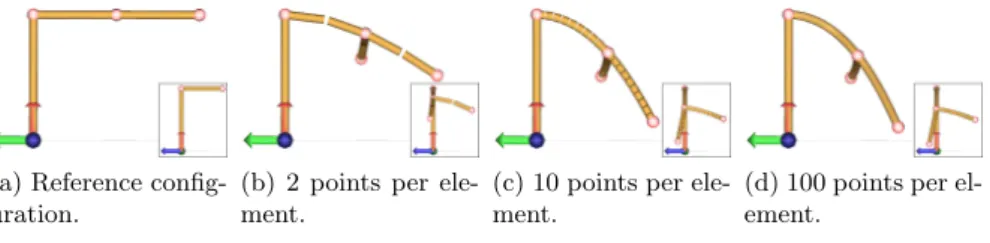
We first tested our algorithm on a simple branching system composed of a rigid trunk, a horizontal branch and a secondary branch borne by the former one. The method is able to account for bending and twist, Fig. 7. Only few nodes were needed (here, only at each end of the branch and at each of its ramification nodes) to obtain curvature along the axis (Fig. 7d). Note that if we do not have enough integration points (Fig. 7b), the number of nodes and integration points are not enough to converge correctly.
To analyze this resolution issue, we compared our result to the model pre-sented in the section 2 (green curves in Fig. 8). We present two simulations:
(a) Reference config-uration.
(b) 2 points per ele-ment.
(c) 10 points per ele-ment.
(d) 100 points per el-ement.
Fig. 7. Branch bending with one ramification. 1 node (red spheres) at each end and ramification. Integration points are located on the midpoint of each brown segment (integration areas).
– one with only two nodes (at the beginning and at the end of the axis): we are only varying the number of integration points (blue curves in Fig. 8), – another one where we are varying the number of nodes and where the number
of integration points per element is fixed to 10 (red curves in Fig. 8).
(a) Execution time (in seconds) as function of integration points num-ber (in FDM, integration points and nodes numbers are the same).
(b) Convergence (norm of the de-flection) as function of nodes num-ber except for blue curve: as func-tion of integrafunc-tion points number. Fig. 8. Performances of our method on a single axis bending compared to FDM (refer-ence mode, green curves). Two approaches are studied: nodes number fixed and increase the points integration numbers (2 nodes, blue curves) ; increase nodes number with fixed integration points number per element (red curves).
Fig. 8a shows us that our method is faster than a finite di↵erence method. In general, the execution time increases roughly linearly with the number of integration points. Furthermore, for a given number of integration points, the less nodes we use the faster is our method.On Fig. 8b, we observe that our method converges more rapidly than a FDM method for a similar number of nodes. The error (distance between the simulated and the theoretical values) is a decreasing function of number of nodes. However, decreasing the number of integration points does not change the convergence speed but may a↵ect the
convergence itself (blue curve). A minimal density of integration points must therefore be used to obtain correct physical results.
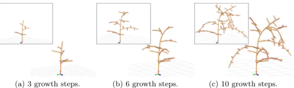
Our method allows to compute branch bending with di↵erent kinds of growth rules (Fig. 9): we can play with reference curvature, material properties (density, Young and shear modulii, . . . ), order of ramifications, children number at each ramification, sections, segment’s length. . .
(a) 3 growth steps. (b) 6 growth steps. (c) 10 growth steps. Fig. 9. Branch bending on growing tree with 2 perspectives.
5
Conclusion
In this paper, we extended FDM to FEM integration in L-systems. For this we had to use a multiscale approach where the plant is represented at two scales to model both the nodes and the integration points of a FEM approach. We showed that we could solve symmetric and definite positive linear systems thanks to a Cholesky decomposition in L-systems, that made it possible to use the branching structure itself to propagate the numerical integration as a flow of information from the basis of the plant to the tip and reciprocally.
Our comparative analysis showed that our L-system FEM converges more rapidly for our application than L-system FDM (with same model). This ap-proach, illustrated on a mechanical problem of branch bending, can be readily extended to the resolution of other systems involving di↵erential equations on branching systems.
References
1. Allen, M. and Prusinkiewicz, P. and DeJong, T. M.: Using L-systems for mod-eling source-sink interactions, architecture and physiology of growing trees: the L-PEACH Model. New Phyotologist 166, 869–880 (2005)
2. Bathe, K.: Finite Element Procedures. Prentice Hall (1996)
3. Boudon, F. and Pradal, C. and Cokelaer, T. and Prusinkiewicz, P., and Godin, C.: L-Py: an L-system simulation framework for modeling plant architecture develop-ment base on a dynamic language. Frontiers in Plant Science 3(76) (2012)
4. Chou, P. C. and Pagano, N. J.: Elasticity: tensor, dyadic, and engineering ap-proaches. Courier Dover Publications (1992)
5. Costes, E. and Smith, C. and Renton, M. and Gu´edon, Y. and Prusinkiewicz, P. and Godin, C.: MAppleT: simulation of apple tree development using mixed stochastic and biomechanical models. Functional Plant Biology 35(10) (2008) 6. Featherstone, R.: Efficient Factorization of the Joint-Space Inertia Matrix for
Branched Kinematic Trees. The International Journal of Robotics Research 24(6), 487–500 (2005)
7. Federl, P. and Prusinkiewicz, P.: Solving di↵erential equations in developmental models of multicellular structures expressed using L-systems. Computational Sci-ence – ICCS 2004 pp. 65–72 (2004)
8. Godin, C. and Sinoquet, H.: Functional-structural plant modelling. The New Phy-tologist 166(3), 705–708 (2005)
9. Hemmerling, R. and Evers, J. B. and Smoleov, K. and Buck-Sorlin, G. and Kurth, W.: Extension of the GroIMP modelling platform to allow easy specification of dif-ferential equations describing biological processes within plant models. Computers and Electronics in Agriculture 92(C), 1–8 (2013)
10. Jirasek, C. and Prusinkiewicz, P. and Moulia, B.: Integrating biomechanics into developmental plant models expressed using L-systems. Plant Biomechanics 24(9), 614–624 (2000)
11. Peir´o, J. and Sherwin, S.: Finite Di↵erence, Finite Element and Finite Volume Methods for Partial Di↵erential Equations. Dordrecht: Springer Netherlands Hand-book of Materials Modeling, 2415–2446 (2005)
12. Press, W. H., and Teukolsky, S. A. and Vettering, W. T. and Flannery, B. P.: Numerical Recipes: The art of scientific computing. Cambridge University Press (1987)
13. Prusinkiewicz, P.: Geometric modeling without coordinates and indices. IEEE Computer society Proceedings of the IEEE Shape Modeling International., 3–4 (2002)
14. Prusinkiewicz, P.: Modeling plant growth and development. Current Opinion in Plant Biology 7(1), 79–83 (2004)
15. Prusinkiewicz, P. and Allen, M. and Escobar-Gutierrez, A. and DeJong, T. M.: Numerical methods for transport-resistance sink-source allocation models. Frontis 22, 123–137 (2007)
16. Prusinkiewicz, P. and Lindenmayer, A.: The algorithmic beauty of plants. Springer (1990)
17. Prusinkiewicz, P. and Runions, A.: Computational models of plant development and form. The New Phytologist 193(3), 549–569 (2012)
18. Taylor-Hell, J.: Incorporating biomechanics into architectural tree models. Com-puter Graphics and Image Processing SIBGRAPI 2005. 18th Brazilian Symposium on. IEEE (2005)
19. Vos, J. and Evers, J. B. and Buck-Sorlin, G. H. and Andrieu, B. and Chelle, M. and de Visser, P. H. B.: Functional-structural plant modelling: a new versatile tool in crop science. Journal of Experimental Botany 61(8), 2101–2115 (2010)
![Fig. 1. Branch represented L-string I I [ I I ] I [ I ] I with information x = 1 (red segments) propagation to others segments (blue).](https://thumb-eu.123doks.com/thumbv2/123doknet/13924525.450053/3.892.299.627.504.616/fig-branch-represented-string-information-segments-propagation-segments.webp)