Application of genetic algorithm and deep reinforcement learning for in-core fuel management

Application of Genetic Algorithm and Deep Reinforcement Learning for In-Core Fuel Management

by Jane C. Reed

Submitted to the Department of Nuclear Science and Engineering in partial fulfillment of the requirements for the degree of

Bachelor of Science in Nuclear Science and Engineering at the

Massachusetts Institute of Technology May 2020

© Jane Reed All Rights Reserved

The author hereby grants to MIT permission to reproduce and to

distribute publicly paper and electronic copies of this thesis document in whole or in part in any medium now known or hereafter created.

Signature of Author: ……….

Jane Reed

Department of Nuclear Science and Engineering 05/15/2020 Certified by: ………...

Koroush Shirvan

Assistant Professor of Nuclear Science and Engineering Thesis Supervisor

Accepted By:………

Michael Short

Associate Professor of Nuclear Science and Engnieering Undergraduate Chair

Application of Genetic Algorithm and Deep Reinforcement

Learning for In-Core Fuel Management

Jane

Reed

Submitted to the Department of Nuclear Science and Engineering in partial

fulfillment of the requirements for the degree of Bachelor of Science in Nuclear

Science and Engineering

Abstract

The nuclear reactor core is composed of few hundred assemblies. The loading of these assemblies is done with the goal of reducing its overall cost while maintaining safety limits. Typically, the core designers choose a unique position and fuel enrichment for each assembly through use of expert judgement. In this thesis, alternatives to the current core reload design process are explored. Genetic algorithm and deep Q-learning are applied in an attempt to reduce core design time and improve the final core layout. The reference core represents a 4-loop pressurized water reactor where fixed number of fuel enrichments and burnable poison distributions are assumed. The algorithms automatically shuffles the assembly positions to find the optimum loading pattern. It is determined that both algorithms are able to successfully start with a poorly performing core loading pattern and discover a well performing one, by the metrics of boron concentration, cycle exposure, enthalpy-rise factor, and pin power peaking. This shows potential for further applications of these algorithms for core design with a more expanded search space.

Contents

1 Introduction...5 1.2 Objectives ...6 2 Background ...7 2.1 SIMULATE and CASMO ...7 2.2 Genetic Algorithm ...7 2.3 Deep Q Learning ...7 3 Methodology ... 11 3.1 Core Set-Up... 11 3.2 Core Depletion ... 11 3.3 Constraints and Objective Function ... 12 3.4 Location Swapping ... 13 3.5 Implementing the Genetic Algorithm (GA) ... 14 3.6 Implementing Deep Q Learning (DQN) ... 15 3.7 Hyperparameter Tuning in Tune... 15 4. Results ... 17 4.1 GA and DQN... 17 4.2 Further Investigation ... 20 5. Bibliography ... 21

Figures

Figure 1: Q-learning algorithm. Exactly reproduced from [5]. ...8 Figure 2: DQN Algorithm [9] ... 10 Figure 3: Example core reload pattern. ... 12 Figure 4: Ordered crossover in the genetic algorithm ... 14 Figure 5: Initial core layout (left) and final core layout (right) ... 17 Figure 6: Exposure distribution of optimal core layout ... 19 Figure 7: Objective function convergence for DQN (left) and GA (right) ... 19

1 Introduction

For an electric nuclear utility company, operational cost of a nuclear reactor is a costly endeavor. Thus, any methods for lowering the cost while preserving reactor safety are highly attractive. One key determinant of the economics of a reactor is the nuclear fuel management. There are two types of fuel management: in-core and out-of-core [1]. Out-of-core fuel management involves the decision of what kinds of fuel to use and how to manage them inside the spent fuel pool. In-core fuel management, which will be the focus of this thesis, involves the spatial arrangement of the chosen fuel assemblies in the nuclear reactor core.

The challenge with determining an in-core fuel distribution is that there is an enormous number of possible layouts for the fuel. The computational cost is proportional to O(n!) where n is number of fuel assemblies to shuffle, 10193 in this case [2], so it would not be feasible for us to test all possibilities. Originally, layouts were developed by hand and tested one at a time with limited computational power. This process led to designs which were conservative in power peaking, typically achieved by placing all fresh fuel assemblies on the edge of the reactor [1]. Economically, this was not an efficient design, as it was choice primarily dictated by safety considerations. By the 1980s, highly accurate and computationally efficient reactor simulations (e.g. CASMO and SIMULATE) were developed that allowed in-core fuel management to be done less conservatively with regards to safety, while in some cases testing a wider variety through stochastically-developed fuel management algorithms or decision making. This is how core design is performed today. However, this method is still limited in that inputs to the simulation are confined to what the current stochastic algorithms can produce. This is nowhere near the total amount of possible layouts that would be able to be tested. Once a good pattern is found, core designers typically keep the future loadings the same. This may result in core designers settling on a local optima of fuel layouts rather than the global optima.

However, given the recent developments in machine learning algorithms, there exists potential for finding a better optimum. Two algorithms— genetic algorithm (GA) and deep Q-learning (DQN)— may enable core designers to more effectively search the space of core layouts for the ideal layout.

1.2 Objectives

In the field of reactor core optimization, it is standard to construct arrangements of fuel assemblies using stochastic algorithms and test with core simulation programs. This leads to inefficiencies in the form of sub-optimal fuel layouts and unnecessary time spent on core design. Given recent advancements in machine learning, these inefficiencies may be eliminated. Using the GA and DQN methods, one may be able to test a large variety of fuel layouts in a fully automated fashion, ideally converging towards a global optimum. This algorithm could be more likely to find a global optimum than traditional approaches. If implemented successfully, it may be possible to find a better fuel layout than those found by core engineers, saving companies time and money on core design and reactor fuel costs.

2 Background

2.1 SIMULATE and CASMO

The simulation of the reactor core is performed using two tools, “CASMO” and “SIMULATE”. CASMO is a lattice physics code for modeling PWR’s and BWR’s. CASMO was used to simulate the different types of fuel assemblies involved in the example core using 2D lattice physics. CASMO generates the homogenized nuclear cross-section libraries for all fuel assembly types to be used in the core simulation. Once the assemblies were simulated in CASMO, SIMULATE was used as a core simulator, to assemble the full core and run it through fuel depletion cycles, shuffling fuel in between cycles. Specifically, CASMO4e with ENDFVI cross section library and SIMULATE3 were used in this work.

2.2 Genetic Algorithm

A genetic algorithm is not quite machine learning, but rather, a search heuristic modeled on Charles Darwin’s theory of evolution [3]. It aims to mimic the process of natural selection, in which the fittest individuals are enabled to “breed” and advance their genetic material to the next generation. It makes use of biologically inspired operators such as selection, crossover, and mutation to “breed” the fittest individual.

In order to run a genetic algorithm, it is necessary to first establish an initial population of individuals with randomized characteristics. Next, these individuals will be evaluated on their fitness using an objective function (also known as the fitness function). The fittest individuals are stochastically selected to breed with another fit individual, and experience genetic crossover and possibly point mutations. The children of these fittest pairs make up the second generation. The algorithm generally terminates when a maximum number of generations has been reached or a desired level of fitness is attained.

2.3 Deep Q Learning

Reinforcement learning is a type of machine learning that focuses on training an agent to maximize reward by taking a sequence of actions as it explores an environment. In simpler terms,

it is a method to train an agent to take a “good” sequence of actions in an environment it initially knows nothing about. In the context of the fuel loading optimization problem, the agent needs to learn the best sequence of fuel assembly swaps to create the optimal core.

Successful reinforcement learning is achieved through the continuous update of “Q-values” of different state action pairs. Q-values are ideally a representation of how useful an action is in a given state of a system. They not only consider immediate reward from the state-action pair, but also potential rewards from the future actions. A typical Q-value update is shown in Equation 1, otherwise known as the Bellman Equation.

𝑄[𝑠, 𝑎] = (1 − 𝛼)𝑄[𝑠, 𝑎] + 𝛼(𝑟 + 𝛾 max 34 𝑄[𝑠

5_{, 𝑎}5_]) Equation 1

Here, 𝛼 represents the “learning rate” of the system. It is a measure of how much you weight the old Q-value vs. the update to the Q-value, and is often set to 0.5. 𝛾 here is referred to as the “discount factor”, and sets how much the system discounts the value of future Q’s vs. the current reward it has found. However, this is simply the update to Q-value, and must be embedded in a larger algorithm in order to perform Q-learning.

Figure 1: Q-learning algorithm. Exactly reproduced from [5].

In this algorithm, the action “a” is selected via the function “select_action”. This function is typically executing an 𝜖-greedy strategy. In an 𝜖-greedy strategy, with probability 1 – 𝜖 the agent

selects the Q-value maximizing action, and with probability 𝜖 the agent selects an action at random. This stochastic element of the algorithm allows the agent to more fully explore its environment. Eventually, the agent should ideally be able to discern the best set of actions in its environment by experiencing the environments rewards for different actions. However, Q-learning alone is not an appropriate solution for the fuel arrangement problem, because there are far too many state-action pairs for the agent to learn them all.

Deep Q-learning combines both deep learning (neural nets) and Q-learning to train agents to navigate the expansive environments efficiently [6]. In deep Q-learning, the Bellman Equation is no longer computed explicitly, as to store and access all Q-values in a table would be far too computationally expensive. Instead, a neural network is used to compute the Q-value for each state-action pair based on observation. However, a single neural network is not enough, because the system experiences a single point at a time, which can lead to overfitting.Instead, DQN makes use of two networks— a training network and a prediction network. The training network, also known as the primary Q network, is updated every step. The prediction network, known as the target network, is only updated after a fixed number of steps C. The objective is to minimize the difference between the prediction of the target network and that of the primary network, as seen in Equation 2 𝐿𝑜𝑠𝑠 = :;𝑟_<+ 𝛾 max =4 𝑄(𝑠<>?, 𝑎 5_{; 𝜃̅)C − 𝑄(𝑠} <, 𝑎<; 𝜃)D E Equation 2

in which 𝜃̅ refers to the target network and 𝜃 to the primary, and 𝑘 index refers to the next item in the replay memory. Note that the action 𝑎′ is selected with the primary network and the Q value is evaluated using the target network. This is to prohibit systematic overestimation, as first established by Hasselt et al. [8]. Additionally, tuning C is essential for a stable DQN. Small C values imply too frequent updates of the target network which could lead to instabilities earlier in training. Also, large C values imply less updates, which can lead to a poor accuracy (i.e. large Loss) in the final model.

The algorithm is included in Figure 2 below. It begins by setting hyperparameters 𝜖_HIHJ, 𝜖KIL, 𝐶, 𝐵, 𝑁P=QRST, and 𝑁=IIK=U . As in Q-learning, 𝜖 establishes the balance between exploration and exploitation in the environment. However, in DQN, 𝜖 decreases slowly over time, causing less exploration by the end of the training period. The length of this training period is

established with 𝑁_=IIK=U. Replay memory, 𝐷, stores experiences in a buffer during training and 𝑁_P=QRST initializes the memory with random actions. Next, a set number of time steps are executed, which are grouped into episodes, which are then grouped into epochs. The purpose of the epochs is to average several episodes and determine the mean reward, as well as other useful statistics such as the standard deviation, max, and min. If the model is an improvement, it is saved.

3 Methodology

3.1 Core Set-Up

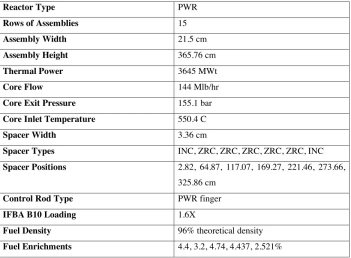
Prior to beginning the optimization of a reactor core, it was necessary to establish the reference core. In this case, a typical 4-loop PWR core with the following specifications was modeled: Table 1: Core Specifications Reactor Type PWR Rows of Assemblies 15 Assembly Width 21.5 cm Assembly Height 365.76 cm Thermal Power 3645 MWt Core Flow 144 Mlb/hr

Core Exit Pressure 155.1 bar

Core Inlet Temperature 550.4 C

Spacer Width 3.36 cm

Spacer Types INC, ZRC, ZRC, ZRC, ZRC, ZRC, INC

Spacer Positions 2.82, 64.87, 117.07, 169.27, 221.46, 273.66,

325.86 cm

Control Rod Type PWR finger

IFBA B10 Loading 1.6X

Fuel Density 96% theoretical density

Fuel Enrichments 4.4, 3.2, 4.74, 4.437, 2.521%

For a more detailed description of the exact layout of each fuel type used, and the layout of the top, bottom, and radial reflectors, please see the attached CASMO input files.

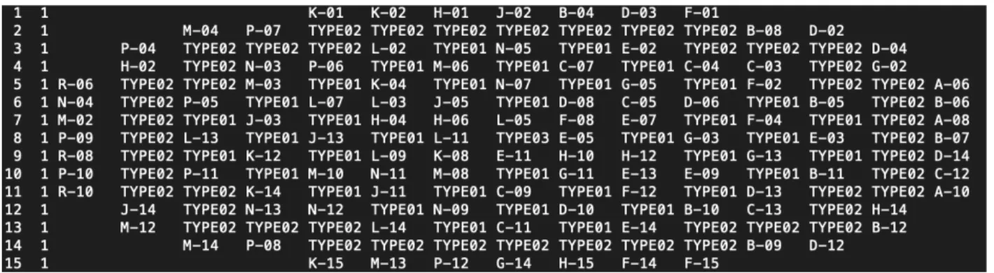
With the core specifications established in SIMULATE, it was then necessary to deplete the core, i.e. simulate fission reaction and thermal energy extraction from the core. The time from which the core starts and finishes is referred to as a “cycle”. During the cycle, SIMUALTE calculates the critical boron concentration, .i.e. the concentration of boron in the coolant that allows the fission reacting in the core to continue. The end of cycle is characterized when the coolant boron concentration reaches zero, .i.e. there is not enough reactivity in the fuel to keep the fission chain reaction going. After a single depletion cycle of 28 GWD/MT, the core reload composed of 36 assemblies of TYPE01 fuel (enrichment 4.437%, IFBA coated), 48 assemblies of TYPE02 fuel (enrichment 4.4%, IFBA coated), and 1 assembly of TYPE03 fuel (enrichment 2.521%, IFBA coated). These new assemblies that are loaded during every cycle are typically called Fresh assemblies. The one that remain from the previous cycle, are called “once-burned” assemblies. Some assemblies remain in the core for a third cycle and they are called “twice-burned”. See Figure 3 for an example of fuel loading at the beginning of a new cycle.

Figure 3: Example core reload pattern.

3.3 Constraints and Objective Function

In order to evaluate the performance of the reactor core loading pattern, the reactor was analyzed using a few metrics:

Table 2: Constraints for loading pattern performance

Metric Feasible Value Optimal Value

Boron Concentration < 1300 ppm < 1175 ppm

Exposure < 62 GWD/MTU < 62 GWD/MTU

F-delta-H < 1.58 < 1.48

For the objective function, the optimal values were used to penalize solutions which exceed these values. Score was determine by:

𝑠𝑐𝑜𝑟𝑒 = 𝑒𝑥𝑝𝑜𝑠𝑢𝑟𝑒 − (𝑐_\]Q]I+ 𝑐_{K^T]_SQK}+ 𝑐_TK=<HI`+ 𝑐_aLKUJ=b) Equation 3 where 𝑐_^ = 𝑤 :𝑥Q=P− 𝑥]TJHR=U 𝑥]TJHR=U D E Equation 4

and w = 500 for boron, peaking, and F-delta-H, and 1000 for exposure. This format of objective function allows us to search for solutions which come as close as possible to 62 GWD/MT exposure without exceeding it, and minimize boron concentration, max peaking factor, and F-delta-H.

3.4 Location Swapping

In order to run both GA and DQN on the core, it was first needed to establish some method of assembly shuffling which would allow us to look at a large variety of possible core layouts. Because of the symmetry in the fuel layout, the assembly swapping was constrained to one quarter of the full core, and replicated the same swapping pattern throughout the other three quarters of the core. Due to limitations on the computing power and time, it was decided to shuffle only the first 16 out the 41 locations of the quarter core as an attempt at proof of concept for the optimization algorithms. This number was chosen empirically as it allowed us to run the simulation in a reasonable amount of time for debugging. Additionally, the number of possible combinations of 16 assemblies (16! = 2.09E13) is a good balance between a high dimensional space to test the performance of the algorithms and the available computing power. In fact, due to restrictions on fuel assembly placement (such as no fresh fuel assemblies being permitted on the periphery of the core) there are closer to just two million possible arrangements. Ideally, however, with large computing time and resources wider design spaces can be explored.

3.5 Implementing the Genetic Algorithm (GA)

The genetic algorithm was implemented using Distributed Evolutionary Algorithms in Python, or DEAP [7]. Using this package, it was simply needed to determine hyperparameter values, and adapt the processes of genetic algorithm to the specific example. In this case, the hyperparameters that were needed to determine were the probability of a swap (on the order of 0.05), the probability of a mutation (on the order of 0.05), and the probability of a crossover (on the order of 0.5). It was also needed to determine an appropriate number of individuals in each generation and the appropriate number of generations, which we did using the “tune” algorithm that we explain in Section 3.7.

In the context of the fuel layout in a reactor core, crossover between individuals is bit complicated. For an example, we will look at two possible vectors of assembly positions

Parent 1: [4 1 13 3 14 5 6 7 15 9 10 11 12 2 0 8] Parent 2: [9 0 8 3 11 12 7 6 15 4 10 14 1 2 5 13]

Since only one copy of each individual assembly is needed, if the first half of parent 1 was combined with the second half of parent 2, it would result in an invalid vector. Therefore, an ordered crossover was used instead [4]. The ordered crossover works by randomly selecting a sequence of 8 assemblies from parent 1, eliminating those from parent two, and combining the remaining assemblies into the child.

Parent 1: [4 1 13 3 14 5 6 7 15 9 10 11 12 2 0 8] Parent 2: [9 0 8 3 11 12 7 6 15 4 10 14 1 2 5 13] Child: [0 8 3 12 14 5 6 7 15 9 10 11 4 1 2 13]

Figure 4: Ordered crossover in the genetic algorithm

This method allows to combine to vectors without repeating any assemblies.

Lastly, to evaluate the computation time necessary to perform GA, it is important to note that the number of calls to SIMULATE is equal to the number of individuals in each generation times the number of generations. Therefore, the smallest number of individuals and generations that can be useful is targeted.

3.6 Implementing Deep Q Learning (DQN)

The implementation of DQN in the case of the reference reactor core is fairly straightforward. The Stable Baselines package [4] was used in order to structure the DQN algorithm. It was then necessary to determine the optimal hyperparameters using “tune”. The best saved model is used for testing to find the best arrangement the model can produce, which is of high quality and should be better than the core pattern that initiated the optimization.

3.7 Hyperparameter Tuning in Tune

In the attempt to determine the optimal hyperparameters for both GA and DQN, it was necessary to perform some hyperparameter tuning. This was provided in the algorithm “tune”, which performs a grid search to determine the best hyperparameters. The grid search begins with the user establishing a narrow range of possible values for each hyperparameter. Next, the provided range is divided into k separate nodes, where more nodes are used for the sensitive hyperparameters to better explore the range. Next, all possible combinations of the hyperparameters are evaluated and the mean and maximum reward for each combination is recorded. Once this process is completed, the top performing combinations of hyperparameters may be selected to apply to the algorithm. When referring to tuning the hyperparameters using “tune” at any point in this thesis, this algorithm is being referenced. The tuning process is applied in this work for both DQN and GA.

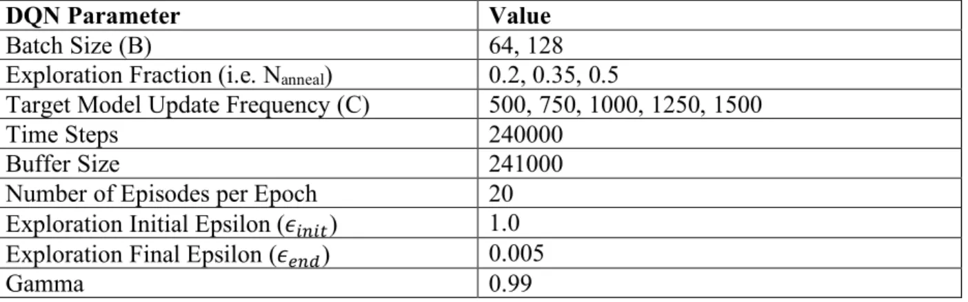
The hyperparameters which were tested are included below. Table 3: DQN Inputs

DQN Parameter Value

Batch Size (B) 64, 128

Exploration Fraction (i.e. Nanneal) 0.2, 0.35, 0.5

Target Model Update Frequency (C) 500, 750, 1000, 1250, 1500

Time Steps 240000

Buffer Size 241000

Number of Episodes per Epoch 20

Exploration Initial Epsilon (𝜖_HIHJ) 1.0 Exploration Final Epsilon (𝜖_KIL) 0.005

Warmup Steps (Nwarmup) 4800

Learning Rate 0.0005

Train Frequency 4

Double Q option True

Prioritized Replay option True

Prioritized Replay 𝛼 0.6 Prioritized Replay 𝛽 0.4 GA Parameter Value Crossover Probability 0.4, 0.6, 0.8 Initial Population 25, 50, 75 Number of Generations 200 Independent Probability 0.05, 0.1, 0.15 Mutation Probability 0.05, 0.1, 0.15

4. Results

4.1 GA and DQN

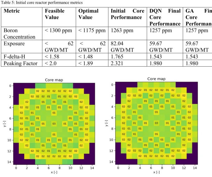
In order to execute the GA and DQN algorithms, an inefficient core that performed poorly on the metrics of interest was used as a starting point (see Table 5).

Table 5: Initial core reactor performance metrics

Metric Feasible Value Optimal Value Initial Core Performance DQN Final Core Performance GA Final Core Performance Boron Concentration < 1300 ppm < 1175 ppm 1263 ppm 1257 ppm 1257 ppm Exposure < 62 GWD/MT < 62 GWD/MT 82.04 GWD/MT 59.67 GWD/MT 59.67 GWD/MT F-delta-H < 1.58 < 1.48 1.765 1.543 1.543 Peaking Factor < 2.0 < 1.89 2.321 1.980 1.980 Figure 5: Initial core layout (left) and final core layout (right)

Then the range of hyperparameters over which to search for the optimal core layout were established. It was found that in the case of both DQN and GA, the performance was insensitive to hyperparameter tuning. This finding implies that the algorithm tends to converge to core patterns of similar quality, but with small effect from its hyperparameters. In addition, it is worth mentioning that advanced logging techniques during optimization were used to save every pattern investigated, and it was concluded that the optimization process yielded many core patterns of high

quality (i.e. whose objective values very close to the best pattern found). This means that DQN and GA have good exploratory behavior that can provide multiple options to the core designers for the simulated problem.

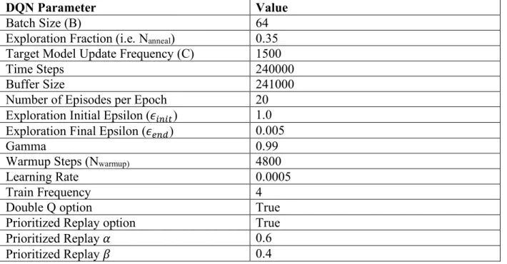
The best combination of hyperparameters are included in Tables 6 and 7, below. For DQN, the optimum value for exploration fraction of 0.35, i.e. it was spending 1/3 of the training time in exploration and the rest in exploitation.

Table 6: DQN Inputs

DQN Parameter Value

Batch Size (B) 64

Exploration Fraction (i.e. Nanneal) 0.35 Target Model Update Frequency (C) 1500

Time Steps 240000

Buffer Size 241000

Number of Episodes per Epoch 20

Exploration Initial Epsilon (𝜖_HIHJ) 1.0 Exploration Final Epsilon (𝜖_KIL) 0.005

Gamma 0.99

Warmup Steps (Nwarmup) 4800

Learning Rate 0.0005

Train Frequency 4

Double Q option True

Prioritized Replay option True

Prioritized Replay 𝛼 0.6 Prioritized Replay 𝛽 0.4 Table 7: GA Inputs GA Parameter Value Crossover Probability 0.6 Initial Population 40 Number of Generations 200 Independent Probability 0.05 Mutation Probability 0.15

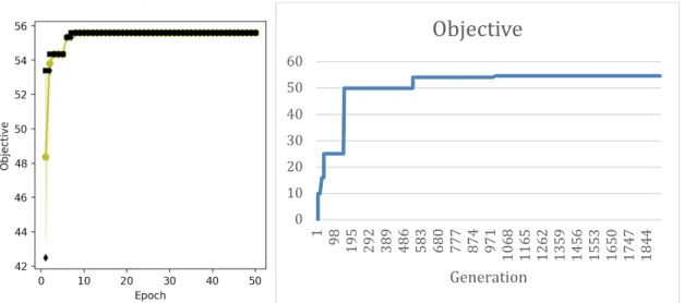
It can be seen from Table 5 that GA and DQN are in good agreement as they converged to the same objective value. In the case of DQN, the convergence to best objective occurred after about 10 epochs, which involved a total of 10 (epochs) × 20 (episodes) × 240 (time steps) =48000

SIMULATE calls. In the case of GA, about 1000 generations are needed to converge to the best core, which involved about 1000 (generations) × 40 (population) =40000 SIMULATE calls.

Figure 6: Exposure distribution of optimal core layout

Figure 7: Objective function convergence for DQN (left) and GA (right)

While the algorithms eventually converge to an improved core, it did not fully meet the optimal core targets, though it is unclear if the current problem setup can meet the targets. The results that were found proved that DQN and GA are viable machine learning options for core optimization. By having additional computing power and allowing larger search times, it is expected to find better results.

0 10 20 30 40 50 60 1 98 195 292 389 486 583 680 777 874 971 1068 116 5 126 2 135 9 145 6 155 3 165 0 174 7 184 4 Generation

Objective

4.2 Further Investigation

In the future, the goal would be to confirm that the DQN agent is actually performing assembly swaps in an intelligent manner. In this case, the stochastic nature of the algorithm leads to a quick discovery of a new and better core, but this work did not test the agent to see if it maintained some learning. It seems likely that the agent is struggling to find its way back to the best solution to explore the space around it. It is possible that the nature of the problem is such that following gradients of the Q-values does not provide us with any better results than a fully stochastic search, in which case the approach to optimization would have to be redesigned as a search problem. Therefore, the DQN performance is better described as an optimizer like GA rather than a learner. In future work, DQN will be trained to learn how to continuously swap the fuel assemblies to maximize the objective over all training states. This learning to optimize behavior is expected to improve the DQN performance over GA by accelerating the search process and perhaps leading to better core patterns.

5. Bibliography

[1] C. Haugen, “The Greedy Exhaustive Dual Binary Swap Methodology for Fuel Loading Optimization in PWR Reactors Using the poropy Reactor Optimization Tool,” Masters of Science Thesis, MIT, 2014

[2] J. Frenje, “Absolute measurements of neutron yields from DD and DT implosions at the OMEGA laser facility using CR-39 track detectors,” Review of Scientific Instruments, vol. 73 no. 7, 2002

[3] Mallawaarachchi, Vijini. “Introduction to Genetic Algorithms - Including Example

Code.” Medium, Towards Data Science, 1 Mar. 2020, towardsdatascience.com/introduction-to-genetic-algorithms-including-example-code-e396e98d8bf3.

[4] “Hill-a/Stable-Baselines.” GitHub, 12 May 2020, github.com/hill-a/stable-baselines. [5] MIT 6.036 Lecture Notes

[6] V. Mnih, et al. "Human-level control through deep reinforcement learning." Nature 518.7540 (2015): 529-533.

[7] F. Fortin, et al. "DEAP: Evolutionary algorithms made easy." Journal of Machine Learning

Research 13.70 (2012): 2171-2175.

[8] V. Hasselt, et al. "Deep reinforcement learning with double q-learning." Thirtieth AAAI conference on artificial intelligence. 2016.