An application of the A* search to trajectory optimization

An Application of the A* Search to

Trajectory Optimization

by

Craig K. Niiya

Captain, United States Air Force B.S., Mechanical Engineering

Carnegie-Mellon University

(1985)

Submitted to the

Department of Aeronautics and Astronautics in Partial Fulfillment of the Requirements

for the Degree of Master of Science

at the

Massachusetts Institute of Technology June 1990

© Craig K. Niiya, 1990. All Rights Reserved.

Signature of Author

Certified by

Departmentbf Aeonautics d Astronautics

Dr. Richard H. Battin, Thesis Supervisor Adjunct Professor of Aeronautics and Astronautics

Certified by

Edward V. Bergmann, Tecnical Supervisor The Charles Stark Draper Laboratory, Inc.

AcceDted by

MA:,,ACHUSETL.TS INST1UTIE

CF TrECH ,...GY

1

1990

Professor Haroll Y. Wachman, Chairman Departntental Graduate Committee

LIBRARIES

4%

An Application of the A* Search to

Trajectory Optimization

by

Craig K. Niiya

Captain, United States Air Force

Submitted to the Department of Aeronautics and Astronautics on 11 May 1990 in partial fulfillment of the requirements for the Degree of

Master of Science in Aeronautics and Astronautics

ABSTRACT

As space operations become more complex and ambitious, there is a corresponding increase in the sophistication required of on-board algorithms for proximity operations. Unmanned missions such as planetary probes require sophisticated algorithms to deal with evolving mission requirements and contingencies, where man-in-the-loop control will be impractical. Other future missions that require autonomy for safety or security reasons will also require intelligent on-board controllers. This effort discusses a structure for a

candidate proximity operations controller and provides initial development of an intelligent trajectory planner in three degrees of freedom using the A* Node Search technique.

Thesis Supervisor (MIT): Professor Richard H. Battin, Adjunct Professor of Aeronautics and Astronautics

Acknowledgements

I am deeply grateful to Dr. Richard H. Battin for the interest which he took not only in my thesis, but in me. Indeed, it seems certain that his goal of sharing an awe and love for Astrodynamics has been accomplished in many of his students; I am privileged to have been one of them. I am also greatly appreciative of the many efforts extended on my behalf

by Edward V. Bergmann, my Technical Supervisor at the Charles Stark Draper

Laboratory. His insights and guidance have proved to be more than beneficial to any success I have had in pursuit of this thesis--his help has been essential. John Raquet, who is continuing with efforts to pursue this application of A* technique further, has also volunteered his insights most graciously. More importantly, though, he is a good friend and a valued partner in the Gospel of Christ.

There are so many others at the Lab who have helped me with technical concepts, advice on presentation of my work, and who have, in short, been my friends, especially Todd Dierlam, Tony Bogner, Charles Cooke and Bruce Persson. As they say in Hawaii, Mahalo!--Thank you very much! I would also like to thank the lab for sponsoring this IR&D project and for providing this graduate fellowship which made my time here possible.

I also like to thank my many other friends that make up my church family, but in

particular--David Johnson, Matthew Ide, David Lucia, Bruce Fottler and Melody Martin, Paul Christensen, David Gibb, Jeff Sanders, Jeff Bishop, and Lynn Thornton. Your love, support, and encouragement have been outstanding, but your willingness to share your lives and friendship with me, your ability to be vulnerable with me has endeared this time to me. I am forever grateful that you are truly my family (Mt. 12:50). There are so many who have contributed to my growth as a person, as an Air Force Officer, and most importantly as a friend of Christ's--to all of you, "thank you" seems hardly enough.

Each of us has reason to be grateful simply for our birth. Those of us that are fortunate enough to have received nurturing, understanding and support from our parents and families owe an even greater debt of love and gratitude. To my parents, my brothers and their wives and my two nieces, I love you all and I thank my Lord for you. I know with certainty few things, but I know this for sure: your investments in my life have been and continue to be foundational in all that I am and shall ever be. I am profoundly grateful.

Finally, and most importantly, I thank the LORD, my God. It is through Christ that I find reason to live and through Him that I find the energy and direction for the many pursuits in which He leads; it is through His mercy and grace that I am forgiven. You have given me love, hope, and faith. It is only fitting that I give you my life (Romans 12:1).

This report was prepared at The Charles Stark Draper Laboratory, under Draper Independent Research and Development (IR&D). Publication of this report does not constitute approval by the Charles Stark Draper Laboratory or the Massachusetts Institute of Technology of the findings or conclusions contained herein. It is published solely for the exchange and stimulation of ideas.

I hereby assign my copyright of this thesis to The Charles Stark Draper Laboratory, Cambridge, Massachusetts.

Craig K. iy

Captain, US Air Force

Permission is hereby granted by The Charles Stark Draper Laboratory to the Massachusetts Institute of Technology to reproduce any or all of this thesis.

TABLE OF CONTENTS

1. Introduction

5

Proximity Operations

Extending Mission Capability and Autonomy Intelligent Planner

Optimal Control

Hybrid Control Strategy Outline

2. Background

13

Transfer Problems Hill's Equations

Derivation of Force-Free Hill's Equations The State Transition Matrix

A*Search

An Example of an A* Search

3. A*Search: Trajectory Planning with Anomalies

26

Grid Assignment Concepts Calculating the Cost Links to the Autopilot Implementation

4. Testing

43

The Simulation

Testing Description Test Cases

Case 1: Altitude Change Maneuver Case 2: V-Bar Maneuver

Case 3: In-Plane Maneuver Case4: Out-of-Plane Maneuver Multiple Obstacles

Comparison to a Two-Impulse Trajectory Solver Unplanned Disturbance

5.

Conclusions

64

Summary

Recommendations for Future Work

Appendix: Development of Solutions

71

Chapter 1. Introduction

1 INTRODUCTION

PROXIMITY OPERATIONS

Space missions frequently require tasks such as rendezvous, docking, or stationkeeping, commonly referred to as proximity operations. By nature, these

maneuvers are typically the most complicated and often the most fuel inefficient parts of the mission because of the high level of constraints placed on the motion of the vehicle.

Many current and future missions with vehicles such as the Space Transportation System (Space Shuttle) or the Orbital Maneuvering Vehicle (OMV) depend on safe and efficient proximity operations--the servicing or retrieval of satellites, or docking or

stationkeeping with other spacecraft such as the space telescope or space station.

Interplanetary missions such as the Mars Rover Sample and Return (MRSR) Mission will also depend on reliable proximity operations for mission success.

EXTENDING MISSION CAPABILITY AND AUTONOMY

Spacecraft and space structures are rapidly increasing in complexity while the performance requirements continue to evolve to increasingly ambitious levels. Vehicles

approaching a space structure may now be required to grapple a docking port located near "obstacles" such as solar arrays, antennae, or even inhabited appendages of the structure.

Servicing vehicles will increasingly be required to accomplish close rendezvous for retrieval of payloads for repair or return to Earth. Previous examples of such retrievals

Chapter 1. Introduction

include the Solar Max repair on STS-41C and the Long Duration Exposure Facility (LDEF) recovery on STS-32.

The planning / replanning of the maneuvers which make up safe and reliable close proximity operations are therefore becoming more demanding activities, requiring the development of additional algorithmic tools to extend existing capabilities in this area. The technological gap between need and capability is especially visible in plans for truly

autonomous vehicles where the problem-solving resources of man-in-the-loop control are unavailable. At present, the precision and flexibility required in proximity operations has been provided mainly by extensive training, simulation, and the resourcefulness of pilot and ground crews. However, unplanned events may force inherently inefficient trajectories to be followed in the absence of sophisticated replanning capabilities. In the case of jet failures, for example, the spacecraft commander might be constrained by procedure to go to a pre-planned, stable standoff point while earth based controllers would replan the operational trajectory. While in-flight replanning could have made use of spacecraft momentum prior to the failure, current operational policy might instead dictate that

movement toward the target should be actively nulled, or perhaps, reversed to achieve the safe standoff condition.

Autonomy will become an increasingly critical capability when considering

interplanetary missions such as the proposed Mars Rover Sample and Return (MRSR). In Martian orbit, the pilotless vehicle will have limited communication with its earth based controller due to the long signal delays between Earth and Mars. Earth-based replanning might be unavailable or impractical if an unplanned event (such as jet failure) occurred in Martian orbit; real-time command and control data will be unavailable since radio

Chapter 1. Introduction

Implementing an in-flight replanning capability would require efficient use of computational assets. Real-time computations would be required to produce feasible and safe trajectories. Consequently, algorithms which were numerically simple would best accommodate these stringent real-time requirements. Planning algorithms which could also account for and possibly even take advantage of geometrical irregularities (such as effector coupling or spacecraft shape) could also contribute large dividends in fuel economy as well as time efficiency.

There is, then, a clear need to extend guidance and control systems capabilities for truly autonomous mission planning and implementation of safe and reliable control policies in real time.

INTELLIGENT PLANNER

In the case of the Space Shuttle, very specific automatic maneuvers have been implemented for attitude control; translational maneuvers, however, are still executed manually. While a preliminary automated docking controller concept has been investigated, it is severely constrained by pre-specified initial conditions [1]. In European and Soviet efforts towards autonomous control, nominal cases are programmed with a level of robustness. The controller takes the form of a regulator, keeping the vehicle close to a nominal trajectory. If excessive variations arise in initial conditions, vehicle performance, or environmental constraints, that violate some pre-specified region of tolerance, the control system will typically resort to achieving a safe standoff location where replanning efforts can be directed by Earth-based controllers [2]. The degree of autonomy is clearly linked to the degree of fault accommodation and robustness to variations in mission, vehicle and environmental parameters and constraints.

Chapter 1. Introduction

Unforeseen events such as malfunctions or off-nominal performance of a target vehicle could pose an extremely challenging docking task. The unpredictable motion of a disabled vehicle makes this type of "obstacle" a constraint that must be monitored and accommodated in real-time. While collision detection software does exist, that predicts location, time to impact, and type of collision [3], a unified approach to reconciling this data with other mission objectives and constraints has not previously been developed and implemented for on-board applications.

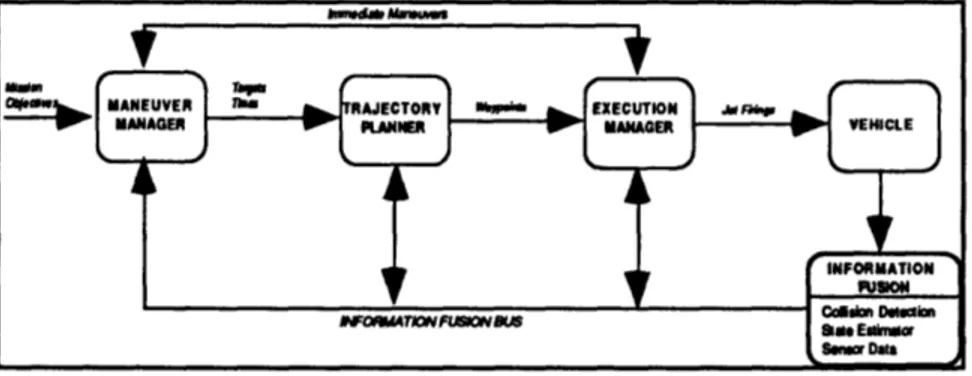
The planning architecture referred to in this thesis was envisioned to consolidate technology in automated maneuvers, collision prediction, and autopilot control systems to form an autonomous hierarchical planner [4]. The Autonomous Proximity Operations Planning System (APOPS), shown in Figure 1-1, uses three levels of decision

responsibility with corresponding levels of mission authority. The Maneuver Manager (MM) makes executive (or strategic) decisions, the Trajectory Planner (TP) accomplishes policy (or tactical) decisions, and the Execution Manager (EM) implements policy within a

specified cost horizon.

Figure 1-1. Three Tier Management

MANEUVER MANAGER

The Maneuver Manager (MM) considers the strategic decisions associated with mission execution. In the face of changing requirements, vehicle status, or environment,

Chapter 1. Introduction

the MM would choose whether to suspend execution of the current trajectory plan, to issue a work-around plan, or to stop and achieve a stable point to completely replan the

operation. Based on a perceived advantage or need to replan a trajectory (e.g. an

unforeseen obstruction to the current trajectory is detected by vehicle sensors), MM verifies that there is enough time to replan, and sends the Trajectory Planner a request for a new trajectory.

While the other two segments of this autonomous system would contain some algorithmic intelligence, MM would likely be the most dependent on programmed logic. A rule-based system could be an effective implementation of this logic since MM's decisions would be based on readily available and quantifiable information such as time to possible collision and jet performance / failure status. In response to this data, available through Information Fusion, MM logic would "optimize" the planner's performance by setting parameters such as grid meshsize or control effort granularity. Efficiency of computational effort may indeed be the difference between achieving the in-flight replanning capability and settling for the less efficient solution of moving to a stable standoff point and waiting for a new plan from the ground.

TRAJECTORY PLANNER

When requested by the MM, the Trajectory Planner (TP) will execute a search for an optimal or near-optimal control policy which will safely take the spacecraft from its current trajectory to a desired target while accommodating mission, vehicle, and

environment constraints. The TP makes decisions that may be considered "tactical" in the mission. Generating a waypoint string, an Optimal Search Algorithm (OSA) considers the orbital mechanics, the spacecraft dynamics, obstacle avoidance, vehicle control, and vehicle configuration status.

Chapter 1. Introduction

There is a tacit assumption that, prior to prompting the Trajectory Planner, the MM is monitoring the execution of a policy which is optimal under current circumstances. Responding to a change in vehicle status, mission requirements, or environment, MM requests a replanning effort and TP initiates a search for a neighboring optimal control policy, accounting for new or changing constraints. Using fuel expenditure as the main component of the performance measure, the OSA compares various trajectory alternatives to arrive at a suitable control policy, in the form of a waypoint string. This string is then placed in an information buffer which is accessed by the next tier manager--the Execution Manager.

EXECUTION MANAGER

The Execution Manager (EM) takes the trajectory solution generated by TP and generates control signals through a digital autopilot (DAP). The EM includes sensors and actuators as well as control logic. It is responsible for implementing the policies as directed by the higher managers. Along with data from the collision detector, Information Fusion receives information from the EM to generate vehicle and environment status reports as feedback to MM and TP.

OPTIMAL CONTROL

The optimal control of any process requires a performance measure and will typically need to satisfy state and control constraints. For a given spacecraft design, payload or maneuvering capacity is mainly determined by fuel considerations. Thus, the performance measure should serve to minimize fuel expenditures. Also, while transfer times are not fixed, it may be desirable to minimize the maneuver interval as well.

Constraints on state and control variables are mainly generated by safety concerns (such as vehicular collisions and plume impingement) and vehicle capabilities (i.e. jet authority).

Chapter 1. Introduction

HYBRID CONTROL STRATEGY

While traditional optimal control techniques can develop off-line policies which are optimal or near optimal, typically the computation required of such algorithms will render them impractical for autonomous proximity operations where in-flight mission planning is desired. In real-time, where faster algorithms are needed, heuristic node search techniques employing simple numerical operations can be used to obtain neighboring near-optimal control. Further, by exploiting parallel processing technology, the efficiency of these algorithms could be significantly enhanced.

While a node search technique could independently derive a refined optimal or near optimal control, it would then require an extensive node space, yielding again, an

impractical algorithm. A more efficient planner concept would use a traditional optimal control technique to develop a nominally optimal trajectory off-line while in-situ replanning would be accomplished by a node search technique to develop neighboring near-optimal solutions in the presence of evolving mission uncertainties and constraints. It is toward this strategy that we have developed the A* trajectory planner concept .

OUTLINE

This effort to implement an intelligent planner concept incorporates a linearized model of orbital motion called the Clohessy-Wiltshire Equations and a node search

technique called A*. The planner discussed in this thesis starts with a transfer time which represents a nominally optimal two-burn trajectory. It pieces together a multi-segment trajectory which avoids obstacles and accounts for vehicular limitations by using penalty functions on node costs.

Chapter 1. Introduction

Previous work has been done to implement the hierarchical planner concept and the A* search logic in the area of tactical aircraft mission planning [5,6]. Building from that experience, this thesis seeks to implement the A* search algorithm in the close proximity

operations area using an innovative node generation scheme to accommodate vehicle capabilities and evolving physical constraints.

Chapter 2. Background

2 BACKGROUND

TRANSFER PROBLEMS

Past research has investigated restricted transfer problems in Orbital Mechanics. Two problems which have received considerable study are the Hohmann Transfer and Lambert's Problem. The Hohmann Transfer is a fuel optimal transfer in altitude which does not allow arbitrary specification of phasing constraints or transfer time. The Hohmann Transfer moves a satellite from a circular orbit to a coplanar circular orbit at a

different altitude as the vehicle moves through half an orbit [7]. Because the Hohmann Transfer is a solution to a very specific problem, in the past, orbital maneuvers might have been planned in one of two ways. Solving the altitude change first, the phasing adjustment would be accomplished with a V-bar maneuver, providing a very stable approach to the target. A second approach might be to target an altitude above or below the target to accomplish phasing. If the target was behind of the chase vehicle, a higher orbit would be targeted and orbital mechanics would cause the chase vehicle to fall back relative to the target. The opposite would be done if the target was ahead of the chase vehicle.

Lambert's problem has also received considerable attention. It deals with the transfer of a vehicle from one orbit to another with phasing and time specified. There are an infinity of trajectories between two points on different orbits, varying only by transfer time (and correspondingly, orbital energy). However, a transfer is uniquely specified given the locations of the two endpoints and the transfer time [8].

This trajectory planner seeks a unique solution to the less constrained problem which calls for an optimal transfer between specified initial and terminal states while transfer time is left unspecified.

Chapter 2. Background

HILL'S (CLOHESSY-WILTSHIRE) EQUATIONS

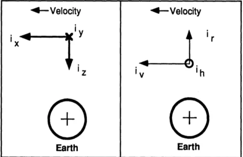
The Euler-Hill equations describe motion in the three translational degrees of freedom for proximity operations. The force-free solution of these equations have become known as the Clohessy-Wiltshire equations. The coordinate system used in this thesis is

commonly referred to as Local Vertical, Local Horizontal or LVLH reference frame; it is a simple rotation of the Hill's coordinate system. (See Figure 2-1.)

--

Velocity

Earth

-4

Velocity

Earth

Figure 2-1. LVLH, Hill's Coordinate Systems

Two of the three translational components i x, the unit vector along the velocity vector, and i z, the unit vector pointing to the center of attraction, are defined within the orbital plane while the third, i y, is the unit vector opposite the orbit angular momentum vector.

DERIVATION OF FORCE-FREE HILL'S EQUATIONS [9]

Newton's second law for a body's motion defined in a inertial frame of reference states that the acceleration of that body will be determined by the sum of the forces on the body.

Chapter 2. Background

i

=

We will assume that the jets used to achieve velocity changes are impulsive and that these equations of motion will be used to describe motion between these impulsive burns. Thus equation 2.1 reduces to:

= GMEarth r -- 2 r

.3

<2.2>

Making the change of coordinates to the LVLH frame we observe the following definitions:

1) let p be the position vector of a point in the LVLH frame:

p=xi + yj + zk

2) let co be the orbit angular momentum vector in the LVLH frame:

NOTE: o is a constant since we assume a circular orbit.

We have the relative velocity in the LVLH frame given by:

dp

VLVLH =

_dt

+ (o x p)

where the time derivative represents only the time rate of change in position within the reference frame and does not account for the motion of the coordinate system.

Expansion of equation 2.3 results in:

LVVLH = (x+Coz)i +

yj

Chapter 2. Background

The inertial acceleration is given by:

dVERTIA LVLH + (0) x VLVLH) + aLVLH <2.4>

dt

where the acceleration, aLVLH, is the centripetal acceleration of a body in circular motion,

given by o2R (R = nominal orbital radius for the origin of the LVLH frame).

aINERTIAL = (K+2oi-ox)i + yj +(i+2m(-ow2 +02R)k <2.5>

Expressing equation 2.2 into LVLH coordinates we find:

(=

(4x2 +

y (z-R)2

We now make some simplifying assumptions to linearize these expressions.

Noting that p << R, the magnitude of the acceleration components in the i and j directions can be well approximated by:

x=- GMEARTH x --C-Ix <2.6a> R3

and,

yn = GMEARTH y

_0

R3

However, in the k direction this approximation is not sufficiently accurate. To find a useful approximation, we use the binomial series to expand the expression. The expansion formula is:

Chapter 2. Background

Applying this to the expression,

iz= -GMEARTH (z-R) (x2 + y2+ (z-R)2) -3/2 = GMEARTH (z-R) 1-2Z+ R3 R x2 + y2 +Z2 -3/2 R2 = GM(z-R 1+3 & 2 + y2 -Z22

We have again invoked the assumption that p<<R and dropped terms of order (x2+y2+z2)/R2 and higher. After expanding, we drop the non-linear term (z2_/R),

using the same rationale, to arrive at:

fz- GMEARTH (2z+R) =o (2z+R)

R3

We now equate the expressions for the components in equation 2.6a, 2.6b and 2.7, with the components in equation 2.5 and obtain:

R = 2oi

z=-2coi+3oz

The linearized equations of motion expressed in matrix/vector form are:

00o2

0

0

i= • 0 0 v+ 02 0 -1

-2 00 - -0 0

Chapter 2. Background

1) The displacement of the point of interest from the origin of the LVLH frame is small compared to the radial distance of the origin from the attractive force, p<<R. With p on the order of 103 _{feet and R on the order of 107 feet, this is a safe assumption.}

2) There is negligible force on the object. Since the jet firings are on the order of 10 seconds or less and the period between firings is 500 seconds or more, the velocity changes can be regarded as impulsive.

3) The orbital rate is approximately constant. In a circular orbit, o) is a constant. Some of the maneuvers require introduction of a slight eccentricity, however the orbits are still nearly circular and this assumption is still valid.

THE STATE TRANSITION MATRIX

The state transition matrix relates a state vector at a certain point in time with a state vector at some specified later time. For the three translational directions in the LVLH frame, the state vector is a six-vector including the displacement and the velocity of the point relative to the reference frame.

x(t)= D(t,to)x(to)

The matrix, 0(t,to), is a solution of the linear differential equation on the state vector [8]:

dxF(t) x dt

Chapter 2. Background

The state transition matrix for Hill's Equations,

i(t,to),

4sinnt -3t

0

2(1-coscot)

1

0

6cot-6sincot

co

0

cosomt

0

0

sinot

0

0

0

4-3cosot

(cot)

co

0

0

6o0(1

-cosot)

4coscot-3

0

2sincot

0 -(osincot 0 0 cosomt 0

0

0

3cosinot

-2sinot

0

coscot

A*SEARCH

The A* search, developed by Hart, Nilson, and Raphael in 1968, is a modified tree search. Trees typically represent a family history where information characterizing

previous generations has a direct effect on present and future generations. In the orbital trajectory optimization context, generations represent the physical states which the spacecraft can achieve at a particular time. As the search progresses, the object is to proceed along a family line which will be the optimal path to the goal state.

Many algorithms have been developed to accomplish tree searches. One of these is the A* search, which uses information about the problem scenario to form heuristic

estimates which directs the search along the most promising directions. While the simpler depth first or breadth first search algorithms would be exhaustive (i.e. they would look at all possible family lines and therefore arrive at the globally optimal solution), A* also guarantees an optimal solution over the given node space while implementing a comparatively more efficient search technique. Similarly, the Dynamic Programming

Chapter 2. Background

technique while well researched would, in general, be a less efficient methodology for use as part of an intelligent planner.

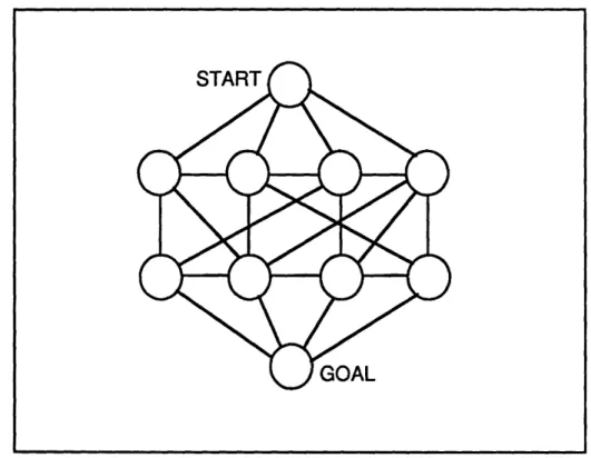
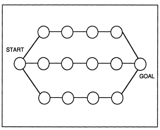
A depth first search would be an effective technique where there are many options at each node, but relatively few nodes in the solution string (see Figure 2-2). It would not, however, be as desirable in a search space with long solution strings and relatively few options at each node (see Figure 2-3). (The reverse situations apply to the breadth first search.)

Figure 2-2. Node space with short solution string

By comparison, A* avoids wasting time searching unproductive areas of node

space by placing emphasis on the most promising directions. This effect is accomplished by using a heuristic cost estimate to identify the best node candidates. The search begins as the start node is expanded. In expanding a node, the possible successor nodes are

Chapter 2. Background

with the actual cost of going from the parent to the child node, A* adds a best guess of the cost to complete a solution from that child node by using information about the vehicle, the environment, and the particular mission.

A* then rank orders the generated (successor) nodes on a memory stack called the OPEN List and places the expanded (parent) node on a separate stack called the CLOSED List. The search is continued by pulling the next node to be expanded from the top of OPEN. The search is terminated when the goal node is pulled from OPEN. The solution string is then generated by backtracking from child to parent, starting with the goal and ending at the start node.

Figure 2-3. Node space with long solution string

During the search, if there are multiple routes to a given node, then as paths (strings) are generated, the information set for a particular node reflects the most efficient

ST

Chapter 2. Background

path to get there. A* has been proven guaranteed optimal over the search space if the heuristic is admissible [11]. A heuristic cost is admissible if the estimate is less than or equal to the actual cost. Aggressive heuristics, which are close to the actual cost, accelerate the search by providing better information about the cost to successfully accomplish the specified maneuver. Such estimates, however, are usually accompanied by higher computational cost.

The A* methodology is demonstrated in a sample problem formulation--the Roadmap Problem, where the object is to get from a start node to a goal node using a network of roads. The heuristic estimate is the air distances between the nodes.

AN EXAMPLE OF AN A* SEARCH: THE ROADMAP PROBLEM

Consider the history of the roads in the Boston area; most of the roads are asphalt versions of what used to be cow trails connecting the various towns in a more or less tangled network. A frequent challenge for the automobile commuter is to find the quickest route from one town to another, which may involve accounting for the presence of an obstacle.

The start node is Wayland. The goal is to get to Lexington before the shot is heard 'round the world. (See Figure 2-4a.) The start node is the first parent node and is the first to be expanded. In expanding a node, its successors are generated. This means that "children" nodes have information tags associated with them that identify their parent node (PATH), the actual cost to go from the parent to the child node (GCOST), and an estimate as

to the cost to complete the journey to the goal from the child node (HCOST). In this problem formulation, GCOST is given by: g(N,N') = actual distance by road between the

Chapter 2. Background

two nodes. (N represents the parent node and N' a child node.) The heuristic estimate,

HCOST, is given by h(N') = the line-of-sight distance (or "as the crowflies ") from the the child node to the Goal.

The search begins by putting the start node (Wayland) on the OPEN stack. The

OPEN stack is a rank-ordered list of candidate nodes for expansion. These nodes are

ordered by their total cost, FCOST: f(N,N')=g(N,N')+h(N'). The start node is the first node to be expanded; in this problem, the generation function simply tells A* to consider the towns geographically adjacent to Wayland: Lincoln, Concord, and Waltham (see Figure 2-4b). A* now places the parent node (Wayland) on the CLOSED stack (the listing of nodes that have been expanded) and generates the children nodes. After computing the actual distances and estimating the air distance between each of the town centers, A* ranks Lincoln, with a total cost (FCOST) of 18, as number one for expansion on the OPEN stack.

While the colonists think that they have found the optimal path to Lexington, unforeseen to them is the sabotage of a bridge by the repressors of religious freedom. Because the bridge is unpassable, it represents an obstacle. As Lincoln is expanded and put on the CLOSED list, the generation of Lexington as a child of Lincoln is penalized because of the presence of this obstacle (see Figure 2-4c). Consequently, while the FCOST for Lexington as a child node of Lincoln would have been 19, it is now 49 because A* has assigned a obstacle penalty of 30 to this route. A* continues with the expansion of Lincoln as Concord and Waltham are generated. Since the costs of these nodes as children of Lincoln exceed the generations from Wayland, these nodes are removed (or pruned) from the OPEN list. Similarly, if a node on CLOSED was found to be an inferior generation it would be removed from the CLOSED list, assigned the new generation information (PATH, GCOST, HCOST, and FCOST) and entered again on the OPEN list. At this point, number one on the OPEN list is Concord.

Chapter 2. Background

The search continues as Concord is expanded (see Figure 2-4d). The children nodes for Concord are Bedford, Lincoln, and Lexington. As previously noted, A* avoids extra effort by pruning duplicate states from both the OPEN and CLOSED lists. In this generation, the new child node, Lincoln from Concord is compared to an earlier node generation (Lincoln from Wayland) and is found inferior. The Lincoln from Concord node is therefore never entered on the OPEN list. After completing the expansion of Concord, A* observes that the FCOST for Lexington as a child node of Concord (as opposed to being a child node of Lincoln) now places Lexington on the top of OPEN. A* then terminates the search as the Goal has been pulled from the top of the OPEN stack.

Observing the final configuration of the planning road map in Figure 2-4d, we note that two possible nodes were not expanded, Bedford and Waltham. Were an exhaustive node search or a Dynamic Programming method used, the computational costs of

expanding these nodes would have been required, unless a degree of optimality was to be sacrificed.

TRAVEL BETWEEN BOSTON AREA TOWNS

Wayland _{Figure 2-4a}

OPEN LIST CLOSED- LIST

w.-ay IJ • I w I I

iwa.ln I's

17

NODE I n L... Co*c" Be"or= Fiaure 2-4d Inglon Waltham

SPATH H T CLOSEP LIST

POoD PATH O H ICOst Noo PATH o

r Canord .12 10 1 ?i

Wal n. Wtayand It II I

itedias Concord 9.

La, ... --- I--

I--

I1

Lare l Waylpnd i ii Ceeana Wapland 0 12 7 SLgbflom L U 17+1 t 0 4N:*2 L V Blo.,rd Figure 2-4c Concord dnglon Waltham

DeEK.LEIf CLOBED LIB

NDE PATH a H FPOOT NOD PATH 0 N FO

Cenoad wed 12 W a- I --

--Wallha Waand 12 10 LI omo Waylnd I 11

"FCOST Include a pena1sy for Mle obstacle

(30). N RcorT OS ] v DTa ysaLunoulrama:~N~*v~n~6cbhlEono-- LEXINGTUNI v

Chapter 3. A*Search

3 A* SEARCH: TRAJECTORY PLANNING WITH

ANOMALIES

The implementation of an optimal search algorithm using the A* search posed two major challenges. The first was the creation of an efficient and meaningful node space; the second was a method of determining the cost of getting from one node to another node. This chapter also characterizes the link between the planner and autopilot, ending with a

summary of the implementation of the various concepts and tools introduced in this investigation of the A* technique.

GRID ASSIGNMENT CONCEPTS

In developing an efficient and meaningful grid, two approaches were investigated reflecting different relative emphasis on two design considerations--the representation of

the full range of options available and the preclusion of nodes that were physically unachievable or redundant. These roughly correspond to the Linear Algebra concepts of the spanning and linear independence of a space, the ideal gridspace corresponding to a basis.

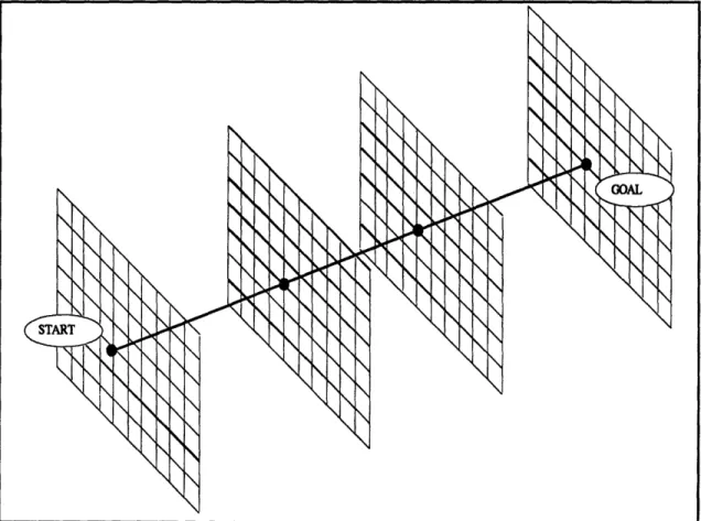
Spatial Grid Assignment: The first concept generated a uniform grid of nodes. A regular lattice structure was constructed to represent a linear discretization of the space surrounding the line of sight between the start and goal nodes. A variation to the concept included nodes "behind" the start node (i.e. in directions opposite from the goal) and "beyond" the goal node to provide options for longer transfers or delays before requiring a jet firing. As a further improvement, node density was varied to provide a finer

distribution of choices in the vicinity of the start, goal, or obstacle locations. In these areas, small changes in trajectory could result in large changes in cost. It therefore made sense to increase the node concentration in these areas.

Chapter 3. A*Search

The motion required by the linear grid (see Figure 3-1) did not, in general, correspond to unforced trajectories. Many velocity changes were made so that the vehicle

would pass through the points represented by this uniform grid, rather than follow the natural trajectories defined by orbital mechanics. The end effect was a trajectory which required trim bums at each node to account for the discontinuities associated with the linear discretization. To reduce the numerous jet cyclings, the grid was altered to surround a nominally optimal two-impulse trajectory, creating a node space with more curvature.

Figure 3-1. Spatial Grid Assignment--a linear discretization of space.

These efforts significantly enhanced A* performance. Even with these

improvements, however, the search occasionally developed trajectories that caused the vehicle to enter an infinite looping trajectory (between three or four nodes), appearing to

Chapter 3. A*Search

mimic cycloid motion. These trajectories were caused in part by the discretized nature of the spatial grid. Rather than producing a travelling-circle solution characterized by the cycloid, the planner, confined to the static spatial grid produced a closed loop trajectory. While cycloid motion specified a node somewhere in between two nodes which the spatial grid provided, the planner was constrained to choose a node which did not corresponded to a coasting trajectory. If the node which turned out to be the lower cost alternative

happened to complete a closed curve, an infinite looping trajectory was created, producing an unuseable solution.

Spatial Grid assignment created a node space which represented the full range of spatial locations available to the planner, at the expense of a severe computational burden. Significant developments using pruning techniques would have been necessary to make the Spatial Grid Assignment concept workable. Further difficulties were encountered when considering the discretization of time. Each node could lie on any of infinitely many actual trajectory arcs, each differing in energy and transfer time. Picking the transfer time from this infinity of possibilities became a substantial task. While we could have picked a suitably small range of times to limit the task, there was no guarantee that the optimal time would be in this range.

Dynamic Grid Assignment: A more efficient method of creating a meaningful grid space uses vehicle dynamics and orbital mechanics to generate candidate nodes in the vehicle's state space (i.e. the six-space reflecting the three translational displacements and velocities) as opposed to the Spatial Grid Assignment approach which represents

displacements only. Starting with the initial conditions on the start node (ov_0 specified), a nominal trajectory is computed using a nominally optimal transfer time (NOMTIM) for a two-impulse solution.

Chapter 3. A*Search

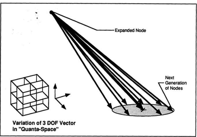
The nominal trajectory determines a velocity required, yR, at the node being expanded for a vehicle to arrive at the goal location in the specified transfer time. A jet select algorithm [12], which models vehicle and actuator dynamics, then computes the quantized firing times and records the specified jets. The quantized firing times are stored in a 3-vector called the quanta vector, q. Each component of the quanta vector is varied, using a 27 point stencil, by a pre-specified percentage (e.g. 20%) so that the individual components are given 20% greater, 20% less, or identical value to the nominal to create the next generation of nodes (see Figure 3-2). Up to twenty-six distinct variations on the nominal quanta vector, g(N') are generated by applying permutations of a weighting vector, for example:

q(N')1 0 0

g(N"') = g(N')

+4

0 .2 0 ]

0

q(N')

0

(N"') = g~(N') +[.2 0 0 ]

0

q(N')2

0

The minimum variation amount in any component is one quanta. Because these vectors represent quantized jet firing intervals, if any component of g(Ni_{) is negative because of the}

variations, that vector is discarded.

In addition to the nominal trajectory and the twenty-six variations, a twenty-eighth option is added corresponding to no firing: g(N(28_{)) = 0. This node allows the vehicle to}

simply coast during consecutive time increments, giving the planner the option of creating no-fire periods where the chase vehicle waits for a more opportune time to execute a burn. As an example, consider the case where the chase and the target vehicles are not in the same orbit plane. It may be beneficial to wait until the chase vehicle is in the plane to execute a burn that reduces the remainder of the rendezvous problem to an in-plane maneuver. Each

Chapter 3. A*Search

of these twenty-eight options represents a different trajectory available to the planner as a follow-on segment from the parent node in building a multi-bum solution.

Figure 3-2. Generation of variations on the nominal trajectory.

To generate these trajectories, the specified impulsive velocity change is applied to the parent node's state vector. Using the state transition matrix, the node is then

propagated forward in time by a set time increment (DELTAT) which is a fraction of the nominal transfer time (NOMTIM) to generate a child node. The new state is then recorded. In total, each node that is expanded generates up to 28 successors including the 26

variations on the nominal trajectory, the no firing option and the nominal trajectory (which will put the vehicle on a coasting trajectory to the goal).

The method is labelled "dynamic" for two reasons. First, it reflects the dynamics of the vehicle. As such, the node pattern or grid space is unique to the vehicle. The

30

Node

Variation of 3 DOF Vector

in "Quanta-Space"

on

Chapter 3. A*Search

significance is that the vehicle can actually achieve the states associated with every node

generated. Second, nodes are generated as the search proceeds. This directly implies that

the grid is an evolving structure and is unique, not only to the vehicle, but to the problem as

well. By contrast to the spatial grid concept, where the node pattern is predetermined and

independent of the problem scenario, the dynamic grid is flexible and responsive to the

specific geometries and constraints of the given situation.

The node pattern using dynamic grid assignment is inherently more efficient as it

generates nodes that are located in the natural trajectories given by orbital mechanics. By

involving the vehicle and actuator dynamics in node generation we implicitly account for

effects such as jet discretization and can easily accommodate vehicle configuration changes

such as failed jets by updating the jet selection data base. Further, since the grid only

includes physically reachable states (in physical and velocity space), we have essentially

pruned the large number of unreachable nodes encountered in the spatial grid assignment.

Although a dense grid that represents all possible control combinations offered by

the vehicle could conceivably have been created, on something with as many redundant

effectors as the space shuttle, far too many nodes would have been generated. If, for

example, at each node the full range of jet combinations (forty-four effectors taken three at

a time) was generated, rather than twenty-eight successors we would have thirteen

thousand. Realizing that some of these possible successors would not produce useful

trajectories, it is clear that a more manageable subset of the full range of combinations (such

as the quanta variation scheme with twenty-eight successors), while not exhaustive, would

be more desirable.

While optimizing the fuel consumption during the planning of the mission is an

important objective, it should not be the overriding focus of a planner. The requirements

Chapter 3. A*Search

for safety and assurance of mission success should take precedence over local optimization of fuel consumption. The goal of this design effort was to arrive at a neighboring optimal controller which could safely avoid significant obstacles that evolve with time such as the malfunctioning satellite which may have erratic movement. In order to attain this capability, the search must be computationally efficient. In pursuit of the real-time capabilities desired, we favor the dynamic grid assignment concept and as sparse a grid as possible. The

obvious counter concern is that sufficient variations are provided to the search for it to develop an. perturbed trajectory that will allow successful circumnavigation of any obstacles encountered. The resolution of these competing concerns should be reflected in the

specification of parameters set by the Maneuver Manager's program logic.

CALCULATING THE COST

The second major development, the method of calculating the cost of node propagation, is a very natural outgrowth of using the jet select algorithm in node

generation.

The A* search algorithm depends on the calculation of two costs, a generation cost,

GCOST (N,N'), and an heuristic cost, HCOST (N'). In both calculations the primary function

is the generation of the velocity required, _yR, which is determined by the two node

locations and a transfer time. In generating GCOST (N,N'), the velocity required at the parent node to arrive at the child node in the specified time increment (DELTAT) is calculated and the velocity change between the coasting velocity at the parent node, yC, and the velocity required, y.R, is passed to the jet select algorithm, which calculates the quanta vector. The quanta required for the velocity change is stored as the generation cost of the child node, N', from the parent node, N: GCOST(N,N')= QUANTA G ( (Y at N) - (YC at N)).

Chapter 3. A*Search

To compute the heuristic cost, HCOST (N'), a similar operation is done where the child node, N', takes the place of the parent node and the goal node takes the place of the child node. In addition to the the cost of the burn at N', we also add the cost of the deceleration burn to null the coasting velocity at the goal node as well. HCOST(N')=

QUANTAH ((XR at N') - (yC at N))+ QUANTAH ((YC at GOAL)). The transfer time is the difference between the nominal time (NOMTIM) and the flight time at N'. If N' is along a lengthy search string the flight time may be equal to or greater than NOMTIM. If this is the case the transfer time to the goal is one DELTAT.

It is important to note that in calculating the heuristic there is an assumption made regarding the admissibility of the estimate. The admissibility requirement is that the heuristic cost must be less than or equal to the actual cost of completion. A more

aggressive heuristic would seek to provide a very close estimate of the actual cost. In this development, the formulation of the HCOST quanta function is not the same as the one used in the GCOST calculation. In order to speed up the computation, we use an ideal jet

implementation rather than invoking the jet select algorithm for the two velocity changes. The effect is to make the heuristic less aggressive. Biasing the estimate in the opposite direction, the possible non-optimality of an immediate two-bum trajectory between the child node and the goal may produce a heuristic cost that is larger than the actual cost. This calls into question the admissibility of the estimate. The heuristic calculates the cost for a two-bum transfer in a specific transfer time. While the transfer time is almost certainly non-optimal, the two-bum trajectory is itself non-optimal in some cases. The effects of the inadmissibility of the heuristic have been noted in some test cases, indeed resulting in the planning of a non-optimal trajectory.

While an admissible heuristic could be easily produced by simply scaling the

existing heuristic, this would decrease the aggressiveness of the heuristic. Alternatively, an 33

Chapter 3. A*Search

exact and optimal solution from each candidate node to the goal could be calculated by a traditional method such as variational calculus, but this would be time consuming and defeat the intent of a real time planner, creation of an efficient algorithm. Instead, noting that the more significant objectives of mission success and vehicle safety are attained by this optimizing planner, the aggressiveness and computational efficiency of using a two-burn trajectory as the heuristic is chosen over possible admissibility with a different estimator.

LINKS TO THE AUTOPILOT

As a part of the APOPS system, the Trajectory Planner sends a waypoint file to a trajectory buffer for the Execution Manager to access. This waypoint file contains three items of information: the waypoint in the form of the chase vehicle's state vector, the time tag associated with the waypoint, and a flag that states whether the waypoint is a forced fire point. As opposed to a reference waypoint which is provided solely for the error

regulation, the forced fire point corresponds to a node contained in the solution string which requires a velocity change.

The Digital Autopilot (DAP) reads the waypoint file using it as a reference path. The DAP functions as a regulator, using the waypoints and the time tags to compare the actual state vector to the planned (reference) trajectory, keeping the vehicle state vector within a pre-specified error bound. While the jet select used in the search algorithm is the

same as used in the DAP, the planned firings are adjusted or augmented to regulate error. Finite quantization of jet impulses, imperfect modelling and disturbances prevent the autopilot from precisely nulling position and rate errors. In order to cause the vehicle to move from one end of the error sphere to another (so that average position is close to the reference), a small perturbation in the requested jet firing is implemented. This causes the

Chapter 3. A*Search

vehicle to limit cycle along the reference trajectory as it moves toward the target. In order that planner-requested firings (which may be on the same order of magnitude as these limit cycle firings) are not ignored, a flag is provided to force a jet firing at those specific

waypoints corresponding to the solution nodes in the search's grid space.

IMPLEMENTATION

As discussed in chapter 2, the dynamics model used in this effort is the linearized Clohessy-Wiltshire equations of motion. This dynamics model accounts for accelerations on bodies due only to the gravitational attraction of a spherical earth. The state transition matrix form of the solution to the Clohessy-Wiltshire equations is used to generate candidate nodes that represent the states in the three translational degrees of freedom and the three associated translational velocities. The search employs the developments discussed earlier in this chapter-- a grid that contains these nodes and a cost function and heuristic estimate on which the A* search algorithm is based. The inputs to the search are

(1) the initial conditions on the vehicle and any obstacles, (2) the terminal conditions on arrival at the goal, (3) a nominal transfer time, (4) the variation factor (which governs the percentage of variation of the quanta vector), and (5) a time constraint on the trajectory.

DETERMINING THE NOMINAL TRAJECTORY

The search starts by computing a nominal trajectory from the start node to the goal node using the two-impulse trajectory associated with the nominal time. The velocity change required at the start node is calculated so that the vehicle's state vector will reflect the velocity required, VR, to achieve the nominal trajectory to the target. The calculation of yR proceeds from the ) matrix, evaluated at the nominal time. If we divide the matrix into

Chapter 3. A*Search

quadrants we can rearrange the equations to compute the velocity needed to pass through a desired node. xl

X1

[

11

0i121

Y0o

_R(0,X1)

=

0 =

)12

Y1

-

)

YR(k~ ,l), then represents the velocity required at the start node (xo,yo,zo) so that a

spacecraft will arrive at the goal state(xl,yl,zl) in the nominal time.

The nominal velocity change required is the difference between the required velocity, yR(2i,ox 1), and the current coasting velocity vector, vc. (In the expansion of the

start node, vc= yo. In expanding subsequent parent nodes, vc corresponds to the velocity at that node, resulting from the previous coasting trajectory.) This velocity change request is then passed to a linear programming algorithm for jet selection, which in this case is

identical to the DAP's jet select algorithm. (The linear programming problem is to solve for x, where w = Ax, such that xi 0> for all xi, and Yfixi is minimized.) The output of the jet

select is a vector of on-times for specified jets.

VARYING THE QUANTA AND GENERATING THE CHILD NODES

As described earlier in this chapter, this vector of quantized firing times, called the quanta vector, is altered by the variation factor (the percentage called for at the initiation of

Chapter 3. A*Search

the program) using the 27 point stencil and the no-firing option. The twenty-eight on-time combinations, u(Ni) are then converted into velocity changes. If A is an acceleration matrix

and u(Ni) is the quanta vector which generates the ith node, the expression for the new parent velocity vector is:

yp(N

A new state vector at the parent node is defined by augmenting the displacement

components of the parent node, rp=[xp,yp,Zp] with the new velocity vector,

yp(Ni)4ip(Ni),yp(Ni),ip(N)]. The new parent vector is propagated using the state transition matrix through one time interval (DELTAT) to arrive at the child node, x(Ni).

(Note: [xp,yp,zp]=[xo,yo,zo] in the start node expansion.)

x(N') y(N') z(N') - (N')

i(N)

Zp

_ gN

This process of creating a parent velocity vector, yp(Ni), and augmenting the displacement vector, rp=[xp,yp,zp], with it to form a new parent vector, occurs for each child node generation. This illustrates the differing natures of the two grid assignment schemes discussed earlier. Nodes created using Dynamic Grid Assignment (the method presented) are actually generated by implementable control effort and lie on natural, unforced

Chapter 3. A*Search

COMPUTING GCOST AND HCOST

There are two components to the total cost, FCOST, which is the index used in

sorting the candidate nodes. The generation cost, GCOST, is the quanta for the desired

velocity change which puts the chase vehicle on a coasting trajectory from the parent to the

child node: GCOST(NN')= QUANTA G [XP -

xC],

The heuristic estimate, HCOST, represents the ideal firing times associated with the two impulsive velocity changes required to put the chase vehicle on a coasting trajectory from the child node to the goal and terminate the maneuver at that point. Given the child node's state vector, x(Ni), computed in the last section, the algorithm then computes the velocity required at the child node:

0- x(Ni)

-[1,

y-R((N'),GOAL) = 012

0

-

y(Ni)

1 0 . z(Ni) J

where the (D sub-matricies are computed with the appropriate terminal time. In this

development, the terminal time is the nominal time (one of the inputs to the planner), unless the time index for the child node is already greater than or equal to the nominal time. If this is the case, the terminal time is extended by one DELTAT beyond the current time. As in the GCOST calculation, the impulsive velocity change required is computed to achieve the specified YR.

The second impulsive velocity change is required to null the chase vehicle's projected terminal velocity at the end of the heuristic coasting trajectory. By propagating the child node's altered state vector (i.e. the child node's displacement vector augmented

Chapter 3. A*Search

with the velocity required, pR(Q(Ni), GOAL)) forward in time, we get the projected terminal state and the chase vehicle's terminal velocity.

XF(N i) yF(N')

zF(N')

iF(N

S21

022

Taking the sum of these two impulsive changes, and dividing by the specific thrust of a single jet, we get an idealized jet firing time.

HCOST=( IX(N) - yR((Ni),GOAL)J y~ - 0 ) / specific thrust

HCOST represents the ideal jet firings where the vehicle's effectors are located exactly along the direction of the velocity change required and have no minimum on-times. (Typically, jets will have a minimum firing time; firing requests which fall below that threshold are not implemented, or implemented by an effector with a different geometry. The Space

Shuttle's threshold of 80 milliseconds is the basis for the quantized bum interval defined earlier in the chapter.)

CHECKING FOR OBSTACLE INTERCEPTION

To check for obstacles that may intercept the trajectory of the chase vehicle, we take an obstacle's state vector and propagate it in time up to the current flight time.

Chapter 3. A*Search

BossT--(t)(t,to)BossT(to)

During the time interval between the parent and child nodes the state vectors of the chase vehicle and the obstacle(s) are propagated in increments of one twentieth of the time increment, DELTAT. The obstacles have been modelled as uniform spheres, so if the magnitude of the difference between the displacement components of the state vectors is smaller than the sum of the chase vehicle and obstacle radii, a collision has been predicted and a penalty is applied to GCOST(NN'). The effect of this penalty is to increase the cost of this node and which causes this candidate to be sorted toward the bottom of the OPEN list. As a possible alternative, future implementations of the algorithm could simply remove the node from the list altogether. In practice, a collision is unacceptable, so carrying this node at the bottom of the OPEN list merely adds to the computational baggage of the search.

SORTING THE NODE AND STORING REQUIRED INFORMATION

Summing the generation and heuristic costs (including any penalty from a collision with an obstacle), we get the total cost, FCOST= GCOST+HCOST. The child node is now sorted on the OPEN list where the node reflecting the least costly alternative at the top of the stack.

Additional information is also stored in reference to the newly generated node. The child node's parent is recorded on PATH (Ni), for use at the termination of the search to recover the solution string. The current flight time is computed by adding the time

increment, DELTAT, to the parent's flight time and the result is stored in FLTnIM (Ni). After

each of the variations, g(Ni), have been used to generate the child nodes, the expansion of the parent node is complete and the parent is placed on CLOSED.

Chapter 3. A*Search

The search continues as the next parent node is pulled off the top of the OPEN stack. Before expanding the next node, the associated flight time is checked against the time constraint, TIMCON. If after adding one DELTAT to the flight time, the time constraint is violated, the parent node is discarded and the search continues with the next node on the

OPEN list. (A time constraint is a typical feature of fuel optimal control problems; if time is

unconstrained or not penalized, solution trajectories often produce a do nothing strategy since it is the lowest cost alternative [13].)

TERMINATING THE SEARCH

The A* search algorithm typically terminates when the goal node is pulled from the OPEN stack. However, because control effort discretization and computational

inaccuracies contribute to produce inherent numerical errors, this application of the search algorithm terminates the search when the candidate parent node is physically located within a sphere that surrounds the goal. The goal sphere in this implementation has a radius of 3 feet.

Following termination of the search, the solution string is generated. Using the PATH list, which contains pointer identifying the parents of each node, the algorithm backtracks beginning with the last node. The solution string is completed when the start node is recovered.

GENERATING THE WAYPOINT FILE

The final task for the planner is the generation of a waypoint file. Beginning with the start node, the solution states, _ss, are propagated in time steps of 60 seconds to generate a reference trajectory for the DAP, Xp:

Chapter 3. A*Search

xwp(t+60) = CQ(t+60,to) ss(to),

iwp(t+120) = O(t+120,to) xss(to), ....

The propagation from the start node continues until the time at which the next state in the solution string is reached. At that point, the next node on the solution string takes the place of the start node and the base time reference for the D matrix is the time index (FLTTIM) associated with that node.

For each of the nodes in the solution string, xss, a flag is set to identify that waypoint as a forced firing point requiring the DAP to implement the best velocity change possible to rectify the vehicle's actual state vector with the reference trajectory. The last waypoint entry is a forced firing to achieve the goal state; the chase vehicle arrives at the origin and nulls its closing velocity.

Chapter 4. Testing

4 TESTING

THE SIMULATION

Four test cases were simulated on the existing Draper Space Systems Simulator to demonstrate the Trajectory Planner's capability to successfully maneuver to an orbiting target while avoiding obstacles. The Space Systems Simulator is a high fidelity simulation of on-orbit vehicular motion. The gravity model used for all of the test cases was a

spherical earth. To demonstrate disturbance accommodation, the J2 gravity term, due to an oblate earth, was used to introduce a disturbance which had not been accounted for in the trajectory planner's dynamics model. The simulator can also account for the environmental effect of gravity gradient torque on vehicle attitude, but does not account for atmospheric effects such as aerodynamic drag. The differential equations of motion in the six degrees of freedom are independently integrated by a fourth-order Runge-Kutta algorithm.

The vehicles used in these simulations are the Space Shuttle (the maneuvering or chase vehicle), the Orbital Maneuvering Vehicle (the obstacle or intercepting vehicle), and the Hubble Space Telescope (the target vehicle). While the attitude dynamics and

orientation can be arbitrary in the simulation, shuttle attitude was held fixed, aligned with the LVLH coordinate frame so that the nose of the shuttle was pointed along the velocity vector.

TESTING DESCRIPTION

In each of the four test cases, the planner started with a nominal transfer time, from which it produced a nominal execution plan. To test the ability of the planner to revise

Chapter 4. Testing

plans to accomplish obstacle avoidance, an intercepting trajectory was computed for the obstacle which would place it directly in the chase vehicle's nominal path. Given the obstacle's trajectory, A* then developed a perturbed trajectory for the pursuer which avoided the obstacle. (See the Appendix for a sample planning history where the planner makes use of information about the obstacle.)

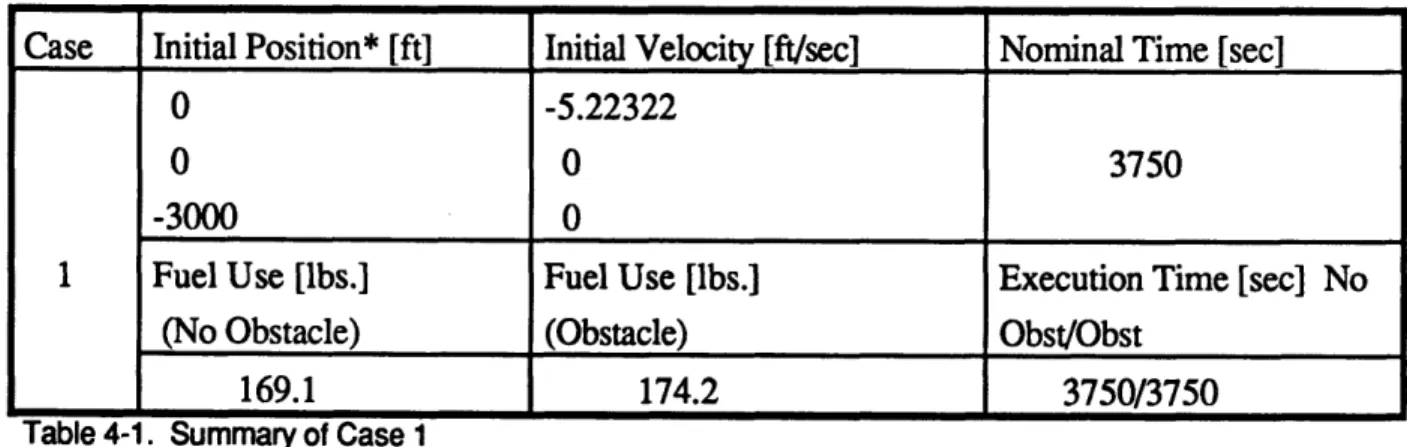
In the problem statement, the initial and terminal states may be assigned arbitrary displacements and velocities. In these cases, the initial states were given velocities corresponding to nearly circular Keplerian orbits and the target state was located at the origin of the LVLH coordinate system. The planner's task is to specify a trajectory for the chase vehicle from the initial offset position to the target, while avoiding any obstacles, meeting a constraint on terminal velocity, and optimizing the solution generated from the

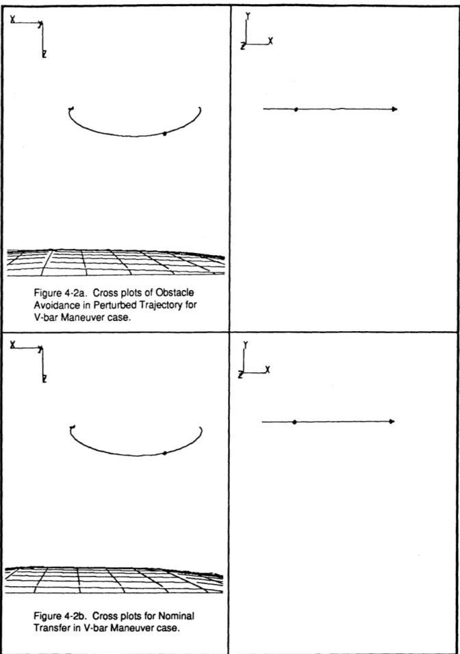
node space. Data is presented reflecting the fuel expenditures associated with the nominal transfers as well as the perturbed trajectories which accomplish obstacle avoidance. Trace plots show the path taken by the chase vehicle during the transfers. A representation of the

obstacle is shown in both the nominal and obstacle runs to demonstrate the collision of the obstacle with a vehicle on a nominal trajectory and the successful avoidance of the

intercepting obstacle on the perturbed trajectory.

A multiple obstacle problem with three intercepting vehicles is also posed to

demonstrate the flexibility of the A* Trajectory planner. An additional comparison with the solution of a simple two-impulse trajectory solver demonstrates the effectiveness of the optimization accomplished by A*. Finally, disturbance accommodation, readily available to the integrated APOPS system, is illustrated by introducing an unplanned disturbance to the waypoint execution on the simulator.