Water quality failures in distribution networks - risk analysis using fuzzy logic and evidential reasoning

Publisher’s version / Version de l'éditeur:

Risk Analysis, 27, October 5, pp. 1381-1394, 2007-10-01

READ THESE TERMS AND CONDITIONS CAREFULLY BEFORE USING THIS WEBSITE. https://nrc-publications.canada.ca/eng/copyright

Vous avez des questions? Nous pouvons vous aider. Pour communiquer directement avec un auteur, consultez la

première page de la revue dans laquelle son article a été publié afin de trouver ses coordonnées. Si vous n’arrivez pas à les repérer, communiquez avec nous à [email protected].

Questions? Contact the NRC Publications Archive team at

[email protected]. If you wish to email the authors directly, please see the first page of the publication for their contact information.

NRC Publications Archive

Archives des publications du CNRC

This publication could be one of several versions: author’s original, accepted manuscript or the publisher’s version. / La version de cette publication peut être l’une des suivantes : la version prépublication de l’auteur, la version acceptée du manuscrit ou la version de l’éditeur.

Access and use of this website and the material on it are subject to the Terms and Conditions set forth at

Water quality failures in distribution networks - risk analysis using fuzzy logic and evidential reasoning

Sadiq, R.; Kleiner, Y.; Rajani, B. B.

https://publications-cnrc.canada.ca/fra/droits

L’accès à ce site Web et l’utilisation de son contenu sont assujettis aux conditions présentées dans le site LISEZ CES CONDITIONS ATTENTIVEMENT AVANT D’UTILISER CE SITE WEB.

NRC Publications Record / Notice d'Archives des publications de CNRC:

https://nrc-publications.canada.ca/eng/view/object/?id=59fddd05-e672-44ef-af2f-87eda44b0a45 https://publications-cnrc.canada.ca/fra/voir/objet/?id=59fddd05-e672-44ef-af2f-87eda44b0a45

http://irc.nrc-cnrc.gc.ca

W a t e r q u a l i t y f a i l u r e s i n d i s t r i b u t i o n

n e t w o r k s – r i s k a n a l y s i s u s i n g f u z z y l o g i c

a n d e v i d e n t i a l r e a s o n i n g

N R C C - 5 0 0 8 3

S a d i q , R . ; K l e i n e r , Y . ; R a j a n i , B .

A version of this document is published in / Une version de ce document se trouve dans: Risk Analysis, v. 27, no. 5, Oct. 2007, pp. 1381-1394

The material in this document is covered by the provisions of the Copyright Act, by Canadian laws, policies, regulations and international agreements. Such provisions serve to identify the information source and, in specific instances, to prohibit reproduction of materials without written permission. For more information visit http://laws.justice.gc.ca/en/showtdm/cs/C-42

Les renseignements dans ce document sont protégés par la Loi sur le droit d'auteur, par les lois, les politiques et les règlements du Canada et des accords internationaux. Ces dispositions permettent d'identifier la source de l'information et, dans certains cas, d'interdire la copie de documents sans permission écrite. Pour obtenir de plus amples renseignements : http://lois.justice.gc.ca/fr/showtdm/cs/C-42

Water quality failures in distribution networks - risk analysis using

fuzzy logic and evidential reasoning

Rehan Sadiq, Yehuda Kleiner, and Balvant Rajani

Buried Utilities Research Urban Infrastructure Program Institute for Research in Construction (IRC)

National Research Council of Canada (NRC), Ottawa, ON, Canada K1A 0R6

Abstract: The evaluation of the risk of water quality failures in a distribution network is a

challenging task given that much of the available data are highly uncertain and vague, and many of the mechanisms are not fully understood. Consequently, a systematic approach is required to handle quantitative-qualitative data as well as means to update existing information when new knowledge and data become available.

Five general pathways (mechanisms) through which a water quality failure can occur in the

distribution network are identified in this paper. These include contaminant intrusion, leaching and corrosion, biofilm formation and microbial regrowth, permeation, and water treatment breakthrough (including disinfection byproducts formation). The proposed methodology is demonstrated using a simplified example for water quality failures in a distribution network. This paper builds upon the previous developments of aggregative risk analysis approach.

Each basic risk item in a hierarchical framework is expressed by a triangular fuzzy number, which is derived from the composition of the likelihood of a failure event and the associated failure consequence. An analytic hierarchy process is used to estimate weights required for grouping non-commensurate risk sources. The evidential reasoning is proposed to incorporate newly arrived data for the updating of existing risk estimates. The exponential ordered weighted averaging operators are used for defuzzification to incorporate attitudinal dimension for risk management. It is

envisaged that the proposed approach could serve as a basis to benchmark acceptable risks in water distribution networks.

Keywords: Fuzzy logic, evidential reasoning, water quality, distribution networks, exponential ordered weighted average operators, and analytic hierarchy process.

____________________________________________________________________________________

INTRODUCTION

Safety of drinking water is a high priority of water purveyors and stakeholders (owners and customers). A typical modern water supply system comprises the water source (groundwater or surface water including the catchment basin), transmission mains, treatment plants and a distribution network, which includes pipes and distribution tanks. While water quality can be compromised at any component, failure at the distribution level can be extremely critical because it is closest to the point of delivery and, with the exception of a rare filtering device at the consumer level, there are virtually no safety barriers before consumption.

Water quality failures

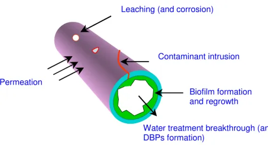
Water quality is generally defined by a collection of upper and lower limits on selected indicators (contaminants) in the water (Maier, 1999), which can be classified into three broad categories: physical, chemical and biological contaminants. The upper and lower limits are often governed by regulations (Swamee and Tyagi, 2000). A water distribution network acts as a complex reactor in which various processes occur simultaneously. The water quality in the distribution network, which is an outcome of these processes, continuously changes both temporally and spatially. A water quality failure event is often defined as an exceedance of one or more water quality indicators from specific regulations, or in the absence of regulations, exceedance of guidelines or self-imposed, customer-driven limits. Water quality failures in distribution networks can generally be classified into the following major categories or pathways (Kleiner, 1998), also described in Figure 1:

• Contaminant intrusion into the distribution network through system components,

• Biofilm formation and regrowth of microorganisms in a distribution network,

• Water treatment breakthrough of bacteria and/ or chemicals, formation of disinfection byproducts (DBPs),

• Leaching of chemicals, release of corrosion byproducts, and

An intrusion of contaminants into the water distribution network can occur through storage tanks (animals, dust-carrying bacteria, infiltration) and pipes. Intrusion through water mains may occur during or after maintenance and repair events, through broken or corroded (pinholes or cracks) pipes and joints/ gaskets, and through cross-connections (Kirmeyer et al., 2001). Whenever the water pressure in a pipe is very low or negative, the risk of contamination through backflow or through leaky pipes increases. This can happen when the pipe is de-pressurized for repair or during transient pressures (e.g., when the hydrant is used for fire extinguishing or water hammer events).

Biofilm is a deposit consisting of microorganisms, microbial products and detritus at the surface of pipes or tanks. Biological regrowth may occur when injured bacteria enter from the treatment plant into the distribution network. Under favorable conditions, such as nutrient supply (e.g., organic carbon) in the water and long residence time, these bacteria can attach themselves to surfaces, rejuvenate and grow in storage tanks and on rough inner surfaces of water mains. The regrowth of microorganisms in the distribution network results in an increased chlorine demand, which has two adverse effects: (a) a reduction in the level of free available chlorine may hinder the network’s ability to contend with local occurrences of contamination (US EPA, 1999), and (b) an increased level of disinfection to satisfy the chlorine demand of biofilm may result in higher concentrations of disinfection byproducts (DBPs).

Internal corrosion of metallic pipes and plumbing devices may increase the concentration of metal compounds in the water. Different metals go through different corrosion processes, but in general low pH water, high dissolved oxygen, high temperature, and high levels of dissolved solids increase corrosion rates. Metals such as lead and cadmium may leach into the water from pipes, causing significant health effects. Secondary metals such as copper (from home plumbing), iron (distribution pipes) and zinc (galvanized pipes) may leach into water causing taste, odor and color (red or rusty water) problems in addition to some minor health-related risks (Kleiner, 1998). Leaching of chemicals into the water supply can often come from the internal lining and coating of pipes (e.g., volatile organic compounds), causing physico-chemical water quality failure with adverse health and aesthetic consequences.

Permeation is a phenomenon in which contaminants (notably hydrocarbons) from polluted site migrate through the walls of plastic pipes. Three stages are observed in permeation: (a) organic chemicals present in the soil partition between the soil and the plastic wall, (b) the chemicals defuse

through the pipe wall, and (c) the chemicals partition between the pipe wall and the water inside the pipe (Kleiner, 1998). In general, the risk of contamination through permeation is relatively small as compared to other mechanisms.

Risk analysis techniques

Commonly, “risk” refers to the joint probabilities of an occurrence of an event and its consequences and “risk analysis” refers to a process of an estimation of the frequency and physical consequences of undesirable events (Ricci et al., 1981). Risk analysis may include a range of techniques from a simple qualitative analysis (e.g., preliminary hazard analysis) to very complex quantitative techniques (e.g., Bayesian networks) for dynamic systems. A brief discussion on some of the risk analysis techniques is provided in this section.

Preliminary hazard analysis (PHA) is a qualitative technique for conducting hazard

assessment in chemical process industries. The PHA can identify systems/ processes, which require further examination to control major hazards (Fullwood and Hall, 1988). Hazard and operability study (HAZOP) is a technique also commonly employed in chemical process industries for estimating safety risk and operability improvements (Sutton, 1992). Failure mode and effects

analysis (FMEA) is commonly used in reliability engineering to analyze potential failure modes in a system and rank them according to their severity. When the FMEA is extended to criticality

analysis, the technique is called failure mode and effects criticality analysis (FMECA) (Chakib et al., 1992).

Tree-based (hierarchical) techniques are also widely used to perform risk analysis. A fault tree is a logical diagram, which shows the relation between system failure, i.e. a specific undesirable event in the system, and failures of the components of the system (Vincoli, 1994). Event tree

analysis (ETA) is a technique to illustrate the sequence of outcomes, which may arise after the occurrence of a selected initial event (Suokas and Rouhiainen, 1993). Cause-consequence analysis (CCA) combines cause analysis (described by fault trees) and consequence analysis (described by event trees).

Techniques for the analysis of dynamic systems can involve methods such as digraph/ fault graph, dynamic ETA, Bayesian networks, or fuzzy cognitive maps. The digraph/ fault graph technique uses the mathematics and language of graph theory, which constructs the risk model by

replacing system elements with AND and OR gates. Bayesian networks (BN) are directed acyclic graphs, in which nodes represent variables and directed arcs describe the conditional dependence relations embedded in the model. Though the conditional probabilities are often difficult to obtain, BNs are considered as one of the most popular dynamic modeling tools (Pearl, 1988). A fuzzy cognitive map (FCM) is an illustrative representation of the complex system uses cause-effect relationships to perform risk analysis (Kosko, 1986). Recently, MacGillivray et al. (2006) provided an excellent review of some of these risk analysis and decision making strategies. This review critically analyzes and reports a wide range of research studies, which use above risk analysis techniques primarily focusing on drinking water supply systems.

The quantification of the risk of contamination in water distribution networks is a difficult task. Water distribution networks comprise many (sometimes thousands of) kilometers of pipes of different ages and various materials, which are subjected to varying operational and environmental conditions. In addition, limited performance and deterioration data are available since pipes are buried structures. Finally, some of the failure processes are not well understood and the diagnosis of contamination is very difficult because there is generally a time lag between the occurrence of failure and the time at which the consequences (e.g., outbreaks) are observed.

Both set theory and probability theory are the classical mathematical frameworks for

characterizing uncertainties. Since the 1960s, a number of generalizations of these frameworks have been developed to formalize different types of uncertainties. Klir (1999) reported that well-justified measures of uncertainties are available not only in the classical set theory and probability theory, but also in the fuzzy set theory (Zadeh, 1965), possibility theory (Dubois and Parade, 1988), and the Dempster–Shafer (D–S) theory (Dempster, 1968; Shafer, 1976). Klir (1995) proposed a

comprehensive general information theory (GIT) to encapsulate these concepts into a single framework and established links among them.

Sadiq et al. (2004) developed a hierarchical (or tree-based) structure that broke down the overall risk of water quality failures in a distribution network into basic risk items. Risk was characterized qualitatively (or linguistically) based on fuzzy techniques combined with an analytic hierarchy process (AHP). This paper builds upon the previous developments and addresses four important aspects of the aggregative risk analysis in distribution networks. These aspects are: (a) Risk fuzzification – mapping of triangular fuzzy numbers of basic risk items to 5-tuple fuzzy risk

set, (b) Risk aggregation – aggregating fuzzy risk for hierarchical structure (c) Risk updating - using evidential reasoning to fuse newly arrived data (or belief) with existing knowledge, and updating risk estimates at any level in the hierarchical structure, and (d) using exponential ordered weighted average (E–OWA) operators for defuzzification to consider the decision-maker’s attitude towards risk (level of optimism) when deriving the final expressions for aggregative risk.

THE PROPOSED FRAMEWORK

In many engineering problems, information about the probabilities of various risk items is vaguely known or assessed. Fuzzy logic provides a language with syntax and semantics to translate qualitative knowledge into numerical reasoning. When conducting risk analysis for complex systems, decision-makers, engineers, managers, regulators and other stakeholders often articulate the risk in terms of linguistic variables like very high, high, very low, low etc. The fuzzy-based techniques are able to deal effectively with such vague and imprecise probabilities for approximate reasoning, which subsequently help the decision-making process.

Triangular fuzzy numbers (TFNs) are often used for representing linguistic variables (Lee, 1996). A more comprehensive description of fuzzy-based techniques is not provided in this paper because of space limitations. Interested readers are encouraged to consult excellent texts on this topic written by Klir and Yuan (1995) and Ross (2004).

(a) Risk fuzzification

Let the likelihood (probability) r of failure be defined by the triangular fuzzy number TFNr

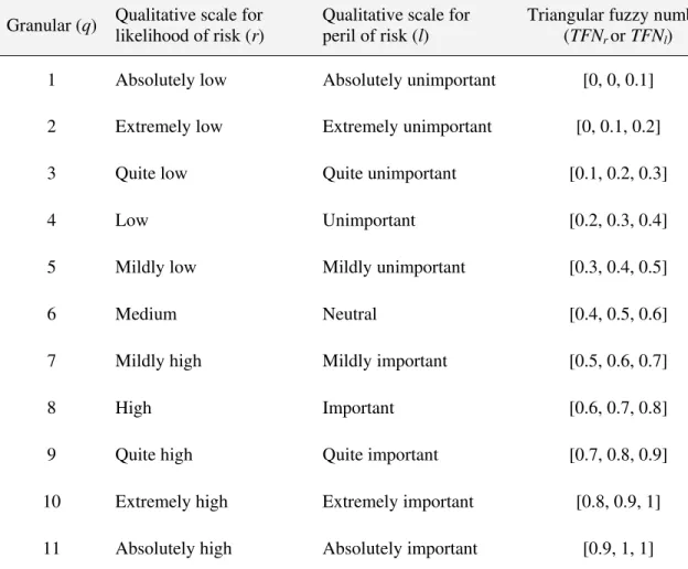
and the consequence (or peril) l of failure be defined by TFNl. Table 1 describes an 11-grade scale

for both r and l. Let failure risk be defined by the 5-grade TFNL, described in Table 2. The

definitions of TFNs can be changed or modified based on expert opinion or on Delphi based surveys.

The risk of failure in the probabilistic realm is the joint probability of occurrence and consequences of failure. When the probabilities of occurrence and failure are assumed to be independent of each other, their joint probability is equal to the product of the respective probabilities. Under the same assumption of independence, the fuzzy risk of failure will be

two TFNs is itself a TFN. Let TFNr be defined by the members (ar, br, cr), and TFNl by (al, bl, cl).

The risk TFNrl for these r and l is calculated by,

x = TFNrl = TFNr × TFNl = (ar * al, br * bl, cr * cl) (1)

For example, if an event has a likelihood r as high [0.6, 0.7, 0.8] and the peril l is

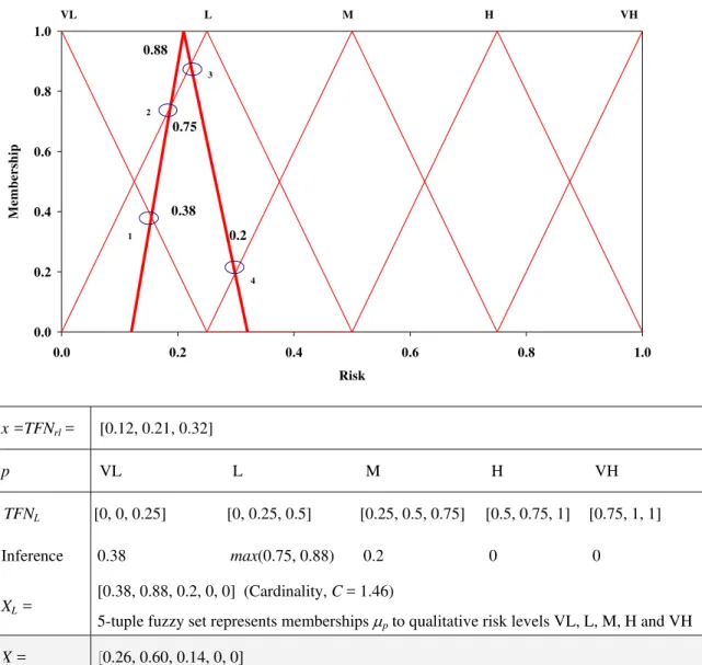
unimportant [0.2, 0.3, 0.4], the corresponding risk x will be a TFNrl [0.12, 0.21, 0.32]. There are 5

steps to convert fuzzy number TFNrl into fuzzy risk X - a normalized 5-tuple fuzzy set. These steps

are also illustrated in Figure 2.

• Map TFNrl over TFNL (p = 5-grades defined over the universe of discourse of risk);

• determine the points where TFNrl intersects each TFNL (Table 2);

• use a maximum (or-type, t-conorm) operator if TFNrl intersects any TFNL at more than one point

(Figure 2);

• establish a set of intersecting points (or the maximum thereof if more than one) that defines a non-normalized 5-tuple fuzzy set, XL, (e.g. in Figure 2, XL is [0.38, 0.88, 0.2, 0, 0], which are the

memberships of XL to the grades very low, low, medium, high and very high risk, respectively);

and

• normalize XL to obtain fuzzy set X, where membership μp of XL is transformed to μpN of X by

dividing each μp by the cardinality C (sum of all memberships in a fuzzy set).

C p n p p p N p μ μ μ μ = ∑ = =1 (2)

In the example of Figure 2, the fuzzy set X is [0.26, 0. 6, 0.14, 0, 0], and can also be expressed as, =_⎢⎣⎡ _⎥⎦⎤ VH H M L VL X 0.26,0.6,0.14, 0 , 0 . (b) Risk aggregation

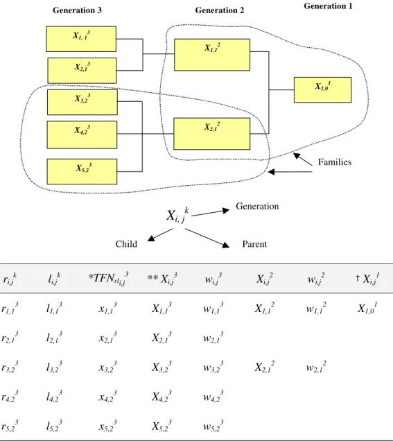
Figure 3 illustrates the basic building blocks of the proposed hierarchical structural model for the risk aggregation. Each risk item is partitioned into its contributory factors, which are also risk items, and each of those can be further partitioned into lower level contributory factors. A unit that consists of a risk factor (“parent”) and its contributory factors (“children”) is called a “family”.

A risk unit with no children is called “basic risk item”, while the term risk item is used for all elements with offspring. The notation used for a risk item is Xi,jk, where i is the ordinal number of

risk item X in the current generation; j is the ordinal number of the parent (in the previous

generation); and k is the generation order of X. The indices i, j, k are used for risk item attributes as well, e.g., in the table of Figure 3, the factors ri,jk and li,jk denote likelihood and peril (respectively)

for the risk item Xi,jk.

Various “inferencing” methods can be used to aggregate fuzzy sets, however in this study, “inferencing” through weighted average is proposed to determine the aggregative risk. The

weighted average inferencing refers to sum-prod fuzzy compositional operator. There are different types of fuzzy composition operators available like max-min (reflects low uncertainty range), sum-prod (reflects high uncertainty range) and mix of both max-min and sum-sum-prod. These compositional operators express the various degrees of and-ness and or-ness in the application of fuzzy sets. Logical operators like max-min are more restrictive than, say, sum-prod and max-prod. For simplicity the weighted average (sum-prod) is used in this study (Sadiq et al., 2003).

A weighting scheme is required when the respective contributions of sibling risk items towards their parent have non-commensurate units. Figure 3 shows a general case where weights are assigned to each risk item. The notation used is wi,jk, which denotes the weight of Xi,jk relative to

its siblings. When the respective contributions of sibling risk items towards their parent have commensurate units, then all the siblings have equal weights, wi,jk , which means that they can be

ignored altogether. Saaty (2001) described in detail the analytic hierarchy process to derive weights. These weights are normalized to a sum of unity, such that in any generation (k), for n siblings with parent j, a set of weights can be written as,

[

]

The process of evaluating aggregative risk in a “family” with an aggregative structure is described using the family (Figure 3) of X2,12 (parent) and X3,23, X4,23, X5,23(children) as an example.

For each of the sibling risk items, the likelihood r and peril l are assigned from the 11-grade scaling system (Table 1). TFNrl(x) is the product of two fuzzy numbers TFNr and TFNl (Equation 1), which

is then mapped over TFNL to obtain the 5-tuple fuzzy set XL (a non-normalized fuzzy set for risk).

contribution of each of the siblings towards their parent. For ease of manipulation these 5-tuple sets can be arranged in a fuzzy assessment matrix, which is a 3 × 5 matrix F(Xi,23). The AHP is then

applied, weights w3,23, w4,23, and w5,23are evaluated and arranged into a 3-member vector. The

aggregative risk (or parent) of the three siblings is the cross product of weights vector and the assessment matrix, yielding a 5-tuple fuzzy set X2,12,

[

]

[

]

where μpN (p = 1, 2,…, 5) are the membership values of the aggregated risk with respect to the

5-grade risk scale.

It should be noted that the process of evaluating r and l and mapping the product risk onto the 5-grade risk scale is necessary only for basic risk items, i.e. those risk items, which do not have children. All subsequent risk aggregations from one generation to the next are determined by only applying equation (4) using the appropriate relative weights. Consequently it is useful to use notation that distinguishes between basic and non-basic risk items. In the remainder of this paper, the notation for a basic risk item will include an apostrophe at the generation index, i.e., if item X4,23

is a basic risk item, it will be denoted by X4,23’.

(c) Risk updating using evidential reasoning (D–S rule of combination)

In classical Bayesian inference, the sum of probabilities of any set A and its complement, p(A) + p(¬A) = 1. This implies that knowledge about A can be used to derive a belief about its complement. For example, let Θ = {A, B, C}, be a frame of discernment (also called a universe of discourse meaning all possible outcomes), and let the evidence p(A) = a. According to equal

noninformative priors (Laplace Principle of Insufficient Reason), then p(B) = p(C) = 0.5(1 - a), i.e., the probability of the complement of A will be equally distributed in subsets B or C.

In contrast to the above, Dempster–Shafer (D–S) theory is based on the premise that missing evidence (or lack of knowledge, or ignorance) about ¬A does not justify an assumption about probabilities of B and C (Alim, 1988). The D–S theory can be interpreted as a generalization of probability theory, where probabilities are assigned to subsets as opposed to mutually exclusive singletons. For example, let the universal set {L, M, H} contain three basic elements. The frame of discernment Θ comprise all combinations of the basic elements in the universal set, in our example,

the 8 subsets of Θ are φ, {L}, {M}, {H}, {L, M}, {L, H}, {M, H}, and {L, M, H}. The subset {L, M} means {L} or {M}. Consequently, the subset {L, M, H} represents a complete ignorant situation (i.e., we do not know which will be the outcome, it can be any of L, M or H). It can be shown that Θ comprises 2n subsets where n is number of basic elements.

The D–S theory defines a basic probability assignment (bpa is denoted by m). Let evidence A be a subset of Θ. The bpa m(A) is defined over the interval [0, 1]. The bpa of a null set m(φ) = 0. The complement of A is always attributed to the complete ignorance, i.e., subset Θ. For example, let evidence A = {{L}, {L, M}} so that m(A)L = 0.6 and m(A)L,M = 0.2, then m(A) = 0.8 and m(A)Θ =1 0.8. For a given basic probability assignment m, every non-ignorant subset A (i.e., m(A) ≠ 0) is called focal element, e.g., in the example above, m(A)L and m(A)L,M are focal elements.

The D–S rule of combination defines how to combine evidence obtained from two or more sources. It strictly emphasizes agreements between multiple sources and ignores all conflicting evidence through normalization. A strict conjunctive operation (and-type or intersection type operator) using a “product” is used to combine the evidences. For example, if B and C are two sources of information, the D–S rule of combination establishes the joint bpa m1-2(A) from the aggregation of bpas m1(B) and m2(C),

φ ≠ − ∑ = ∩ = − when A K ) C ( m ) B ( m ) A ( m B C A 1 2 1 2 1 ; m1-2 (φ) = 0; (5) where K m(B)m (C) C B 1 2 ∑ = = ∩ φ

K is the degree of conflict between two bodies of evidence. It can be shown that the denominator (1-K) in equation (5) is a normalization factor, which always brings the sum of all m1-2(A) values to unity. The above equations can be rewritten as,

∑ ∑ = ≠ ∩ = ∩ − φ C B A C B ) C ( m ) B ( m ) C ( m ) B ( m ) A ( m 2 1 2 1 2 1 (6)

Zadeh (1984) identified a serious shortcoming in the D–S rule of combination due to the use of strict conjunctive operator (product). Sentz and Ferson (2002) have provided an excellent review of various techniques to overcome this discrepancy. Recently, Yager (2004) proposed the use of

disjunctive operators (or-type operator, denoted by ⊕), according to which, equation (6) can be modified as,

( ) ( )

[

]

[

]

A disjunctive logic using “max” operator can be used in equation (7). The approach described above implicitly assumes that all sources of information are equally credible. Yager (2004) suggested a credibility transformation function, which discounts evidence with a credibility factor (α) and distributes the remaining evidence (1-α) equally among n elements.

n ) A ( m ) A ( m _α = ⋅α +1−α (8)

For example, assume that the evidence obtained from two different sources for risk item X1,12 are represented by fuzzy sets m1(X1,12) = [0.5, 0.5, 0, 0, 0] and m2(X1,12) = [0, 0.6, 0.4, 0, 0]. Assume further that the corresponding credibility factors are α1 = 1 and α2 = 0.5, respectively. The bodies of evidence are adjusted and the D–S rule of combination is used to obtain the fuzzy set m1-2(X1,12) = [0.33, 0.33, 0.2, 0.07, 0.07]. In the hierarchical structure described earlier, D–S updating can be done at any level of the hierarchy when new evidence is available, however, it is expected that D–S updating will be done mainly at the level of basic risk items. This process is thus used to combine the new information with prior information.

(d) Risk management (using defuzzification)

In the first generation of the aggregative structure (i.e., the head of the pyramid), the final aggregative risk is a fuzzy set that can be defuzzified to provide a single (crisp) measure of the risk, using one of the several defuzzification techniques described in Chen and Hwang (1992). Lee (1996) proposed a simple defuzzification technique as follows,

Defuzzified risk = L_P⋅X_1,01 (9)

which means that the defuzzified risk is calculated as a dot product of vector LP and the fuzzy

number X1,01, where LP (given in Table 2) is the 5-tuple vector representing centroid values of p

uncertainties and subjectivity in the use of any defuzzification technique. An attitudinal dimension can be introduced in the defuzzification of risk to alleviate (or at least have control over) this issue.

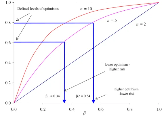
In the proposed framework the ordered weighted operators (OWA) as described by Yager (1988) is selected as the method to consider the attitude of the decision-maker in defuzzifying the final risk value. The OWA method was used for applications in decision-making (Engemann et al., 1996), expert systems (Kacprzyk, 1990), and fuzzy systems (Yager and Filev, 1994). A number of approaches have been suggested to obtain OWA weights (Yager, 1993). O’ Hagan (1988), for example, calculated the vector of the OWA weights for a predefined orness (level of optimism) by maximizing the entropy of the OWA weights using linear programming. Another (simpler) way of obtaining OWA weights involves the using of exponential OWA (E–OWA) operators, which represent a simple relationship between the orness and a parameter β (Filev and Yager, 1998). The E–OWA weights are defined as follows:

w1 = β; w2 = β (1 - β); … wn-1 = β (1 - β) n - 2 and wn = (1 - β) n – 1 ; 0 ≤ β ≤ 1 (10) where n is the granularity of fuzzy risk. Once the weights wp (p = 1, 2, …, n)are determined, the

crisp value of the fuzzy risk can be calculated by

Defuzzified risk = N (11) p n p p w μ ∑ =1

where μpN are the normalized membership values of the fuzzy risk to the risk levels, which are

arranged in a decreasing order of importance (i.e., VH, H, M, L, VL). Parameter β is determined based on the decision-maker’s chosen optimism level or orness. The orness of an E-OWA operator takes on a value between zero (pessimistic) and unity (optimistic) and is related to parameter β as follows

(

)

Figure 4 illustrates some characteristic curves of orness versus β for selected levels of granularity, as calculated using equations (10) and (12). In summary, the steps to estimate risk for a given level of optimism are:

• calculate β using equations (10) and (12) or read the value of β from the characteristic curve (Figure 4) with the appropriate number of granulars;

• determine weights using equation (10); and

• determine crisp risk estimates using equation (11).

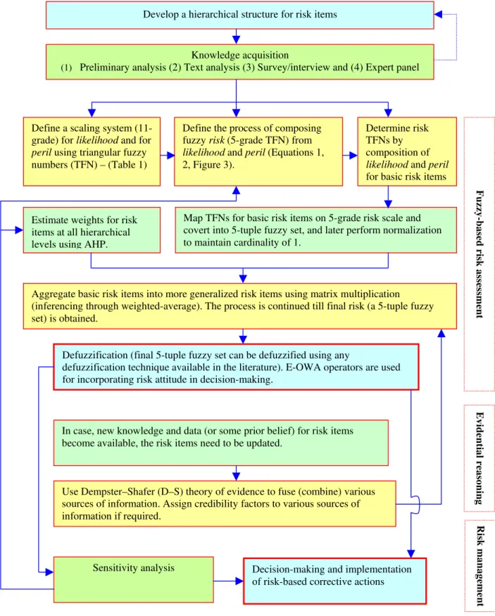
The risk estimates of alternative strategies at a desired level of optimism can be associated to cost-benefit analysis. The more optimistic the attitude, the higher the willingness to take risks and the lower the cost of risk mitigation. Conversely, lower optimism results in a conservative approach, which involves higher costs. Figure 5 provides a block diagram that illustrates the proposed

framework.

WATER QUALITY FAILURE IN DISTRIBUTION NETWORKS

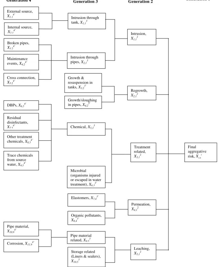
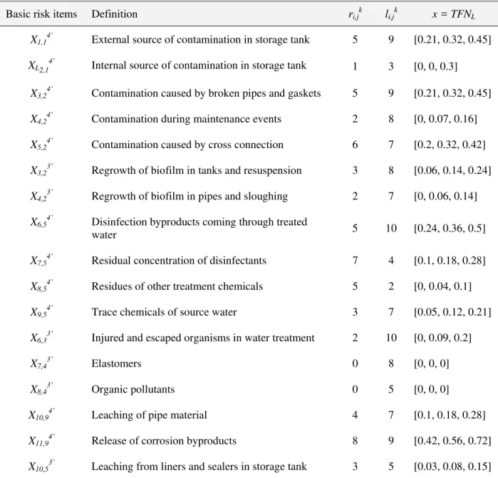
Figure 6 shows a simplified hierarchical structure for water quality failure. A detailed discussion on each type of water quality failure can be found in Sadiq et al. (2004). This structure is used to demonstrate the aggregative risk framework introduced in the previous section. Table 3 lists 17 basic risk items for the proposed structure. These basic risk items are positioned in the fourth and the third generations of the hierarchical structure, and are grouped into the third and the second generations (respectively) risk attributes, which in turn are grouped further up the hierarchy. The weight matrices wi,jk for each set of siblings were developed using the AHP technique as discussed

earlier.

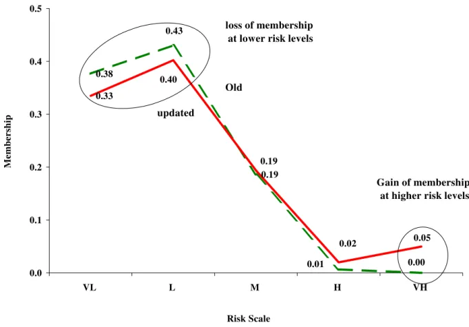
The process of basic risk evaluation and subsequent risk aggregation through all the generations were performed as described in the previous section. The final aggregated risk (first generation) was obtained

⎭ ⎬ ⎫ ⎩ ⎨ ⎧ = VH H M L VL

X_1,01 0.38,0.43,0.19,0.01, 0 and is plotted in Figure 7. The final

defuzzified aggregative risk was determined for two levels of orness (optimism) 0.6 and 0.8 (Figure 4). The crisp (defuzzified) risk estimates varied between 0.14 and 0.06 for low and high optimistic attitudes, respectively.

In the context discussed here, the D-S updating is demonstrated by reassessing risk based on available new evidence on microbial contamination. This evidence could consist of information such as an increase in off-the-shelf sales of gastrointestinal medication or additional cases reported

at local clinics/pharmacies. The new evidence m2(X6,33’) was expressed as [0, 0, 0.2, 0.8, 0], with a

credibility (α2) of 1. The old evidence m1(X6,33’) was a 5-tuple fuzzy set [0.58, 0.42, 0, 0, 0] which

was assigned a credibility (α1) of 0.8 with respect to the new evidence. The D–S rule of

combination was used to update this risk item and the value of m1-2(X6,33’) changed to [0.26, 0.21,

0.05, 0.1, 0.37]. The aggregative risk analysis was repeated to obtain a final aggregative risk X1,01 =

[0.33, 0.4, 0.19, 0.02, 0.05]. After defuzzification, the crisp risk estimate changed from 0.14 to 0.15 for the low optimistic attitude level and from 0.06 to 0.09 for the high optimistic attitude level. The results of pre- and post-update possibility mass functions are compared in Figure 7.

SUMMARY AND CONCLUSIONS

Water quality in the distribution network is a complex issue, for which available data are scarce and often highly uncertain, imprecise and vague. In addition, there is a high spatial and temporal variability in water quality may occur, and many of the controlling processes are not currently well understood. A comprehensive framework of risk analysis was proposed for water quality failures in the distribution network. The advantages of the framework are:

• It enables the synthesis of both quantitative and qualitative information into a single framework; • it can explicitly consider and propagate uncertainties, for which probability distributions are not

known;

• it is modular and scalable; and new knowledge and information can be accommodated at any stage and in any form. For example, vulnerability to terrorist acts (safety related risk), hydraulic failure, financial risk etc. can be part of this framework;

• it has ability update information based on newly arrived evidence;

• more data results in less uncertainty, which when propagated through the hierarchical structure, can result in reduced aggregative risk. The proposed approach can help pinpoint (identify) those areas where more data would yield the highest benefits;

• it can be used for cost-benefit analysis to facilitate efficient budget allocation and prioritize attention to those areas which have the most adverse impact on total water distribution network risk; and

• it is easily programmable for a computer application and can become a risk analysis tool for a water distribution network.

The limitations of the proposed method are:

• It may be sensitive to the selection of aggregation operators. Different mathematical operators can be used for different segments of the model and trial and error approach can be used to avoid exaggeration and/or eclipsing. Exaggeration occurs when all basic risk items are of relatively low risk, yet the final aggregative risk comes out unacceptably high. Eclipsing occurs when one or more of the basic risk items are of relatively high risk, yet the estimated

aggregative risk comes out as unacceptably low.

• This framework supports both qualitative and quantitative data. Some data may be supported by rigorous observations, while other data may be based on beliefs that are loosely supported by anecdotal-information. These two types of data should have different weights in the aggregation process. The hierarchical structure in its current form does not address this need to distinguish between data obtained from sources with different reliabilities.

The structure presented in this paper is but a simplified demonstration of the approach. A comprehensive structure would require a major effort, including the collaboration of several experts with knowledge in several disciplines.

In the model development stages, the final aggregative risk value is expected to have limited meaning for the acceptability level of the risk to the general public. It is envisaged that as the

proposed hierarchical structure is developed, risk items are populated and subsequently improved upon (using newly obtained data/evidence), the developers and the guardians of the water

distribution networks will gain insight into acceptable risk levels as they are manifested in the final fuzzy and/ or defuzzified risk values. In the longer term, this approach could serve as a basis to benchmark acceptable risks in water distribution networks. A collaborative research project titled “Effect of aging water mains on water quality in the distribution systems” by American Water Works Association Research Foundation (AwwaRF) and National Research Council Canada (NRC) is dealing with this issue. The result of this research project will be disseminated in coming years.

REFERENCES

Alim, S. 1988. Application of Dempster–Shafer theory for interpretation of seismic parameters, ASCE Journal of Structural Engineering, 114(9): 2070-2084.

Chakib, K-Z., Alfred Z.K. and Fleming, P.V. 1992. A smart failure mode and effect analysis package, Proceedings Annual Reliability and Maintainability Symposium, pp. 414-421.

Chen, S.J., and Hwang, C.L. 1992. Fuzzy multiple attribute decision-making, Springer-Verlag, NY. Dempster, A. 1968. A generalization of Bayesian inference, Journal of Royal Statistical Society,

Series B 30: 205-247.

Dubois, F., and Parade, H. 1988. Possibility theory: an approach to computerized processing of uncertainty, Plenum Press, NY.

Engemann, K.J., Miller, H.E., and Yager, R.R. 1996. Decision making with belief structure: an application in risk management, International Journal of Uncertainty, Fuzziness and Knowledge-Based Systems, 4: 1-6.

Filev, D.P. and Yager, R.R. 1998. On the issue of obtaining OWA operator weights, Fuzzy Sets and Systems, 94: 157-169.

Fullwood, R.R., and Hall, R.E. 1988. Probabilistic risk assessment in the nuclear power industry, 1st Ed. Pergamon Press.

Kacprzy, J. 1990. Inductive learning from considerably erroneous examples with a specificity based stopping rule, Proceedings of International Conference on Fuzzy Logic and Neural Networks, Izuka, Japan, p. 819.

Kirmeyer, G.J., Friedman, M., Martel, K., and Howie, D. 2001. Pathogen intrusion into distribution system, AwwaRF, Denver, CO, USA.

Kleiner, Y. 1998. Risk factors in water distribution systems, British Columbia Water and Waste Association 26th Annual Conference, Whistler, B.C., Canada.

Klir, G.J., and Yuan, B. 1995. Fuzzy sets and fuzzy logic - theory and applications, Prentice- Hall, Inc., Englewood Cliffs, NJ, USA.

Klir, J.G. 1995. Principles of uncertainty: what are they? why do we need them?, Fuzzy Sets and Systems, 74: 15-31.

Klir, J.G. 1999. On fuzzy set interpretation of possibility theory, Fuzzy Sets and Systems, 108: 263-273.

Kosko, B. 1986. Fuzzy cognitive maps, International Journal of Man-Machine Studies, 24: 65-75. Lee, H.-M. 1996. Applying fuzzy set theory to evaluate the rate of aggregative risk in software

development, Fuzzy Sets and Systems, 79: 323-336.

MacGillivray, B.H., Hamilton, P.D., Strutt, J.E., and Pollard, S.J.T. 2006. Risk analysis strategies in the water utility sector: an inventory of applications for better and more credible decision

making, Critical Reviews in Environmental Science and Technology, 36(2): 85-139. Maier, S.H. 1999. Modeling water quality for water distribution systems, Ph.D. thesis, Brunel

O’ Hagan, M. 1988. Aggregating template rule antecedents in real-time expert systems with fuzzy set logic, Proceedings 22nd Annual IEEE Asilomar Conference on Signals, Systems and Computers, Pacific Grove, CA, pp. 681-689.

Pearl, J. 1988. Probabilistic reasoning in expert systems, San Mateo, CA: Morgan Kaufmann. Ricci, P.F., Sagen, L.A., and Whipple, C.G. 1981. Technological risk assessment series E: Applied

Series No.81, NATO Asi Series, Erice (Italy), ISBN 90-247-2961-0.

Ross, T. 2004. Fuzzy logic with engineering applications, 2nd Edition, John Wiley & Sons, NY. Saaty, T.L. 2001. How to make a decision? Chapter 1, Models, methods, concepts and applications

of the analytic hierarchy process, (Ed.) Saaty, T.L., and Vargas, L.G., Kluwer International Series.

Sadiq, R., Kleiner, Y., and Rajani, B.B. 2003. Forensics of water quality failure in distribution system - a conceptual framework, Journal of Indian Water Works Association, 35(4): 267-278. Sadiq, R., Kleiner, Y., and Rajani, B.B. 2004. Aggregative risk analysis for water quality failure in distribution networks, AQUA - Journal of Water Supply: Research & Technology, 53(4): 241-261.

Sentz, K. and Ferson, S. 2002. Combination of evidence in Dempster-Shafer theory, SAND 2002-0835.

Shafer, G. 1976. A mathematical theory of evidence, Princeton University Press, Princeton, N.J. Suokas, J. and Rouhiainen, V. 1993. Quality management of safety and risk analysis, Elsevier

Science Publishers.

Sutton, I.S. 1992. Process reliability and risk management, 1st Ed. Van Nostrand Reinhold, 1992. Swamee, P.K., and Tyagi, A. 2000. Describing water quality with aggregate index, ASCE Journal

of Environmental Engineering, 126(5): 451-455.

US EPA 1999. Microbial and disinfection byproduct rules – simultaneous compliance guidance manual, United States Environmental Protection Agency, EPA 815-R-99-015.

Vincoli, J.W. 1994. Basic guide to accident investigation and loss control, Van Nostrand Reinhold. Yager, R.R. 1988. On ordered weighted averagng aggregation operators in multi-criteria decision

making, IEEE Transactions on Systems, Man and Cybernatics, 18: 183-190. Yager, R.R. 1993. Families of OWA operators, Fuzzy Sets and Systems, 59: 125-148.

Yager, R.R. 2004. On the determination of strength of belief for decision support under uncertainty – Part II: fusing strengths of belief, Fuzzy Sets and Systems, 142: 129-142.

Yager, R.R. and Filev, D.P. 1994. Parameterized "andlike" and "orlike" OWA operators, International Journal of General Systems, 22: 297-316.

Zadeh, L.A. 1965. Fuzzy sets, Information and Control, 8: 338-353.

Zadeh, L.A. 1984. Review of books: A mathematical theory of evidence, The AI Magazine, 5(3): 81-83.

Permeation

Contaminant intrusion Leaching (and corrosion)

Biofilm formation and regrowth

Water treatment breakthrough (and DBPs formation)

0.0 0.2 0.4 0.6 0.8 1.0 0.0 0.2 0.4 0.6 0.8 1.0 Risk Membership 2 3 1 4 VL L M H VH 0.38 0.75 0.88 0.2 x =TFNrl = [0.12, 0.21, 0.32] p VL L M H VH TFNL [0, 0, 0.25] [0, 0.25, 0.5] [0.25, 0.5, 0.75] [0.5, 0.75, 1] [0.75, 1, 1] Inference 0.38 max(0.75, 0.88) 0.2 0 0 XL = [0.38, 0.88, 0.2, 0, 0] (Cardinality, C = 1.46)

5-tuple fuzzy set represents memberships μp to qualitative risk levels VL, L, M, H and VH

X = [0.26, 0.60, 0.14, 0, 0]

Parent Child

Generation 3 Generation 2 Generation 1

X1, 1 3 X2,13 X3,2 3 X4,23 X5,2 3 X2,1 2 X1,0 1 X1,1 2 Families

X

ri,jk li,jk *TFNrli,j3 ** Xi,j3 wi,j3 Xi,j2 wi,j2 † Xi,j1

r1,13 l1,13 x1,13 X1,13 w1,13 X1,12 w1,12 X1,01

r2,13 l2,13 x2,13 X2,13 w2,13

r3,23 l3,23 x3,23 X3,23 w3,23 X2,12 w2,12

r4,23 l4,23 x4,23 X4,23 w4,23

r5,23 l5,23 x5,23 X5,23 w5,23

*the risk TFNL; ** normalized 5-tuple fuzzy set for risk; † for parent of generation 1, and j = 0

0.0 0.2 0.4 0.6 0.8 1.0 0.0 0.2 0.4 0.6 0.8 1.0 β Orness (degree of optimism) n = 2 n = 5 n = 10 β1 = 0.34 β2 = 0.54 Defined levels of optimisms

lower optimism - higher risk

higher optimism -lower risk

Figure 4. Characteristic curves for representing functional relationships between orness and parameter β to determine E-OWA and crisp risk estimates

Evidenti

al reasoning

Develop a hierarchical structure for risk items

Knowledge acquisition

(1) Preliminary analysis (2) Text analysis (3) Survey/interview and (4) Expert panel

Define a scaling system (11-grade) for likelihood and for peril using triangular fuzzy numbers (TFN) – (Table 1)

Define the process of composing fuzzy risk (5-grade TFN) from likelihood and peril (Equations 1, 2, Figure 3).

Estimate weights for risk items at all hierarchical levels using AHP.

Determine risk TFNs by composition of likelihood and peril for basic risk items

Map TFNs for basic risk items on 5-grade risk scale and covert into 5-tuple fuzzy set, and later perform normalization to maintain cardinality of 1.

Aggregate basic risk items into more generalized risk items using matrix multiplication (inferencing through weighted-average). The process is continued till final risk (a 5-tuple fuzzy set) is obtained.

Defuzzification (final 5-tuple fuzzy set can be defuzzified using any

defuzzification technique available in the literature). E-OWA operators are used for incorporating risk attitude in decision-making.

In case, new knowledge and data (or some prior belief) for risk items become available, the risk items need to be updated.

Use Dempster–Shafer (D–S) theory of evidence to fuse (combine) various sources of information. Assign credibility factors to various sources of information if required.

Sensitivity analysis Decision-making and implementation of risk-based corrective actions

Fuzzy-based r isk asse ssment Risk m a nage ment

Generation 4 _{Generation 3 Generation 2} Generation 1 External source, X1,14’ Internal source, X2,14’ Broken pipes, X3,24’ Maintenance events, X4,24’ Cross connection, X5,24’ Growth & resuspension in tanks, X3,23’ Intrusion through pipes, X2,13 Growth/sloughing in pipes, X4,23’ DBPs, X6,54’ Residual disinfectants, X7,54’ Chemical, X5,33 Other treatment chemicals, X8,54’ Trace chemicals from source water, X9,54’ Microbial (organisms injured or escaped in water treatment), X6,33’ Final aggregative risk, X1,0 1 Intrusion, X1,12 Treatment related, X3,12 Elastomers, X7,43’ Organic pollutants, X8,43’ Regrowth, X2,12 Permeation, X4,12 Pipe material, X10,94’ Corrosion, X11,94’ Intrusion through tank, X1,13 Pipe material related, X9,53 Storage related (Liners & sealers), X10,5

3

Leaching, X5,12

0.38 0.19 0.33 0.01 0.00 0.43 0.05 0.40 0.02 0.19 0.0 0.1 0.2 0.3 0.4 0.5 VL L M H VH Risk Scale Membership Old updated loss of membership at lower risk levels

Gain of membership at higher risk levels

Table 1. Linguistic definitions of grades (granulars) using TFNs for likelihood and peril*

Granular (q) Qualitative scale for likelihood of risk (r)

Qualitative scale for peril of risk (l)

Triangular fuzzy number (TFNr or TFNl)

1 Absolutely low Absolutely unimportant [0, 0, 0.1]

2 Extremely low Extremely unimportant [0, 0.1, 0.2]

3 Quite low Quite unimportant [0.1, 0.2, 0.3]

4 Low Unimportant [0.2, 0.3, 0.4]

5 Mildly low Mildly unimportant [0.3, 0.4, 0.5]

6 Medium Neutral [0.4, 0.5, 0.6]

7 Mildly high Mildly important [0.5, 0.6, 0.7]

8 High Important [0.6, 0.7, 0.8]

9 Quite high Quite important [0.7, 0.8, 0.9]

10 Extremely high Extremely important [0.8, 0.9, 1]

11 Absolutely high Absolutely important [0.9, 1, 1]

* For absolute zero and one, “none” and “certain” qualitative scale can be used, respectively. The TFNs for these qualitative scale are (0, 0, 0) and (1, 1, 1), respectively for both likelihood and peril.

Table 2. Linguistic definitions of grades (granulars) using TFNs for risk

Granulars (p)

Qualitative scale for risk level (L)*

Triangular fuzzy number (TFNL) Centroid (LP) 1 Very low [0, 0, 0.25] 0.08 2 Low [0, 0.25, 0.5] 0.25 3 Medium [0.25, 0.5, 0.75] 0.5 4 High [0.5, 0.75, 1] 0.75 5 Very high [0.75, 1, 1] 0.92

* For absolute zero and one, “none” and “certain” qualitative scale can be used, respectively. The TFNs for these qualitative scale are (0, 0, 0) and (1, 1, 1), respectively for both likelihood and peril.

Table 3. Complete data set for basic risk items for the evaluation of final aggregative risk

Basic risk items Definition ri,jk li,jk x = TFNL

X1,14’ External source of contamination in storage tank 5 9 [0.21, 0.32, 0.45]

X_L2,14’ Internal source of contamination in storage tank 1 3 [0, 0, 0.3] X3,24’ Contamination caused by broken pipes and gaskets 5 9 [0.21, 0.32, 0.45]

X4,24’ Contamination during maintenance events 2 8 [0, 0.07, 0.16]

X5,24’ Contamination caused by cross connection 6 7 [0.2, 0.32, 0.42]

X3,23’ Regrowth of biofilm in tanks and resuspension 3 8 [0.06, 0.14, 0.24]

X4,23’ Regrowth of biofilm in pipes and sloughing 2 7 [0, 0.06, 0.14]

X6,54’ Disinfection byproducts coming through treated

water 5 10 [0.24, 0.36, 0.5]

X7,54’ Residual concentration of disinfectants 7 4 [0.1, 0.18, 0.28]

X8,54’ Residues of other treatment chemicals 5 2 [0, 0.04, 0.1]

X9,54’ Trace chemicals of source water 3 7 [0.05, 0.12, 0.21]

X6,33’ Injured and escaped organisms in water treatment 2 10 [0, 0.09, 0.2]

X7,43’ Elastomers 0 8 [0, 0, 0]

X8,43’ Organic pollutants 0 5 [0, 0, 0]

X10,94’ Leaching of pipe material 4 7 [0.1, 0.18, 0.28]

X11,94’ Release of corrosion byproducts 8 9 [0.42, 0.56, 0.72]