Measurement of the Electric Charge of the Top Quark in $\boldsymbol{t\bar{t}}$ Events

arXiv:1407.4837v2 [hep-ex] 25 Sep 2014

V.M. Abazov,31_{B. Abbott,}67 _{B.S. Acharya,}25 _{M. Adams,}46 _{T. Adams,}44 _{J.P. Agnew,}41 _{G.D. Alexeev,}31 G. Alkhazov,35 _{A. Alton}a_,56 _{A. Askew,}44 _{S. Atkins,}54 _{K. Augsten,}7 _{C. Avila,}5 _{F. Badaud,}10 _{L. Bagby,}45 B. Baldin,45 _{D.V. Bandurin,}73_{S. Banerjee,}25 _{E. Barberis,}55 _{P. Baringer,}53_{J.F. Bartlett,}45 _{U. Bassler,}15 V. Bazterra,46 _{A. Bean,}53_{M. Begalli,}2 _{L. Bellantoni,}45 _{S.B. Beri,}23_{G. Bernardi,}14_{R. Bernhard,}19 _{I. Bertram,}39 M. Besan¸con,15 _{R. Beuselinck,}40 _{P.C. Bhat,}45 _{S. Bhatia,}58 _{V. Bhatnagar,}23 _{G. Blazey,}47 _{S. Blessing,}44_{K. Bloom,}59

A. Boehnlein,45 _{D. Boline,}64 _{E.E. Boos,}33 _{G. Borissov,}39_{M. Borysova}l_,38 _{A. Brandt,}70 _{O. Brandt,}20 _{R. Brock,}57 A. Bross,45 _{D. Brown,}14 _{X.B. Bu,}45 _{M. Buehler,}45_{V. Buescher,}21_{V. Bunichev,}33 _{S. Burdin}b_,39 _{C.P. Buszello,}37

E. Camacho-P´erez,28 _{B.C.K. Casey,}45 _{H. Castilla-Valdez,}28 _{S. Caughron,}57 _{S. Chakrabarti,}64 _{K.M. Chan,}51 A. Chandra,72 _{E. Chapon,}15_{G. Chen,}53 _{S.W. Cho,}27 _{S. Choi,}27 _{B. Choudhary,}24 _{S. Cihangir,}45 _{D. Claes,}59 J. Clutter,53 _{M. Cooke}k_,45 _{W.E. Cooper,}45 _{M. Corcoran,}72 _{F. Couderc,}15 _{M.-C. Cousinou,}12 _{D. Cutts,}69 A. Das,42 _{G. Davies,}40 _{S.J. de Jong,}29, 30 _{E. De La Cruz-Burelo,}28 _{F. D´eliot,}15 _{R. Demina,}63 _{D. Denisov,}45

S.P. Denisov,34 _{S. Desai,}45 _{C. Deterre}c_,20 _{K. DeVaughan,}59 _{H.T. Diehl,}45 _{M. Diesburg,}45 _{P.F. Ding,}41 A. Dominguez,59 _{A. Dubey,}24 _{L.V. Dudko,}33 _{A. Duperrin,}12 _{S. Dutt,}23 _{M. Eads,}47 _{D. Edmunds,}57 J. Ellison,43_{V.D. Elvira,}45 _{Y. Enari,}14_{H. Evans,}49 _{V.N. Evdokimov,}34_{A. Faur´e,}15 _{L. Feng,}47 _{T. Ferbel,}63 F. Fiedler,21 _{F. Filthaut,}29, 30 _{W. Fisher,}57 _{H.E. Fisk,}45 _{M. Fortner,}47 _{H. Fox,}39 _{S. Fuess,}45 _{P.H. Garbincius,}45

A. Garcia-Bellido,63_{J.A. Garc´ıa-Gonz´alez,}28 _{V. Gavrilov,}32 _{W. Geng,}12, 57 _{C.E. Gerber,}46 _{Y. Gershtein,}60 G. Ginther,45, 63 _{O. Gogota,}38_{G. Golovanov,}31 _{P.D. Grannis,}64 _{S. Greder,}16 _{H. Greenlee,}45 _{G. Grenier,}17 Ph. Gris,10_{J.-F. Grivaz,}13 _{A. Grohsjean}c_,15_{S. Gr¨unendahl,}45_{M.W. Gr¨unewald,}26 _{T. Guillemin,}13_{G. Gutierrez,}45

P. Gutierrez,67 _{J. Haley,}68 _{L. Han,}4 _{K. Harder,}41_{A. Harel,}63 _{J.M. Hauptman,}52 _{J. Hays,}40 _{T. Head,}41 T. Hebbeker,18 _{D. Hedin,}47 _{H. Hegab,}68 _{A.P. Heinson,}43 _{U. Heintz,}69 _{C. Hensel,}1 _{I. Heredia-De La Cruz}d_,28 K. Herner,45 _{G. Hesketh}f_,41_{M.D. Hildreth,}51 _{R. Hirosky,}73_{T. Hoang,}44_{J.D. Hobbs,}64 _{B. Hoeneisen,}9 _{J. Hogan,}72

M. Hohlfeld,21 _{J.L. Holzbauer,}58 _{I. Howley,}70 _{Z. Hubacek,}7, 15 _{V. Hynek,}7 _{I. Iashvili,}62 _{Y. Ilchenko,}71 R. Illingworth,45_{A.S. Ito,}45 _{S. Jabeen}m_,45 _{M. Jaffr´e,}13_{A. Jayasinghe,}67_{M.S. Jeong,}27 _{R. Jesik,}40_{P. Jiang,}4 K. Johns,42 _{E. Johnson,}57 _{M. Johnson,}45_{A. Jonckheere,}45 _{P. Jonsson,}40 _{J. Joshi,}43 _{A.W. Jung,}45_{A. Juste,}36

E. Kajfasz,12 _{D. Karmanov,}33_{I. Katsanos,}59_{R. Kehoe,}71 _{S. Kermiche,}12 _{N. Khalatyan,}45 _{A. Khanov,}68 A. Kharchilava,62 _{Y.N. Kharzheev,}31 _{I. Kiselevich,}32_{J.M. Kohli,}23 _{A.V. Kozelov,}34 _{J. Kraus,}58 _{A. Kumar,}62 A. Kupco,8 _{T. Kurˇca,}17 _{V.A. Kuzmin,}33_{S. Lammers,}49 _{P. Lebrun,}17 _{H.S. Lee,}27 _{S.W. Lee,}52_{W.M. Lee,}45 _{X. Lei,}42

J. Lellouch,14 _{D. Li,}14_{H. Li,}73_{L. Li,}43 _{Q.Z. Li,}45 _{J.K. Lim,}27 _{D. Lincoln,}45 _{J. Linnemann,}57 _{V.V. Lipaev,}34 R. Lipton,45 _{H. Liu,}71 _{Y. Liu,}4 _{A. Lobodenko,}35 _{M. Lokajicek,}8 _{R. Lopes de Sa,}64 _{R. Luna-Garcia}g_,28 A.L. Lyon,45_{A.K.A. Maciel,}1 _{R. Madar,}19 _{R. Maga˜na-Villalba,}28_{S. Malik,}59_{V.L. Malyshev,}31 _{J. Mansour,}20

J. Mart´ınez-Ortega,28 _{R. McCarthy,}64 _{C.L. McGivern,}41 _{M.M. Meijer,}29, 30 _{A. Melnitchouk,}45 _{D. Menezes,}47 P.G. Mercadante,3_{M. Merkin,}33_{A. Meyer,}18_{J. Meyer}i_,20 _{F. Miconi,}16_{N.K. Mondal,}25 _{M. Mulhearn,}73 _{E. Nagy,}12

M. Narain,69 _{R. Nayyar,}42 _{H.A. Neal,}56 _{J.P. Negret,}5 _{P. Neustroev,}35 _{H.T. Nguyen,}73 _{T. Nunnemann,}22 J. Orduna,72 _{N. Osman,}12 _{J. Osta,}51 _{A. Pal,}70 _{N. Parashar,}50 _{V. Parihar,}69 _{S.K. Park,}27_{R. Partridge}e_,69 N. Parua,49_{A. Patwa}j_,65 _{B. Penning,}45 _{M. Perfilov,}33 _{Y. Peters,}41 _{K. Petridis,}41_{G. Petrillo,}63 _{P. P´etroff,}13

M.-A. Pleier,65 _{V.M. Podstavkov,}45 _{A.V. Popov,}34 _{M. Prewitt,}72_{D. Price,}41 _{N. Prokopenko,}34 _{J. Qian,}56 A. Quadt,20 _{B. Quinn,}58 _{P.N. Ratoff,}39 _{I. Razumov,}34 _{I. Ripp-Baudot,}16_{F. Rizatdinova,}68 _{M. Rominsky,}45

A. Ross,39_{C. Royon,}15_{P. Rubinov,}45 _{R. Ruchti,}51 _{G. Sajot,}11 _{A. S´anchez-Hern´andez,}28 _{M.P. Sanders,}22 A.S. Santosh_,1 _{G. Savage,}45 _{M. Savitskyi,}38_{L. Sawyer,}54_{T. Scanlon,}40 _{R.D. Schamberger,}64 _{Y. Scheglov,}35 H. Schellman,48 _{C. Schwanenberger,}41_{R. Schwienhorst,}57 _{J. Sekaric,}53 _{H. Severini,}67 _{E. Shabalina,}20 _{V. Shary,}15

S. Shaw,57 _{A.A. Shchukin,}34 _{V. Simak,}7 _{P. Skubic,}67 _{P. Slattery,}63 _{D. Smirnov,}51 _{G.R. Snow,}59 _{J. Snow,}66 S. Snyder,65 _{S. S¨oldner-Rembold,}41_{L. Sonnenschein,}18_{K. Soustruznik,}6 _{J. Stark,}11 _{D.A. Stoyanova,}34_{M. Strauss,}67

L. Suter,41 _{P. Svoisky,}67 _{M. Titov,}15 _{V.V. Tokmenin,}31 _{Y.-T. Tsai,}63_{D. Tsybychev,}64_{B. Tuchming,}15 _{C. Tully,}61 L. Uvarov,35 _{S. Uvarov,}35 _{S. Uzunyan,}47 _{R. Van Kooten,}49 _{W.M. van Leeuwen,}29 _{N. Varelas,}46 _{E.W. Varnes,}42 I.A. Vasilyev,34_{A.Y. Verkheev,}31 _{L.S. Vertogradov,}31_{M. Verzocchi,}45 _{M. Vesterinen,}41 _{D. Vilanova,}15 _{P. Vokac,}7

H.D. Wahl,44 _{M.H.L.S. Wang,}45 _{J. Warchol,}51 _{G. Watts,}74 _{M. Wayne,}51 _{J. Weichert,}21 _{L. Welty-Rieger,}48 M.R.J. Williams,49 _{G.W. Wilson,}53 _{M. Wobisch,}54 _{D.R. Wood,}55 _{T.R. Wyatt,}41 _{Y. Xie,}45 _{R. Yamada,}45 S. Yang,4 _{T. Yasuda,}45 _{Y.A. Yatsunenko,}31 _{W. Ye,}64 _{Z. Ye,}45 _{H. Yin,}45 _{K. Yip,}65 _{S.W. Youn,}45 _{J.M. Yu,}56

J. Zennamo,62 _{T.G. Zhao,}41 _{B. Zhou,}56 _{J. Zhu,}56 _{M. Zielinski,}63 _{D. Zieminska,}49 _{and L. Zivkovic}14 (The D0 Collaboration∗₎

2_{Universidade do Estado do Rio de Janeiro, Rio de Janeiro, Brazil} 3_{Universidade Federal do ABC, Santo Andr´e, Brazil}

4_{University of Science and Technology of China, Hefei, People’s Republic of China} 5_{Universidad de los Andes, Bogot´a, Colombia}

6_{Charles University, Faculty of Mathematics and Physics,}

Center for Particle Physics, Prague, Czech Republic

7_{Czech Technical University in Prague, Prague, Czech Republic}

8_{Institute of Physics, Academy of Sciences of the Czech Republic, Prague, Czech Republic} 9_{Universidad San Francisco de Quito, Quito, Ecuador}

10_{LPC, Universit´e Blaise Pascal, CNRS/IN2P3, Clermont, France} 11_{LPSC, Universit´e Joseph Fourier Grenoble 1, CNRS/IN2P3,}

Institut National Polytechnique de Grenoble, Grenoble, France

12_{CPPM, Aix-Marseille Universit´e, CNRS/IN2P3, Marseille, France} 13_{LAL, Universit´e Paris-Sud, CNRS/IN2P3, Orsay, France} 14_{LPNHE, Universit´es Paris VI and VII, CNRS/IN2P3, Paris, France}

15_{CEA, Irfu, SPP, Saclay, France}

16_{IPHC, Universit´e de Strasbourg, CNRS/IN2P3, Strasbourg, France}

17_{IPNL, Universit´e Lyon 1, CNRS/IN2P3, Villeurbanne, France and Universit´e de Lyon, Lyon, France} 18_{III. Physikalisches Institut A, RWTH Aachen University, Aachen, Germany}

19_{Physikalisches Institut, Universit¨at Freiburg, Freiburg, Germany}

20_{II. Physikalisches Institut, Georg-August-Universit¨at G¨ottingen, G¨ottingen, Germany} 21_{Institut f¨ur Physik, Universit¨at Mainz, Mainz, Germany}

22_{Ludwig-Maximilians-Universit¨at M¨unchen, M¨unchen, Germany} 23_{Panjab University, Chandigarh, India}

24_{Delhi University, Delhi, India}

25_{Tata Institute of Fundamental Research, Mumbai, India} 26_{University College Dublin, Dublin, Ireland}

27_{Korea Detector Laboratory, Korea University, Seoul, Korea} 28_{CINVESTAV, Mexico City, Mexico}

29_{Nikhef, Science Park, Amsterdam, the Netherlands} 30_{Radboud University Nijmegen, Nijmegen, the Netherlands}

31_{Joint Institute for Nuclear Research, Dubna, Russia} 32_{Institute for Theoretical and Experimental Physics, Moscow, Russia}

33_{Moscow State University, Moscow, Russia} 34_{Institute for High Energy Physics, Protvino, Russia} 35_{Petersburg Nuclear Physics Institute, St. Petersburg, Russia}

36_{Instituci´o Catalana de Recerca i Estudis Avan¸cats (ICREA) and Institut de F´ısica d’Altes Energies (IFAE), Barcelona, Spain} 37_{Uppsala University, Uppsala, Sweden}

38_{Taras Shevchenko National University of Kyiv, Kiev, Ukraine} 39_{Lancaster University, Lancaster LA1 4YB, United Kingdom} 40_{Imperial College London, London SW7 2AZ, United Kingdom} 41_{The University of Manchester, Manchester M13 9PL, United Kingdom}

42_{University of Arizona, Tucson, Arizona 85721, USA} 43_{University of California Riverside, Riverside, California 92521, USA}

44_{Florida State University, Tallahassee, Florida 32306, USA} 45_{Fermi National Accelerator Laboratory, Batavia, Illinois 60510, USA}

46_{University of Illinois at Chicago, Chicago, Illinois 60607, USA} 47_{Northern Illinois University, DeKalb, Illinois 60115, USA}

48_{Northwestern University, Evanston, Illinois 60208, USA} 49_{Indiana University, Bloomington, Indiana 47405, USA} 50_{Purdue University Calumet, Hammond, Indiana 46323, USA} 51_{University of Notre Dame, Notre Dame, Indiana 46556, USA}

52_{Iowa State University, Ames, Iowa 50011, USA} 53_{University of Kansas, Lawrence, Kansas 66045, USA} 54_{Louisiana Tech University, Ruston, Louisiana 71272, USA} 55_{Northeastern University, Boston, Massachusetts 02115, USA}

56_{University of Michigan, Ann Arbor, Michigan 48109, USA} 57_{Michigan State University, East Lansing, Michigan 48824, USA}

58_{University of Mississippi, University, Mississippi 38677, USA} 59_{University of Nebraska, Lincoln, Nebraska 68588, USA} 60_{Rutgers University, Piscataway, New Jersey 08855, USA} 61_{Princeton University, Princeton, New Jersey 08544, USA} 62_{State University of New York, Buffalo, New York 14260, USA}

64_{State University of New York, Stony Brook, New York 11794, USA} 65_{Brookhaven National Laboratory, Upton, New York 11973, USA}

66_{Langston University, Langston, Oklahoma 73050, USA} 67_{University of Oklahoma, Norman, Oklahoma 73019, USA} 68_{Oklahoma State University, Stillwater, Oklahoma 74078, USA}

69_{Brown University, Providence, Rhode Island 02912, USA} 70_{University of Texas, Arlington, Texas 76019, USA} 71_{Southern Methodist University, Dallas, Texas 75275, USA}

72_{Rice University, Houston, Texas 77005, USA} 73_{University of Virginia, Charlottesville, Virginia 22904, USA}

74_{University of Washington, Seattle, Washington 98195, USA}

(Dated: July 18, 2014)

We present a measurement of the electric charge of top quarks using t¯t events produced in p¯p collisions at the Tevatron. The analysis is based on fully reconstructed t¯t pairs in lepton+jets final states. Using data corresponding to 5.3 fb−1_{of integrated luminosity, we exclude the hypothesis that}

the top quark has a charge of Q = −4/3 e at a significance greater than 5 standard deviations. We also place an upper limit of 0.46 on the fraction of such quarks that can be present in an admixture with the standard model top quarks (Q = +2/3 e) at a 95% confidence level.

PACS numbers: 14.65.Ha, 13.85.Rm, 14.80.-j

The top quark (t), discovered in p¯p collisions at the Tevatron in 1995 [1], fits within the standard model (SM) of particle physics as the companion of the b quark in a weak-isospin doublet with an electric charge of Q = +2/3 e. t¯t pairs via the strong interaction is the domi-nant production mode of top quarks at hadron colliders. In the SM, the top quark decays ≈ 99.9% of the time to a W boson and a b quark, i.e., t(+2/3 e) → W+_{b and} its charge conjugate. However, beyond the SM (BSM) a new quark with a charge of Q = −4/3 e could con-tribute to the same final state with the corresponding decay of qBSM(−4/3 e) → W−b and its charge conju-gate [2][3]. This qBSMis the down-type component of an exotic right-handed doublet with its companion quark having a charge of Q = −1/3 e [2]. The measured kine-matic distributions of t¯t events, in particular, the t¯t mass spectrum, are consistent with the SM [4]. This type of BSM quark would therefore be likely to appear in an ad-mixture with SM top quarks in the t¯t final state, and evade detection unless the charge of the top quarks is measured explicitly.

Under an assumption that, except for the electric charge, all other properties of the BSM quark are iden-tical to those of the SM top quark, experimental limits

∗_{with visitors from} a_{Augustana College, Sioux Falls, SD, USA,} b_{The University of Liverpool, Liverpool, UK,}c_{DESY, Hamburg,}

Germany, d_{Universidad Michoacana de San Nicolas de Hidalgo,}

Morelia, Mexicoe_{SLAC, Menlo Park, CA, USA,}f_University

Col-lege London, London, UK,g_{Centro de Investigacion en}

Computa-cion - IPN, Mexico City, Mexico,h_{Universidade Estadual Paulista,}

S˜ao Paulo, Brazil, i_{Karlsruher Institut f¨ur Technologie (KIT)}

-Steinbuch Centre for Computing (SCC), D-76128 Karlsruhe, Ger-many,j_{Office of Science, U.S. Department of Energy, Washington,}

D.C. 20585, USA,k_{American Association for the Advancement of}

Science, Washington, D.C. 20005, USA, l_{Kiev Institute for}

Nu-clear Research, Kiev, Ukraine andm_{University of Maryland,}

Col-lege Park, Maryland 20742, USA.

have been placed on the BSM nature of the top quark in p¯p collisions at √s = 1.96 TeV by the D0 and CDF collaborations [5, 6], at 92% and 99% confidence levels, respectively. A stringent exclusion has been reported by the ATLAS collaboration in pp collisions at√s = 7 TeV with a significance of more than 8 standard deviations (SD) [7]. In this paper, we discriminate between the SM top quark and the BSM quark under the above assump-tion, using data accumulated with the D0 detector in p¯p collisions at√s=1.96 TeV corresponding to an integrated luminosity of 5.3 fb−1_{. A kinematic fit to the t¯t final} state [8] is used to associate the b jets with the W candi-dates and the charge of the b jets is determined through a jet charge algorithm [9]. We then extend the analysis to examine the additional possibility that the two types of quarks can contribute in an admixture to the top and antitop quarks of the t¯t final state and place a stringent limit on the possible fraction of BSM quarks in the data. The D0 detector [10] has a central tracking system, consisting of a silicon microstrip tracker and a central fiber tracker, both located within a 1.9 T superconduct-ing solenoidal magnet, optimized for tracksuperconduct-ing and ver-texing at pseudorapidities |η| < 3 and |η| < 2.5, re-spectively [11]. Central and forward preshower detec-tors are positioned just outside of the superconducting coil. A liquid-argon and uranium calorimeter has a cen-tral section covering pseudorapidities up to |η| ≈ 1.1, and two end sections that extend coverage to |η| ≈ 4.2, with all three housed in separate cryostats [12]. An outer muon system for |η| < 2 consists of a layer of track-ing detectors and scintillation trigger counters in front of 1.8 T iron toroids, followed by two similar layers after the toroids [13].

We use the lepton+jets final states of t¯t candidate events, where one W boson decays leptonically (W → ℓνℓ with ℓ denoting an electron (e) or a muon (µ)) and the other into two light-flavor quarks (W → q′_{q). The final¯} state is therefore characterized by one isolated charged

lepton of large transverse momentum relative to the beam axis (pT), four jets generally originating from the q′_{, ¯q, b and ¯b quarks, and a significant imbalance in} trans-verse momentum (6ET) resulting from the undetectable neutrino.

The event selection, object identification, and event simulation of signal and background follow the proce-dures described in Ref. [14]. The primary interaction vertex (PV) from a p¯p collision must be reconstructed within 60 cm of the detector center. Electrons are re-quired to have pT > 20 GeV and |η| < 1.1, and muons are required to have pT > 20 GeV and |η| < 2.0. Electrons and muons from leptonic-tau decays (W → τντ → ℓνℓντ) are included in the analysis. Jets are defined using an it-erative cone algorithm [15] with a radius R = 0.5 in (η, φ) space, where φ is the azimuthal angle. We select events with four or more jets with pT > 20 GeV and |η| < 2.5, at least two of which are required to be identified (tagged) as b jets through a neural network (NN) discriminant at a threshold for which the tagging efficiency for b jets is ≈ 55% and the misidentification rate for light-flavor jets is ≈ 2% [16]. The 6ET is required to be greater than 20 and 25 GeV in the e+jets and µ+jets events, respectively. The production of t¯t pairs is simulated using the alpgen _{Monte Carlo (MC) generator [17] with a top} quark mass of 172.5 GeV. We use the pythia [18] pro-gram for parton evolution and geant [19] for simulating the D0 detector. The dominant background process is W +jets production. Several additional sources of back-ground are also considered. We simulate W/Z+jets, di-boson (W W, W Z, and ZZ), and single top quark pro-ductions using alpgen, pythia, and comphep [20], re-spectively. The cross section for each background is nor-malized to next-to-leading-order predictions. The contri-bution from multijet background is estimated from data using the “matrix method” [21].

The assignment of reconstructed objects to the prod-ucts from t¯t decay is achieved through a constrained kinematic fit [8], which, for each possible assignment, minimizes a χ2 _{function using the kinematic} informa-tion of the reconstructed objects assuming the t¯t hy-pothesis for the final state objects. As constraints for the fit, we use the conservation of energy and momen-tum and the masses of the W boson and the top quark, mW = 80.4 GeV and mt= 172.5 GeV, respectively. The b-tagged jets are assumed to be jets originating from b quarks. We utilize the 6ET and the mass constraint on the leptonically decaying W boson to infer the momen-tum of the neutrino. The assignment with the lowest χ2 is used to reconstruct the t¯t decay chain. The b jet that is paired with the W boson that decays into two leptons or two quarks in the t¯t event reconstruction is referred to, respectively, as bℓ or bh. The efficiency of correct assignment for bℓ and bh is ≈ 70%.

The charge of the lepton, Qℓ, determines the charge of the leptonically decaying W boson and consequently the opposite charge is assumed for the W boson that decays to q′_{q. The charge of the quark initiating a jet is esti-¯}

mated from the reconstructed jet charge, Qj, using the method proposed in Ref. [9]. The charge of the bℓand bh is denoted as Qℓ

band Qhb. We combine the charges of each W boson and its associated b jet to compute the charge of the top quark Qℓ

t= |Qℓ+ Qℓb| for the top quark whose W boson decays leptonically, or Qh

t = |−Qℓ+Qhb| for the top quark whose W boson decays into quarks. Using the modulus provides two quantities with the same distribu-tions and thus a statistical benefit from merging them. The values of the b-jet charges Qℓ,h_b are computed from a jet-charge algorithm Qj = (ΣiQi· (pT i)0.5)/(Σi(pT i)0.5), where i runs over all reconstructed tracks within the jet with the requirements that each track has (i) a distance of closest approach within 0.2 cm relative to the PV and pT > 0.5 GeV, and (ii) angular distance with respect to the jet axis ∆R(track, jet) ≡ p(∆η)2_{+ (∆φ)}2 _{< 0.5,} with (iii) at least two tracks satisfying the above require-ments. These track criteria and the exponent of 0.5 are the results of an optimization of the algorithm using sim-ulated t¯t events. Events with both bℓ and bh passing these additional tracking requirements are considered for further analysis. The corresponding efficiency is greater than 0.99. Table I summarizes the sample composition and event yields, following the application of all selection criteria and reconstruction of the charge of the top quark.

TABLE I: Sample composition and event yields following the implementation of all final selections. The quoted uncer-tainties include the statistical and systematic components. The “Dilepton t¯t” process represents t¯t events where both W bosons decaying leptonically and “Other” includes the di-boson and multijet processes. The cross section σt¯t= 7.24 pb

is used for t¯t events [22].

Process Expected events

t¯t 263.1+ 17.9 − 18.7 Dilepton t¯t 9.4+ 0.6_{− 0.7} W + jets 12.7 ± 2.1 Z + jets 1.4 ± 0.5 Single top 3.0 ± 0.4 Other 0.6 ± 1.3 Total expectation 290.2+ 18.1 − 18.8 Observed 286

The reconstruction of the jet charge is studied using a “tag-and-probe” method in an inclusive two-jet (dijet) data sample [23] enriched in b¯b events, referred to as the “tight dijet (TD) sample”. The TD sample consists of events with: (i) exactly two jets, each b tagged, with pT > 20 GeV and |η| < 2.5; (ii) the ∆φ between the two jets of > 3.0 radians; and (iii) one jet (referred to as the “tag jet”) containing a muon (referred to as the “tagging muon”) with pT > 4 GeV and ∆R(µ, jet) < 0.5. We refer to the other jet in the dijet event as the “probe jet”.

The TD sample contains a small fraction of c¯c and light parton dijet events. The contribution from light partons is considered negligible since a MC study finds the

b-tagging efficiency for a light parton jet to be a factor of 20 smaller than for a c jet. The fraction of c¯c events in the TD sample is estimated using the pT of the tagging muon relative to the axis of the tag jet (prel

T ). Muons originating from b-quark decays tend to have larger values in the prel T spectrum than those from c-quark decays. We fit the prel

T distribution in data with the distributions from b¯b and c¯c events simulated using pythia and find that the fraction of c¯c events in the TD sample is xc= 0.093 ± 0.009 (stat). The tagging muon in a dijet event is used to infer the charge of the quark initiating the tag jet and con-sequently to determine whether the probe jet is initi-ated by a quark or an antiquark. However, the tag-ging muon can originate from either a direct decay of a B hadron or “charge-flipping” processes such as cas-cade decays of B hadrons, e.g., b → c → ℓ, or neutral B meson mixings. In the charge-flipping processes, the charge of the tagging muon can be opposite to that ex-pected, and therefore mistag the probe jet. We simulate the charge-flipping processes using Z → b¯b (MC) events generated with the pythia program, and find that a frac-tion xf = 0.352 ± 0.008 (stat) of the tagging muons have a charge opposite to that of the initial b quarks [24]. This value is verified by examining the charge correlation be-tween muons in a subset of the TD data sample where an additional muon, having the same quality as the tagging muon, is required in the probe jet.

The performance of the jet-charge algorithm depends on the kinematic properties of the jet, mainly due to a dependence of the tracking efficiency on pT and |η|. The kinematics of the dijet samples used to extract the jet-charge distributions differ from those of t¯t events, whose jet charges we wish to model. To account for the dif-ferences in the performance arising from these kinematic differences, we first re-weight the t¯t MC events to get the same jet pT and |η| spectra as observed in the di-jet events. The ratio of the distributions of di-jet charge Qj between the nominal and the re-weighted t¯t samples is parametrized and used as a correction function. This kinematic correction, 8% on average, is applied to the charge distributions of the probe jets, thereby modifying the jet-charge distributions from dijet data so that they model jets in t¯t events.

To find the distributions of the jet charge for jets orig-inating from b, ¯b, c, or ¯c quarks, denoted as Pb(Qj), P¯_b(Qj), Pc(Qj), and P¯c(Qj), respectively, we utilize the distributions of the jet charge in probe jets of positive (P+(Qj)) and negative (P−(Qj)) tagging muons. In the presence of c¯c contamination and of charge flipping pro-cesses (i.e., xc> 0 and xf > 0), we find

P+(Qj) = (1−xc)[xfP¯b(Qj)+(1−xf)Pb(Qj)]+xcP¯c(Qj), (1) and a similar expression for its charge-conjugate. This requires extra inputs to solve for four unknown distribu-tions. We use an additional data sample with a different composition from the TD sample. This “loose dijet (LD) sample” is defined using the same selection criteria as for

the TD events except that the tag jets are not required to pass b-tagging requirements. We find that the LD sample has a larger fraction of c¯c contributing with x′

c = 0.352 ± 0.014, and a charge-flipping probability con-sistent with that found in the TD sample (x′

f ≃ xf). The distributions for jet charge P′

±(Qj) obtained from the probe jets in the LD sample provide the additional equations

P′

+(Qj) = (1−x′c)[xfP¯_b(Qj)+(1−x′f)Pb(Qj)]+x′cPc¯(Qj), (2) and similarly for its charge conjugate. The distributions for jet charge are constructed by solving Eqs. (1) and (2), and their charge conjugate equations. These charge templates Pb(Qj), P¯b(Qj), Pc(Qj), and Pc¯(Qj), normal-ized to unity, serve as the probability density functions (PDF) for the charge of the jet originating from a given quark. The b-jet and ¯b-jet templates are shown in Fig. 1. The equivalent jet charge templates for each background process are derived through the same procedure as used for signal templates.

[e]

Q

Probability

FIG. 1: Distributions of charge templates for b and ¯b jets extracted from dijet events following the application of kine-matic corrections described in the text.

The templates for jet charge are used to extract the top quark charges for each event, as follows. For the templates of SM top quark with |Q| = 2/3 e, we obtain the charge observables Qℓ

t = |Qℓ+ Qℓb| and Q h

t = | − Qℓ + Qh

b|, while, for the BSM quark with |Q| = 4/3 e, we obtain Qℓ

t= | − Qℓ + Qℓb| and Qht = |Qℓ+ Qhb|. We find the distributions of these two observables to be consis-tent and the correlation coefficient between them to be negligible (≈ 4%) [25]. The 286 selected events in the lepton+jets final states provide 572 measurements of the top quark charge. Figure 2 shows the combined distri-bution Qt(Qℓtand Qht) observed in data, compared with the distributions expected for SM and BSM top quarks, including the background contribution. For background events, no correlation is observed between the charge of the lepton and the b-jet assignment and these combined

observables contribute thereby equally to both distribu-tions.

To measure the charge of the top quark, we discrimi-nate between the SM and BSM possibilities using a like-lihood ratio:

Λ = [ΠiPSM(Qit)]/[ΠiPBSM(Qit)], (3) where PSM_(Qi

t) and PBSM(Qit) are the probabilities of observing the top quark charge Qi

t under the SM and BSM hypotheses, respectively, according to the charge templates in Fig. 2. The superscript i runs over all the 572 available measurements of Qt. The values of Λ for the SM and BSM top quarks are evaluated through pseudo-experiments (PE) using PSM_(Q

t) and PBSM(Qt), respec-tively. A single PE consists of the same number of mea-surements as in data, randomly selected from the signal and background Qt distributions according to the the sample composition in Table I. Systematic uncertainties, detailed below, are accounted for in each PE by modify-ing the top quark charge templates as

P(Qt) = P0(Qt) + X

i

νi(Pi±(Qt) − P0(Qt)), (4)

where P0_(Q

t) is the nominal probability distribution of Qt, Pi±(Qt) are those obtained from changes of ±1 SD made for systematic source i, and νi are nuisance pa-rameters. The νi are assumed to be uninteresting physi-cal parameters, e.g., uncertainties that can be integrated over, and correspond to random variables drawn from a standard normal distribution. We verify that variations in templates are linear with changes in the nuisance pa-rameters.

[e]

t

Q

0 0.5 1 1.5 2

Number of top quarks

0 20 40 60 80 100 120 140 160 Data SM BSM BG -1 DØ, 5.3 fb

FIG. 2: Combined distribution in the charge Qt for t¯t

candi-dates in data compared with expectations from the SM and the BSM. The background contribution (BG) is represented by the green-shaded histogram. The expected distributions are normalized to unity and used as the PDF PSM_(Q

t) and PBSM(Qt) in Eq. (3).

)

Λ

Ln(

Probability

FIG. 3: Distributions of ln(Λ) for the SM (histograms on the right) and BSM (histograms on the left) models from 109

PE, compared to the measurement (arrow). The solid lines show the expected distributions, while the dashed histograms show the distributions expected in the absence of systematic uncertainties. The value of ln(ΛD) is displayed by the black

vertical line.

The data yields the value ln(ΛD) = 20.93. This value is compared to the distributions of Λ for the SM and BSM assumptions shown in Fig. 3. We find the measured ΛDis consistent with the SM hypothesis and obtain a p-value of 6.0 ×10−8_{under the BSM hypothesis, which corresponds} to an exclusion of the BSM nature of the top quark with a significance of 5.4 SD.

We also consider the possibility that the observed dis-tribution of events corresponds to a mixture of the SM and BSM top quarks. The fraction f of the SM top quarks is determined using a binned likelihood fit. The likelihood of the charge distribution in data is consistent with the sum of the SM and BSM templates that includes the background from Fig. 2, with the number of events as a function of Qtgiven by:

ni= f × N × PiSM(Qt) + (1 − f) × N × PiBSM(Qt), (5) where N is the total number of measurements of Qt, and PSM

i and PiBSM is the probability of observing the SM and BSM top quarks, respectively, in bin i. The frac-tion f is extracted by maximizing the likelihood without constraining f to physically allowed values.

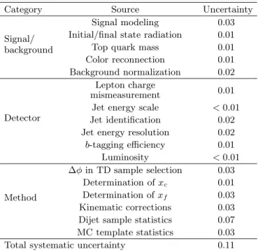
The systematic uncertainties on the fraction f are listed in Table II, and are classified in three categories: uncertainties related to (i) modeling of signal and back-ground events; (ii) simulation of detector response; and (iii) analysis procedures and methods. The maximum likelihood fit is repeated for each systematic source using the templates modified by the systematic effect, and the resulting deviation from the nominal value is taken as the corresponding systematic uncertainty.

The largest uncertainty, of 0.07, is due to the limited size of the selected dijet samples used to model the charge templates for b-quark jets. Several systematic sources

TABLE II: Summary of systematic uncertainties on the frac-tion f of SM top quarks. The uncertainties are given in units of absolute value.

Category Source Uncertainty

Signal/ background

Signal modeling 0.03 Initial/final state radiation 0.01

Top quark mass 0.01

Color reconnection 0.01 Background normalization 0.02 Detector Lepton charge 0.01 mismeasurement

Jet energy scale < 0.01 Jet identification 0.02 Jet energy resolution 0.02 b-tagging efficiency 0.01 Luminosity < 0.01 Method ∆φ in TD sample selection 0.03 Determination of xc 0.01 Determination of xf 0.03 Kinematic corrections 0.03 Dijet sample statistics 0.07 MC template statistics 0.03 Total systematic uncertainty 0.11

yield uncertainties on the measurement at the ≈ 3% level, such as (i) the determination of xf, reflecting differences in the mixing parameters and decay rates of B hadrons between the simulation and their latest experimental val-ues [26], (ii) the parametrization of the corrections for kinematic differences in the distributions of jet charge for the dijet and t¯t samples, and (iii) modeling of signal, where the effects of higher-order corrections, parton evo-lution, and hadronization are estimated using t¯t events simulated with mc@nlo [27] interfaced with herwig [28] for parton evolution.

The maximum likelihood fit to the top quark charge distribution in data yields the fraction f = 0.88 ± 0.13 (stat)±0.11 (syst). We employ the ordering-principle suggested by Feldman and Cousins [29] to set limits on f . The total uncertainty, i.e., the quadratic sum of the statistical and systematic uncertainties in Table II, is as-sumed to be a Gaussian distribution in f . For the ob-served value, we find that the hypothesis that all top quarks in the data are BSM quarks is excluded at greater than 5 SD, as shown in Fig. 4, which is consistent with

the results obtained from the likelihood ratio. We also find a lower limit of f = 0.54 at a 95% CL, which cor-responds to an equivalent upper limit on the fraction of BSM quarks of f ≤ 0.46 at the same level of significance. In summary, using b-tagged jets in lepton+jets t¯t events in 5.3 fb−1 of p¯p data, we test the hypothesis that the particle assumed to be the SM top quark has an elec-tric charge of −4/3 e. We exclude the possibility that all observed top quarks are BSM quarks at the level of more than 5 SD. We also consider a possible admixture of such

meas

f

f

FIG. 4: (color online) Confidence belts from the Feldman-Cousins approach for 1 SD (dark green), 3 SD (light green), and 5 SD (yellow). The red solid line shows the average of the measured values fmeas for each input fraction ftrue and

the vertical dashed line represents the fraction (f = 0.88) observed in the data.

quarks with the SM top quarks and place an upper limit of 0.46 on the fraction of BSM quarks at a 95% CL. The observed charge of the top quarks is in good agreement with the standard model.

We thank the staffs at Fermilab and collaborating in-stitutions, and acknowledge support from the DOE and NSF (USA); CEA and CNRS/IN2P3 (France); MON, NRC KI and RFBR (Russia); CNPq, FAPERJ, FAPESP and FUNDUNESP (Brazil); DAE and DST (India); Col-ciencias (Colombia); CONACyT (Mexico); NRF (Ko-rea); FOM (The Netherlands); STFC and the Royal So-ciety (United Kingdom); MSMT and GACR (Czech Re-public); BMBF and DFG (Germany); SFI (Ireland); The Swedish Research Council (Sweden); and CAS and CNSF (China).

[1] F. Abe et al. (CDF Collaboration), Phys. Rev. Lett. 74, 2626 (1995); S. Abachi et al. (D0 Collaboration), Phys. Rev. Lett. 74, 2632 (1995).

[2] D. Chang, W. Chang and E. Ma, Phys. Rev. D 59, 091503 (1999);

[3] D. Chang, W. Chang and E. Ma, Phys. Rev. D 61, 037301 (2000); D. Choudhury, T.M.P. Tait, and C.E.M.

Wagner, Phys. Rev. D 65, 053002 (2002).

[4] G. Aad et al. (ATLAS Collaboration), Eur. Phys. J. C 73_{, 2261 (2013); S. Chatrchyan et al. (CMS} Collabo-ration), Eur. Phys. J. C 73, 2339 (2013); V. Abazov et al. (D0 Collaboration), submitted to Phys. Rev. D (arXiv:1401.5785 [hep-ex]); T. Aaltonen et al. (CDF Col-laboration), Phys. Rev. Lett. 110, 121802 (2013).

[5] V. Abazov et al. (D0 Collaboration), Phys. Rev. Lett. 98_{, 041801 (2007).}

[6] T. Aaltonen et al. (CDF Collaboration), Phys. Rev. D 88_{, 032003 (2013).}

[7] G. Aad et al. (ATLAS Collaboration), J. High Energy Phys. 11 (2013) 031.

[8] S. Snyder, “Measurement of the Top Quark mass at D0”, Doctoral Thesis, State University of New York at Stony Brook (1995). FERMILAB-THESIS-1995-27.

[9] R. Field and R. Feynman, Nucl. Phys., B 136, 1 (1978). [10] V. Abazov et al. (D0 Collaboration), Nucl. Instrum.

Meth. A 565, 463 (2006).

[11] The pseudorapidity is defined as η = − ln[tan(θ/2)], where θ is the polar angle with respect to the beam axis measured at the center of the detector.

[12] S. Abachi et al. (D0 Collaboration), Nucl. Instrum. Meth. A 338, 185 (1994).

[13] V. Abazov et al. (D0 Collaboration), Nucl. Instrum. Meth. A 552, 372 (2005).

[14] V. Abazov et al. (D0 Collaboration), Phys. Rev. D 84, 012008 (2011).

[15] G. Blazey et al., in Proceedings of the Workshop: “QCD and Weak Boson Physics in Run II”,edited by U. Baur, R.K. Ellis, and D. Zeppenfeld, Fermilab-Pub-00/297 (2000).

[16] V. Abazov et al. (D0 Collaboration), Nucl. Instrum. Meth. A 620, 490 (2010). In this paper, jets with NN > 0.65 are tagged.

[17] M. L. Mangano et al., J. High Energy Phys. 07 (2003) 001. We use version v2.11.

[18] T. Sj¨ostrand, S. Mrenna and P. Skands, J. High Energy Phys. 05 (2006) 26. We use version v6.409.

[19] R. Brun and F. Carminati, CERN Program Library Long Writeup W5013, 1993 (unpublished).

[20] E. Boos et al. (CompHEP Collaboration), Nucl. Instrum. Meth. A 534, 250 (2004).

[21] V. Abazov et al. (D0 Collaboration), Phys. Rev. D 76, 092007 (2007).

[22] M. Czakon et al., Phys. Rev. Lett. 110, 252004 (2013). [23] The dijet sample is a subset of the data sample collected

with an additional layer of the D0 silicon system (R. Angstadt et al., Nucl. Instrum. Meth. A 622, 298 (2010)) corresponding to 4.3 fb−1 _{of integrated luminosity. The}

effect of this additional layer is estimated from the sim-ulation and taken into account in obtaining the charge templates for the first 1.0 fb−1 _{of events collected}

with-out this layer.

[24] Using such simulations, we find that the charge-flipping fraction has contributions of 0.23 from cascade decays, 0.11 from neutral B meson mixings, and 0.01 from misidentified electric charge.

[25] The two observables are expected to have the same dis-tributions. However, two tagged jets are statistically in-dependent and thus no strong correlation is expected. [26] J. Beringer et al. (Particle Data Group), Phys. Rev. D

86_{, 010001 (2012).}

[27] S. Frixione and B.R. Webber, J. High Energy Phys. 06 (2002) 029. We use version v3.4.

[28] G. Corcella et al., J. High Energy Phys. 01 (2001) 010. We use version v6.510.

[29] G. Feldman and R. Cousins, Phys. Rev. D 57, 3873 (1998).