HAL Id: hal-01886882
https://hal.archives-ouvertes.fr/hal-01886882
Submitted on 26 Oct 2018
HAL is a multi-disciplinary open access
archive for the deposit and dissemination of
sci-entific research documents, whether they are
pub-lished or not. The documents may come from
teaching and research institutions in France or
abroad, or from public or private research centers.
L’archive ouverte pluridisciplinaire HAL, est
destinée au dépôt et à la diffusion de documents
scientifiques de niveau recherche, publiés ou non,
émanant des établissements d’enseignement et de
recherche français ou étrangers, des laboratoires
publics ou privés.
morphology-based identification of benthic communities
across different regional seas
Abigail Cahill, John Pearman, Angel Borja, Laura Carugati, Susana Carvalho,
Roberto Danovaro, Sarah Dashfield, Romain David, Jean-Pierre Feral, Sergej
Olenin, et al.
To cite this version:
Abigail Cahill, John Pearman, Angel Borja, Laura Carugati, Susana Carvalho, et al.. A
compara-tive analysis of metabarcoding and morphology-based identification of benthic communities across
different regional seas. Ecology and Evolution, Wiley Open Access, 2018, 8 (17), pp.8908-8920.
�10.1002/ece3.4283�. �hal-01886882�
8908
|
www.ecolevol.org Ecology and Evolution. 2018;8:8908–8920. Received: 30 June 2017|
Revised: 17 April 2018|
Accepted: 20 May 2018DOI: 10.1002/ece3.4283
O R I G I N A L R E S E A R C H
A comparative analysis of metabarcoding and morphology-
based identification of benthic communities across different
regional seas
Abigail E. Cahill
1,2| John K. Pearman
3| Angel Borja
4| Laura Carugati
5|
Susana Carvalho
3| Roberto Danovaro
5,6| Sarah Dashfield
7| Romain David
1|
Jean-Pierre Féral
1| Sergej Olenin
8| Andrius Šiaulys
8| Paul J. Somerfield
7|
Antoaneta Trayanova
9,10| Maria C. Uyarra
4| Anne Chenuil
11Institut Méditerranéen de Biodiversité et d’Ecologie marine et continentale (IMBE), Aix Marseille Univ, Avignon Université, CNRS, IRD, IMBE, Marseille,
France
2Biology Department, Albion College, Albion, Michigan, USA
3King Abdullah University of Science and Technology (KAUST), Red Sea Research Center, Thuwal, Saudi Arabia 4AZTI, Marine Research Division, Herrera Kaia, Pasaia, Spain
5Dipartimento di Scienze della Vita e dell’Ambiente, Università Politecnica delle Marche, Ancona, Italy 6Stazione Zoologica “A. Dohrn”, Villa Comunale, Napoli, Italy
7Plymouth Marine Laboratory, Plymouth, UK
8Marine Research Institute, Klaipėda University, Klaipėda, Lithuania 9Nikola Vaptsarov Naval Academy, Varna, Bulgaria
10Institute of Oceanology (IO-BAS), Bulgarian Academy of Sciences, Varna, Bulgaria
This is an open access article under the terms of the Creative Commons Attribution License, which permits use, distribution and reproduction in any medium, provided the original work is properly cited.
© 2018 The Authors. Ecology and Evolution published by John Wiley & Sons Ltd.
Correspondence
Abigail E. Cahill, Biology Department, Albion College, Albion MI 49224.
Email: [email protected]
Funding information
Seventh Framework Programme, Grant/ Award Number: 308392; Saudi Aramco— KAUST Center for Marine Environmental Observations (SAKMEO); Spanish programme for Talent and Employability; Albion College
Abstract
In a world of declining biodiversity, monitoring is becoming crucial. Molecular meth-ods, such as metabarcoding, have the potential to rapidly expand our knowledge of biodiversity, supporting assessment, management, and conservation. In the marine environment, where hard substrata are more difficult to access than soft bottoms for quantitative ecological studies, Artificial Substrate Units (ASUs) allow for standard-ized sampling. We deployed ASUs within five regional seas (Baltic Sea, Northeast Atlantic Ocean, Mediterranean Sea, Black Sea, and Red Sea) for 12–26 months to measure the diversity and community composition of macroinvertebrates. We iden-tified invertebrates using a traditional approach based on morphological characters, and by metabarcoding of the mitochondrial cytochrome oxidase I (COI) gene. We compared community composition and diversity metrics obtained using the two methods. Diversity was significantly correlated between data types. Metabarcoding of ASUs allowed for robust comparisons of community composition and diversity, but not all groups were successfully sequenced. All locations were significantly dif-ferent in taxonomic composition as measured with both kinds of data. We recovered
1 | INTRODUCTION
To effectively conserve biodiversity at all levels of biological organi-zation, the first crucial step is monitoring and assessment (Patrício et al., 2016). However, monitoring in some habitats remains difficult (Carugati, Corinaldesi, Dell’Anno, & Danovaro, 2015). The hard- bottom subtidal zone of the marine environment can be monitored using technologically advanced, often costly, methods (e.g., in situ chambers and equipment) or time- consuming scientific diving. Thus, our knowledge about the effects of human pressures on these com-munities is still limited. Increasing this understanding is a priority, and requires both implementing innovative measures to monitor ma-rine biodiversity and developing standardized protocols (Danovaro et al., 2016).
In addition, identifying the species present in subtidal habitats is not always easy. Monitoring hard- bottom organisms typically quires the morphological identification of species. This method re-quires specialized expertise and is too time- consuming and costly for routine monitoring, especially at large scales (Carugati et al., 2015; Ferraro, Cole, DeBen, & Swartz, 1989; McManus & Katz, 2009). The use of traditional taxonomy is also complicated by the presence of cryptic species, which are genetically distinct but morphologically indistinguishable (Knowlton, 1993, 2000), or by cryptic develop-mental stages (Pfenninger & Schwenk, 2007).
Alternatively, molecular metabarcoding has been proposed as a promising method to rapidly measure the community composition based on the genetic identification of species in an area (Bourlat et al., 2013; Cristecu, 2014; Taberlet, Coissac, Pompanon, Brochmann, & Willerslev, 2012). Recent studies have quantified biodiversity using metabarcoding techniques in many habitats (e.g., Andersen et al., 2012; Yu et al., 2012). Molecular data may also be able to identify members of the community that are present in the guts of larger organisms, which otherwise would be impossible to identify based on morphology. In recent years, molecular metabarcoding has been increasingly recognized for its potential contribution to the study of marine biodiversity (e.g., Brannock, Ortmann, Moss, & Halanych, 2016; Bucklin, Lindeque, Rodriguez- Ezpeleta, Albaina, & Lehtiniemi, 2016; Kelly et al., 2017; Lejzerowicz et al., 2015; Leray & Knowlton,
2015; Pearman, Anlauf, Irigoien, & Carvahlo, 2016; de Vargas et al., 2015). Molecular techniques and the use of a single barcoding gene allow for rapid identification of specimens in marine communities (Danovaro et al., 2016). Although metabarcoding is a highly prom-ising technique, it has its drawbacks as well, including sensitivity of the results to marker choice and the fact that reference databases are incomplete (Carugati et al., 2015; Danovaro et al., 2016; Deagle, Jarman, Coissac, Pompanon, & Taberlet, 2014; Deiner et al., 2017).
Standardized sampling methods and analytical protocols and techniques for marine habitats are highly desirable for reliable de-scriptions of biodiversity and community composition (Hering et al., 2018). Hard- bottom marine substrata cannot be sampled using the same methods that have been developed in other habitats (e.g., grabs, Danovaro et al., 2016). To standardize sampling in these areas, Artificial Substrate Units (ASUs) such as nylon pan scourers can pro-vide a standardized volume and have been used to quantitatively sample early life stages of target taxa, or to experimentally ma-nipulate and sample whole communities (Gobin & Warwick, 2006; Hale, Calosi, McNeill, Mieszkowska, & Widdicombe, 2011; Kendall et al., 1996; Menge, Berlow, Blanchette, Navarrete, & Yamada, 1994; Menge, Chan, Nielsen, Di Lorenzo, & Lubchenco, 2009; Menge et al., 2002; Underwood & Chapman, 2006). These ASUs mimic algal hold-fasts or seagrasses (Kendall et al., 1996; Menge et al., 1994; Paine, 1974) and the small mesh size allows for the sampling of small- bodied taxa. ASUs may therefore target a different set of taxa than would be sampled when using hard settlement plates or Autonomous Reef Monitoring Structures (ARMS) (e.g., Leray & Knowlton, 2015; Pearman et al., 2016; Pearman et al., 2018). Other studies, including some conducted in the marine environment, have used morphology and metabarcoding to analyze communities (e.g., Cowart et al., 2015; Kelly et al., 2017; Lejzerowicz et al., 2015), but few studies exist that compare these methods in hard- bottom environments.
In this study, we use ASUs and both metabarcoding and tradi-tional morphological analysis to explore benthic communities. Our goals were both to compare metabarcoding and morphological analysis in assessing benthic diversity patterns and to evaluate the suitability of using our sampling and analysis protocols in several regional seas. Sampling was undertaken in seven geographically previously known regional biogeographical patterns in both datasets (e.g., low spe-cies diversity in the Black and Baltic Seas, affinity between the Bay of Biscay and the Mediterranean). We conclude that the two approaches provide complementary infor-mation and that metabarcoding shows great promise for marine monitoring. However, until its pitfalls are addressed, the use of metabarcoding in monitoring of rocky ben-thic assemblages should be used in addition to classical approaches rather than in-stead of them.
K E Y W O R D S
Artificial Substrate Unit (ASU), COI, innovative monitoring, marine invertebrates, metabarcoding
widespread locations (Table 1, Figure 1), and we used both morpho-logical and molecular methods to identify the macroinvertebrates found in these locations. We chose the mitochondrial gene COI as our barcoding gene, as it is one of the preferred loci for “universal”
barcoding (Lorenz, Jackson, Beck, & Hanner, 2005), has a large ref-erence database, is highly variable between species, and has been already used in previous studies to assess benthic metazoan biodi-versity (e.g., Leray & Knowlton, 2015). Both methods (morpholog-ical and molecular) were used to measure taxonomic richness and diversity and community composition with the hope of making recommendations for future monitoring programs. In addition, our sampling design allowed us to evaluate the effectiveness of the two methods in distinguishing biogeographic patterns among regions and whether or not these methods are viable in a wide range of seas.
2 | METHODS
2.1 | Artificial substrate units: deployment and
recovery
ASUs were composed of four nylon pan scourers fastened together, attached to a stainless- steel rod using a cable tie, and affixed to the substratum. We selected six sampling locations in five regional seas (Table 1, Figure 1). Within each of the six sampling locations, we chose three sites, with three ASUs deployed per site, for a total of nine per location. Samples were also available from a single site in the English Channel, our seventh location. Sites ranged from 7 to 19 m depth; most sites were between 7 and 12 m. ASUs were deployed between May 2013 and June 2014, and nearly all stayed in the field 12–14 months. Differences in deployment dates and lengths of deployment time are explained by weather and resource limitations that hindered boat and diving activity. Most notably,
TA B L E 1 Sampling sites. Details of sampling sites, including the location, site name, depth of deployment, dates of deployment and
recovery, and the number of Artificial Substrate Units (ASUs) recovered. All sites started with 3 ASUs
Location Site Latitude Longitude Depth (m) Date deployed Date recovered N recovered
Baltic Sea Karkle 55°47.352 N 21°2.518 E 8 June 2013 August 2015 1
Baltic Sea Palanga 55°55.57 N 21°1.598 E 8 June 2013 August 2015 2
English Channel Gugh Reef 49°53.180 N 06°19.345 W 19 May 2013 April 2014 2
Bay of Biscay Lekeitio 43°22.311 N 2°30.258 W 12 June 2013 July 2014 1
Bay of Biscay Pasaia 43°20.231 N 1°55.638 W 11 May 2013 May 2014 2
Bay of Biscay Zumaia 43°18.748 N 2°13.641 W 11 May 2013 June 2014 3
Gulf of Lions Cassidaigne 43°8.740 N 5°32.740 E 17 July 2013 December 2014 3
Gulf of Lions Elvine 43°19.780 N 5°14.210 E 17 June 2013 December 2014 3
Gulf of Lions Rioux Sud 43°10.370 N 5°23.420 E 17 June 2013 December 2014 3
Adriatic Sea Due Sorelle 43°32.953 N 13°37.699 E 9 June 2014 July 2015 3
Adriatic Sea Grotta
Azzurra
43°37.313 N 13°31.691 E 7 June 2014 July 2015 2
Adriatic Sea La Scalaccia 43°36.291 N 13°33.102 E 9 June 2014 July 2015 2
Black Sea Aladja Bank 43°16.800 N 28°03.396 E 7 August 2013 September 2014 1
Black Sea Cherni Nos 42°55.650 N 27°54.637 E 7 August 2013 September 2014 2
Black Sea Kamchia 43°01.114 N 27°54.129 E 8 August 2013 September 2014 1
Red Sea Janib Sa’ara
Reef
21°27.253 N 39°06.661 E 10 April 2013 June 2014 1
Red Sea Qaham Reef 21°04.921 N 39°12.063 E 10 April 2013 June 2014 3
F I G U R E 1 Map of sampling locations. The seven locations
within five regional seas sampled in this study. Locations were sampled at multiple sites, with multiple artificial sampling units per site. Complete sampling information is listed in Table 1
due to exceptional bad weather in the Baltic Sea, recovery of the samples in this location was not possible until after 26 months. The ASUs needed to be reinstalled in the Adriatic Sea following loss due to rough sea conditions. All ASUs were collected between May 2014 and August 2015. Divers recovered the ASUs, placing them in containers at the collection site underwater to prevent loss of material and returned immediately to the laboratory, where the samples were stored in ethanol (except for those from the English Channel, which were stored in formalin). Not all replicates were recovered at all sites. Table 1 contains the complete sampling and location information.
2.2 | Morphological data collection
In the laboratory, we separated the four pan scourers that made up each ASU and removed the mobile animals. We shook each scourer vigorously in deionized water to remove loose material, and then cut it open to pick out material that remained stuck in the mesh. We sieved the material from each scrubber on a 40 μm mesh and visually sorted it to collect animals larger than approximately 1 mm, which were then
preserved in ethanol. Following the sorting procedure, specimens were identified to a standard taxonomic level (usually class) based on morphological characters and we counted the number of individuals belonging to each taxonomic group. The full list of groups identified with morphological sorting is available in Supporting Information Appendix S1. A single person did the sorting to minimize observer bias, but this limited our ability to identify taxa more precisely over the large geographic scale of the study. Within each taxonomic group, we focused on the lowest level of classification that could easily and rapidly be identified. Limiting the taxonomic resolution at this step limits the precision of biological conclusions that we can draw from our data, but allowed us to compare data collected with morphological and molecular methods given a roughly equal time investment. After identification, specimens were pooled into phylum- level groups, and the biomass for each group was measured. Five groups were used for each sample: annelids, arthropods, echinoderms, molluscs, and “other” (animals that did not fit into one of the four preceeding groups).
2.3 | Metabarcoding protocol
All samples were then analyzed using a metabarcoding approach (excepting those from the English Channel, which had been stored in formalin). After calculating biomass, the phylum- level groups were ground using a mortar and pestle. Phylum- specific extractions were used to reduce overrepresentation of large- bodied (Elbrecht, Peinert, & Leese, 2017) or extremely common organisms in the se-quencing (e.g., amphipods in the Bay of Biscay). We extracted DNA from up to 0.4 g of mixed tissue using Machery- Nagel NucleoSpin®
96 Tissue Kits. Separate extractions were performed for each phy-lum of each sample, for a total of 151 individual extractions. The amount of DNA in each extraction was quantified with fluorometry using a Qubit 2.0 (Invitrogen).
We pooled the DNA from all phyla for a single sample in equi-molar concentrations (i.e., most samples contained DNA from five different extractions) and quantified the DNA in the pools using a Qubit 2.0. We chose to use the mitochondrial gene COI as our barcoding gene, due to its large reference database and other rea-sons described above. We used PCR to amplify the mitochondrial (mt) COI barcodes from the pools, using approximately 5 ng DNA, 10 μl Phusion® High- Fidelity master mix (New England BioLabs),
and 0.4 μl each of the forward and reverse primers for each 20 μl reaction. We used primers from Leray et al. (2013), which were de-veloped for metabarcoding of metazoans (Leray & Knowlton, 2015; Leray et al., 2013). We conducted three replicate PCRs on each sam-ple pool using the following PCR program: 3 min at 98°C, 27 cycles (10 s 98°C, 30 s 46°C, 45 s 72°C), 5 min at 72°C. We verified ampli-fication for each replicate visually on a 1.5% agarose gel, pooled the replicates together, and then sent the pooled PCR product to the ICM- Brain and Spine Institute (Paris, France) for final library prepa-ration prior to sequencing. This prepaprepa-ration included a second PCR for the addition of adapters used in Illumina sequencing; libraries were prepared using a TruSeq HT kit. Negative controls were run during the PCR, but due to the lack of DNA in these samples, they
F I G U R E 2 Total individuals and biomass removed from Artificial
Substrate Units (ASUs). The total number of individuals (a) and biomass (b, in grams) removed from the ASUs in each of seven locations. Letters indicate significant differences among locations at the p < 0.05 level following Tukey’s HSD tests and each point represents one ASU
were not added to the sequencing run according to sequencing cen-ter protocols. Samples were sequenced using 250 bp paired- end se-quencing on an Illumina MiSeq. The raw sequences were deposited in the NCBI Short Read Archive (SRA) under the accession number SRP093498.
2.4 | Bioinformatic analysis
Raw reads from the sequencing run were automatically demulti-plexed. The paired ends were joined with a minimum of 50 bp and a maximum difference of 10% in QIIME (Caporaso et al., 2010) and quality- checked with split libraries using a Phred score of 24. Further quality filtering and the removal of primers from the reads was undertaken in mothur (Schloss et al., 2009) using trim.seqs (pdiffs = 0, maxhomop = 8, maxambig = 0). Using the trie function in pick_otus.py (QIIME), unique sequences were produced. The refer-ence sequrefer-ences produced in this step were aligned and preclustering was undertaken in mothur (diffs = 3). Singletons were removed (split. abund with a cutoff of 1 in mothur) and chimeras removed using u-search (Edgar, 2010). Lastly, molecular operational taxonomic units (mOTUs) based on similarity (97%) were produced using usearch (in QIIME’s pick_otus.py). Reference sequences for the mOTUs were assigned a taxonomy against the BOLD database (Ratnasingham & Hebert, 2007) using the Ribosomal Database Project method (rdp; Wang, Garrity, Tiedje, & Cole, 2007; confidence 0.5) within the as-sign_taxonomy script in QIIME. The assigned mOTUs were checked by eye for obvious contamination. Two mOTUs belonging to the Antarctic urchin genus Abatus were identified. DNA from this genus was being handled in the laboratory at the same time as the ASUs samples, so these mOTUs were classified as contamination and removed from the dataset. The number of reads per sample was rarefied multiple times (n = 100) at a depth of 8,200 reads within the QIIME framework and an mOTU table produced for diversity analyses.
2.5 | Statistical analysis
We compared community composition based on morphological identification among the seven different locations. We conducted a permutational multivariate analysis of variance (PERMANOVA) with the data, with sites nested within locations, as well as a non- metric multidimensional scaling (NMDS) analysis based on Bray–Curtis dis-tances. Data were fourth- root transformed prior to these analyses to reduce the influence of very common taxa (as in Clarke, 1993). We compared community richness (Margalef’s Index, d’) and di-versity (Simpson’s Index, 1- lambda’) among locations using nested PERMANOVAs, again with sites nested within locations. NMDS analyses were conducted using the vegan package, version 2.4- 0 (Oksanen et al., 2016), with R version 3.3.1 (R Core Team 2016), and PERMANOVAs were conducted with the PERMANOVA+ package in PRIMER (Anderson, Gorley, & Clarke, 2008; Clarke & Gorely, 2015; Clarke, Gorely, Somerfield, & Warwick, 2014).
The same analyses were conducted on the metabarcoding data from six locations (excluding the English Channel sam-ples). First, we conducted all analyses based on the mOTU table. Second, for a more direct comparison to the results obtained from morphological identifications, we collapsed the mOTU list to match the morphological data (usually to the class level) by taking the sum of all reads in each higher taxonomic group, re-moved unclassified OTUs as they did not match any morphologi-cal identification, and conducted all analyses again. This analysis also allowed us to compare the two datasets while accepting sim-ilar amounts of error: Porter and Hajibabei (2018) found that taxa were assigned to the correct order, class, or phylum 99% of the time (i.e., 99% accuracy) when using COI barcodes of ~400 bp length. The collapsed analyses are therefore direct comparisons to the morphological dataset both in terms of the categories used in the analysis and in the amount of error in the dataset (both are highly accurate). The full mOTU table, along with the higher
TA B L E 2 Community composition. PERMANOVA comparing community composition within and among locations as measured with
morphological identifications and with molecular data, both all molecular operational taxonomic units (mOTUs) considered (below left) and with mOTUs collapsed to match the morphological data (below right). Data were fourth- root transformed prior to analysis. Significant effects at p < 0.05 are highlighted in bold
Morphological data
Source of variation df MS pseudo- F p
Location 6 3,728.10 10.833 <0.001
Sites (location) 10 311.07 1.834 0.015
Error 18 169.64
Molecular data
Source of variation
All mOTUs considered mOTUs collapsed to match morphological data
df MS pseudo- F p df MS pseudo- F p
Location 5 12,291 4.109 <0.001 5 3,404.40 6.744 <0.001
Sites (location) 10 2,714.1 1.218 0.006 10 455.46 0.980 0.530
taxonomic designations used for the collapsed analyses, is avail-able in Supporting Information Appendix S2. We correlated the diversity measures calculated with the morphological and molec-ular data (all mOTUs considered).
We also collapsed the mOTUs to the phylum level by taking the sum of all reads in each phylum and correlated the number of reads recovered with the biomass for each phylum. Lastly, we tested the dissimilarity in composition between pairs of regions by computing dissimilarity matrices using Bray–Curtis distances. We calculated the matrices from the molecular and morphological data using the Relate function (Mantel tests) in PRIMER (Clarke & Gorely, 2015; Clarke et al., 2014). Two tests were performed, one comparing the morphological data to the full set of mOTUs and one to the molecular data that had been collapsed to match the morphological data.
3 | RESULTS
3.1 | Morphological identification
The number of specimens found in a single ASU ranged from 120 in the Red Sea to 9,787 in the Black Sea. There were significant dif-ferences in the number of organisms recovered among the differ-ent locations (F6,28 = 7.281, p < 0.001; Figure 2A). Tukey’s HSD tests showed that the Black Sea ASUs contained significantly more indi-viduals than all other locations. This was largely due to the prepon-derance of bivalves in the Black Sea (Supporting Information Figure S1A). The biomass of the organisms recovered from the ASUs was also different among locations (F6,28 = 11.45, p < 0.001; Figure 2B). Again, the bivalves in the Black Sea led to a greater biomass than in all other seas, as measured with Tukey’s HSD. As biomass was measured including molluscan shells, these shells contributed to high total biomass. There was no correlation between the number of specimens found and the duration of deployment of the ASUs (r = −0.224, p = 0.2).
The community composition of the ASUs was significantly dif-ferent both among locations (PERMANOVA, Table 2) and among sites nested within locations (PERMANOVA, Table 2). The NMDS analysis showed that locations with salinity >30 tended to cluster together, whereas the Black and Baltic Seas were separated on the plot (Figure 3A; stress = 0.143).
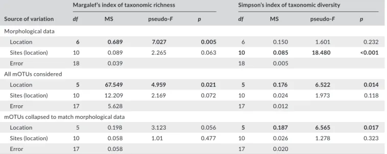
The PERMANOVA performed on Margalef’s Index of taxonomic richness showed that richness varied significantly among locations, but did not vary among sites within locations (Table 3; Figure 4A). The Black and Baltic Seas showed lower levels of richness than other locations. Taxonomic diversity, based on Simpson’s Index, showed the opposite pattern: locations were not different, but sites were different within locations (Table 3; Figure 4B). The Baltic and Red Seas, and especially the Bay of Biscay, showed a large variation in diversity among sites. Pasaia, a site found near a port in the Bay of Biscay, showed the lowest overall diversity due to an extreme abun-dance of amphipods at this site (Supporting Information Figure S1, Appendix S1).
3.2 | Metabarcoding: mOTU identification
After running the bioinformatics pipeline, the analysis recovered 1,606 unique mOTUs from 403,958 quality filtered sequences.
F I G U R E 3 Community composition in different locations.
Comparison of community composition among different locations using nonmetric multidimensional scaling analyses. Results are reported from (a) morphological identification, (b) molecular analyses (all molecular operational taxonomic units considered), (c) molecular analyses (data collapsed to match the morphological data)
Of these, 242 (15.1%) were unable to be classified based on the reference database (BOLD). The remaining mOTUs were hi-erarchically classified using rdp and reported at the class/order level in this study where possible. For a given ASU, the correla-tion between the number of reads in a phylum and the biomass of that phylum was weakly negative (r = −0.132) and not signifi-cant (p = 0.09; Figure 5). This is due in large part to the very poor recovery of bivalve sequences. Bivalves contributed a great deal to the mass of samples, particularly in the Adriatic, Baltic, and Black Seas, as described above, but were largely absent from the mOTU list (Supporting Information Figure S1). When correlations between biomass and read number were performed for each phy-lum separately, only the annelids showed a significant correlation (r = 0.505, p = 0.003).
3.3 | Metabarcoding: clustering and
diversity analyses
The community composition of the ASUs based on raw mOTU data was significantly different among locations as well as among sites within locations (PERMANOVA, Table 2). An NMDS dem-onstrated strong separation among all locations (stress = 0.196; Figure 3B). When the molecular data were collapsed to match analyses conducted on the morphological dataset, community composition was different among locations, but not among sites within locations (PERMANOVA, Table 2). An NMDS analy-sis showed much greater overlap among locations at this lower taxonomic precision, with the Black, Baltic, and Red Seas sepa-rated from the other three locations, which largely overlapped (stress = 0.218, Figure 3C).
When considering all mOTUs, the taxonomic richness varied significantly among locations, but not among sites within locations
(Table 3; Figure 6A). Richness was generally higher in the Bay of Biscay and the Gulf of Lions than other locations. Taxonomic diver-sity showed the same patterns (Table 3; Figure 6C). The Black Sea was noticeably less diverse than the other locations, although the site Karkle in the Baltic Sea also showed very low diversity. When mOTUs were collapsed to match morphological analyses, richness was not significantly different among locations or sites (Table 3; Figure 6B). Taxonomic diversity varied among locations, but not sites within locations (Table 3; Figure 6D). Sites in the Black Sea had lower diversity than other sites, and low diversity was again found at the site Karkle in the Baltic Sea (Figure 6D).
3.4 | Comparison of methods
The differences among sites in community composition resulting from morphological and molecular approaches (Table 4) were sig-nificantly related, based on Mantel tests comparing dissimilarity matrices using Bray–Curtis distances. This was true both when all mOTUs were considered (Mantel’s r = 0.638, p < 0.01) and when the molecular dataset was collapsed to match the morphological dataset (Mantel’s r = 0.748, p < 0.01).
Diversity found with the molecular analysis (all mOTUs consid-ered) was strongly correlated with the diversity obtained with the morphological analysis (r = 0.543, p = 0.001; Figure 7). The two rep-licates from Pasaia were outliers at the Biscay location in terms of high numbers of individuals and low diversity metrics based on mor-phological data (Figures 2,4,7). These samples were dominated by amphipods; pooling DNA in equimolar quantities removed this dom-inance and therefore diversity metrics calculated based on mOTUs at this site were similar to the rest of the Bay of Biscay (Figure 6). When these two outlying points were removed, the correlation in-creased (r = 0.783, p < 0.001). Diversity measured with mOTUs was
TA B L E 3 Richness and diversity. PERMANOVA of richness (left) and diversity (right) metrics among different locations. Top:
morphological identifications to the lowest possible taxonomic level (usually class). Middle: all molecular operational taxonomic units (mOTUs) were considered. Bottom: mOTUs were collapsed to match the morphological data. Significant effects at p < 0.05 are highlighted in bold
Source of variation
Margalef’s index of taxonomic richness Simpson’s index of taxonomic diversity
df MS pseudo- F p df MS pseudo- F p
Morphological data
Location 6 0.689 7.027 0.005 6 0.150 1.601 0.232
Sites (location) 10 0.089 2.265 0.063 10 0.085 18.480 <0.001
Error 18 0.039 18 0.005
All mOTUs considered
Location 5 67.549 4.959 0.021 5 0.176 6.522 0.014
Sites (location) 10 12.209 2.169 0.072 10 0.024 1.973 0.118
Error 17 5.628 17 0.012
mOTUs collapsed to match morphological data
Location 5 0.198 3.123 0.056 5 0.187 6.565 0.017
Sites (location) 10 0.058 1.01 0.477 10 0.026 1.278 0.323
generally higher than measured with morphological data, as indi-cated by a comparison to the 1:1 line (Figure 7).
4 | DISCUSSION
4.1 | Comparison of traditional and molecular
approaches
The use of both morphological and metabarcoding approaches on the same set of samples allowed us to directly compare the two methods. Despite the overall similarity of the results found with the two datasets, there were some key differences. For instance, the clustering of mOTUs at 97% similarity resulted in a much higher number of taxonomic units than the morphological approach. The higher diversity observed with molecular data has previously been observed (e.g., Dell’Anno, Carugati, Corinaldesi, Riccioni, &
Danovaro, 2015; Guardiola et al., 2016). While a higher diversity is observed in the molecular data, species assignments at the mOTU level are often currently unachievable. However, given the accuracy of the rdp classifier at coarse taxonomic scales, using a lower thresh-old for this parameter would allow the accurate assignment of tax-onomy at the same high levels as those which were undertaken for the morphological data (i.e., class; Porter & Hajibabei, 2018). Finer classifications of the morphological data are achievable, but it would require a variety of taxonomic specialists with studies focused on smaller scales.
Diversity indices calculated using both approaches were highly correlated, and community composition patterns were similar be-tween the morphological and molecular datasets based on Mantel tests performed on distance matrices. This correspondence in com-position was observed both with the full molecular dataset and when the molecular data were collapsed to match the morphological data, indicating that this result is robust across various taxonomic levels in the molecular dataset.
Despite a correspondence in overall patterns between data types, metabarcoding did not recover all groups equally. For example, bivalves made up a large proportion of both the individuals and the biomass on the ASUs as measured with morphological data but were nearly absent in molecular results (Supporting Information Figure S1, Appendices S1 and S2). This may be due to low amplification suc-cess of bivalves using these universal primers. For instance, Mytilus
galloprovincialis, a dominant species in the ASUs from the Adriatic
but one that was unrecovered during molecular analysis, has a poor mismatch to the forward primers based on sequences available in GenBank. Lejzerowicz et al. (2015) found a similar undersequenc-ing of molluscs relative to morphological data usundersequenc-ing metabarcodundersequenc-ing techniques, albeit with a different gene (18S rRNA) and different primers. Metabarcoding of COI by Leray and Knowlton (2015) using the same primers as this study found few molluscs relative to an-nelids and arthropods, but their molecular results were not directly
F I G U R E 4 Taxonomic richness and diversity among sites based
on morphological identifications. (a) Margalef’s index of taxonomic richness. (b) Simpson’s index of taxonomic diversity
F I G U R E 5 Correlation between the number of reads and the
biomass of each phylum in the Artificial Substrate Unit (ASU). Data for both mass and read number was collapsed to the phylum level, such that each point represents a phylum in a given ASU (N = 5 groups; see Methods) within a sample. Colors represent seas; shapes represent phyla
compared to morphological data. Kelly et al. (2017) found different groups of molluscs with morphological identification and COI me-tabarcoding based on eDNA samples and the Leray et al. (2013) primers. In contrast, Cowart et al. (2015) had a high sequencing rate of molluscs using Folmer primers and 454 sequencing. Ji et al. (2013) found that morphology and metabarcoding yielded similar conserva-tion recommendaconserva-tions in geographically widespread locaconserva-tions; their genetic dataset was comprised of only arthropods, again measured using Folmer primers and 454 sequencing, highlighting the fact that not all metabarcoding protocols are alike. In particular, these two sets of primers (Folmer and Leray) were developed for different rea-sons and sequencing platforms, and may strongly impact the taxa recovered via metabarcoding.
Molecular data may also contain DNA from species in larger an-imals’ guts that was not sampled via morphological analysis. The in-clusion of these gut contents can both allow us to sample taxa that are present in the community but not identifiable using morphology,
and to sample animals that are not truly part of the ASU community. Distinguishing between these two cases, or even identifying a par-ticular OTU as part of the gut contents of another organism, is not possible in this study.
Further anomalies were detected in the metabarcoding data. The two taxa that could clearly be identified as laboratory contamination (two species of Abatus urchins; see above) were removed prior to analyses. However, several potential anomalous taxa remained, par-ticularly in the samples from the Baltic Sea. These samples yielded generally lower quantities of DNA compared to other locations and were the most difficult to amplify. The low quantity of DNA may have made these samples more prone to both sequencing errors and amplification of contaminants (the Abatus mOTUs were found in these samples, for example, although all samples were amplified at the same time). Most anomalous species in the Baltic samples, par-ticularly those mOTUs that were identified as Mediterranean spe-cies and may represent cross- contamination during the laboratory
F I G U R E 6 Taxonomic richness and diversity among sites based on molecular identifications. Margalef’s index of taxonomic richness
using (a) all molecular operational taxonomic units (mOTUs) and (b) mOTUs collapsed to match the morphological data. Note the difference in the y- axis. Simpson’s index of taxonomic diversity using (c) all mOTUs and (d) mOTUs collapsed to match the morphological data
procedure, represented very low percentages of reads (<0.1%). It is unclear why the Baltic samples were the most difficult to amplify, as they were processed and stored in a manner identical to the other samples. It is possible that the DNA extractions in this region con-tained more PCR inhibitors. It is also likely that although the primers used were designed to amplify marine metazoans generally (Leray et al., 2013), the fauna of the Baltic may have more mismatches to the primers than fauna belonging to other seas, preventing reliable amplification.
Furthermore, the reference database used to identify mOTUs is limited: only species that have COI sequences in the database can be assigned to a taxon. As the reference databases are in-complete, sequenced mOTUs could actually be from organisms not present in the database. Many mOTUs could not be assigned beyond the phylum level, even in phyla where assignment to class level was possible for the morphological dataset. Filling the gaps in molecular databases will require collaboration between molec-ular ecologists and taxonomists (Bik, 2017). Given the difficulty of correctly diagnosing sources of error in mOTU identifications, we included all mOTUs except the two Abatus spp. in the analyses; this should not affect the overall validity of our clustering and di-versity analyses. However, the uncertainty of correctly assigning taxonomy to mOTUs leads us to recommend caution in the use of metabarcoding to generate a precise species list. In addition,
read number obtained with metabarcoding cannot be used as a substitute for measuring abundances or even biomass (Elbrecht & Leese, 2015; this study). These weaknesses are crucial to balance with the improved ability to detect species that may be difficult to identify in a morphological analysis (e.g., Pearman et al., 2016).
4.2 | Biogeographical patterns
In addition to comparing methods, our large sampling zone allowed us to recover known biogeographic patterns from the marine en-vironment. The seven locations investigated within these five re-gional seas showed different community composition (Supporting Information Figure S1, Figure 3). This was expected as the locations investigated ranged from the brackish, boreal Baltic Sea to the sub-tropical Red Sea. The seas considered vary in many factors, including geography, mean and seasonal temperatures, salinity, light availabil-ity, and nutrient levels. This separation was seen in the morphologi-cal data, although animals were only identified to the class level; it was also observed in the full metabarcoding dataset. When the molecular data were reanalyzed using the same level of taxonomic precision as the morphological data, the degree of separation among locations decreased (Figure 3C). However, at this level of taxonomic precision, there was still a clear separation between the Bay of Biscay, Adriatic Sea, and Gulf of Lions and the three peripheral loca-tions (Baltic, Black, and Red Seas).
Both methods identified regional patterns of biodiversity that have been previously described in the literature, further confirm-ing the efficacy of ASUs as a samplconfirm-ing device when combined with either morphological or molecular tools. For instance, we found a resemblance between the Basque coast (our sampling location in the Bay of Biscay) and the Mediterranean Sea. Fischer- Piette (1935) first described the resemblance between these two regions: the Basque coast is more like the Mediterranean than other zones in the Bay of Biscay due to summer sea surface temperatures and other biogeographical and oceanographic conditions (Borja et al., 2004).
A second previously- known pattern recovered in our data is the low diversity in the Baltic and Black Seas relative to other loca-tions (Golemanski, 2007; Ojaveer et al., 2010; Zaitsev & Mamaev, 1997). The Black Sea consistently showed low diversity and rich-ness, regardless of the dataset or metric considered. The Baltic Sea also showed lower taxonomic richness and diversity than other locations, but the diversity in the samples was more variable
Baltic Channel Biscay Gulf of Lions Adriatic Black Red
Baltic 0.530 0.610 0.723 0.626 0.457 0.572 Channel NA 0.468 0.593 0.545 0.537 0.426 Biscay 0.920 NA 0.358 0.303 0.467 0.487 Gulf of Lions 0.943 NA 0.852 0.244 0.504 0.636 Adriatic 0.918 NA 0.809 0.826 0.325 0.581 Black 0.882 NA 0.919 0.913 0.848 0.535 Red 0.891 NA 0.942 0.949 0.936 0.879 TA B L E 4 Community dissimilarities
among regions. Bray–Curtis measure of community dissimilarity based on morphological (above- diagonal elements, italics) and molecular (below- diagonal elements, all molecular operational taxonomic units considered) data. NA: not available. Numbers closer to 1 indicate higher dissimilarity between communities
F I G U R E 7 Correlation between morphological and molecular
diversity. The correlation between taxonomic diversity measured with morphological data (Simpson’s Index) and with molecular data (Simpson’s Index, all molecular operational taxonomic units considered). The solid line represents a 1:1 relationship
0.00 0.25 0.50 0.75 1.00 0.00 0.25 0.50 0.75 1.00 Morphological diversity Molecular div ersity Location Adriatic Baltic Biscay Black Gulf_of_Lions Red
than the Black Sea. Due to unfavorable diving conditions which impeded recovery, the ASUs in the Baltic Sea were immersed for nearly twice as long as in the other locations. However, the simi-lar patterns observed between the Baltic Sea and the Black Sea, where ASUs were recovered after 13 months, indicate that overall recruitment patterns are driven more by ecological and biogeo-graphic conditions (comparatively small size of the regional spe-cies pool due to low salinity, geologically younger seas, smaller basin size) than deployment times (Ojaveer et al., 2010; Zaitsev & Mamaev, 1997).
5 | CONCLUSION AND
RECOMMENDATIONS
Metabarcoding using the COI gene shows great promise as a way to monitor marine biodiversity in hard- substratum habitats, as diversity and composition metrics using metabarcoding and morphological data showed consistent results and patterns. However, based on the pres-ence of several limitations and inconsistencies in the data, we conclude that the metabarcoding technique is not yet able to replace morpho-logical identification as a monitoring tool in these habitats and make some future recommendations for researchers. First, we recommend the combined use of morphological and molecular approaches where possible; even our morphological analysis based at a low taxonomic resolution was able to identify limitations in our metabarcoding data. Second, we note that not all studies find the discrepancies that we have identified here, and urge researchers to collect preliminary data before implementing a metabarcoding- based monitoring and conser-vation plan. Such preliminary data should take into account a project’s overall goals: for instance, studies focusing on arthropods may have more success with the primer set used here than studies focusing on molluscs; studies in some locations may have greater overall success than in others (see our lower success in the Baltic Sea samples). Lastly, ASUs are small and inexpensive to deploy and process as compared to other monitoring techniques. Based on our success using them as sampling devices in hard- bottom habitats, we recommend them for long- term or high- frequency monitoring.
ACKNOWLEDGMENTS
This manuscript is a result of the DEVOTES (DEVelopment Of innovative Tools for understanding marine biodiversity and assessing good Environmental Status) project, funded by the European Union under the 7th Framework Programme, “The Ocean of Tomorrow” Theme (grant agreement no. 308392), www.devotes-project.eu. S Carvalho and JK Pearman were funded through the Saudi Aramco— KAUST Center for Marine Environmental Observations (SAKMEO). MC Uyarra was partially funded through the Spanish programme for Talent and Employability in R+D+I “Torres Quevedo.” Funding for publication was provided to AEC by Albion College. We thank the ICM- Brain and Spine Institute in Paris, France (especially Y Marie and D Bouteiller) for sequencing, U Langner for Figure 1,
and everyone who helped with the deployment and recovery of the ASUs and initial laboratory processing. We thank the editor and reviewers for their revisions, which improved earlier versions of the manuscript.
CONFLIC T OF INTEREST
None declared.
AUTHOR CONTRIBUTIONS
AEC conducted morphological identifications and molecular labora-tory work. JKP conducted the bioinformatic analyses. PS and AEC conducted the statistical analyses. AEC and JKP drafted the manu-script. AB conceived the sampling design. All authors planned the study and contributed to the field sampling, sample processing, writ-ing, and editing of the manuscript.
DATA ACCESSIBILIT Y
Raw sequence reads have been deposited at the NCBI Sequence Read Archive (SRP093498). The datasets of taxon identification (morphological and molecular) are available as supplementary materials.
ORCID
Abigail E. Cahill http://orcid.org/0000-0002-3984-7212 John K. Pearman http://orcid.org/0000-0002-2237-9723 Angel Borja http://orcid.org/0000-0003-1601-2025 Laura Carugati http://orcid.org/0000-0002-0921-6911 Romain David http://orcid.org/0000-0003-4073-7456 Susana Carvalho http://orcid.org/0000-0003-1300-1953 Sergej Olenin http://orcid.org/0000-0002-0773-1442 Paul J. Somerfield http://orcid.org/0000-0002-7581-5621 Jean-Pierre Féral http://orcid.org/0000-0001-7627-0160 Anne Chenuil http://orcid.org/0000-0001-8141-7147 Antoaneta Trayanova http://orcid.org/0000-0002-4158-1230 Maria C. Uyarra http://orcid.org/0000-0003-4509-3346
REFERENCES
Andersen, K., Bird, K. L., Rasmussen, M., Haile, J., Breuning-Madsen, H., Kjaer, K. H., … Willerslev, E. (2012). Meta- barcoding of ‘dirt’ DNA from soil reflects vertebrate biodiversity. Molecular Ecology, 21, 1966–1979. https://doi.org/10.1111/j.1365-294X.2011.05261.x Anderson, M. J., Gorley, R. N., & Clarke, K. R. (2008). PERMANOVA+ for
PRIMER: Guide to software and statistical methods (p. 214). Plymouth,
UK: PRIMER-E Ltd.
Bik, H. (2017). Let’s rise up to unite taxonomy and technology. PLoS Biology,
Borja, A., Aguirrezabalaga, F., Martínez, J., Sola, J. C., García-Arberas, L., & Gorostiaga, J. M. (2004). Benthic communities, biogeography and resources management. In A. Borja & M. Collins (Eds.), Oceanography
and marine environment of the Basque Country, Elsevier oceanography series (Vol. 70, pp. 455–492. Amsterdam, The Netherlands: Elsevier.
https://doi.org/10.1016/S0422-9894(04)80056-4
Bourlat, S. J., Borja, A., Gilbert, J., Taylor, M. I., Davies, N., Weisberg, S. B., … Obst, M. (2013). Genomics in marine monitoring: New oppor-tunities for assessing marine health status. Marine Pollution Bulletin,
74, 19–31. https://doi.org/10.1016/j.marpolbul.2013.05.042
Brannock, P. M., Ortmann, A. C., Moss, A. G., & Halanych, K. M. (2016). Metabarcoding reveals environmental factors influencing spatio- temporal variation in pelagic micro- eukaryotes. Molecular Ecology,
25, 3593–3604. https://doi.org/10.1111/mec.13709
Bucklin, A., Lindeque, P. K., Rodriguez-Ezpeleta, N., Albaina, A., & Lehtiniemi, M. (2016). Metabarcoding of marine zooplankton: Prospects, progress and pitfalls. Journal of Plankton Research, 38, 393–400. https://doi.org/10.1093/plankt/fbw023
Caporaso, J. G., Kuczynski, J., Stombaugh, J., Bittinger, K., Bushman, F. D., Costello, E. K., … Knight, R. (2010). QIIME allows analysis of high- throughput community sequencing data. Nature Methods, 7, 335–336. https://doi.org/10.1038/nmeth.f.303
Carugati, L., Corinaldesi, C., Dell’Anno, A., & Danovaro, R. (2015). Metagenetic tools for the census of marine meiofaunal biodiversity: An overview. Marine Genomics, 24, 11–20. https://doi.org/10.1016/j. margen.2015.04.010
Clarke, K. R. (1993). Non- parametric multivariate analyses of changes in community structure. Australian Journal of Ecology, 18, 117–143. https://doi.org/10.1111/j.1442-9993.1993.tb00438.x
Clarke, K. R., & Gorely, R. N. (2015). PRIMER v7: User manual/tutorial (p. 296). Plymouth, UK: PRIMER-E.
Clarke, K. R., Gorely, R. N., Somerfield, P. J., & Warwick, R. M. (2014).
Change in marine communities: An approach to statistical analysis and interpretation (3rd ed., p. 260). Plymouth, UK: PRIMER-E.
Cowart, D. A., Pinheiro, M., Mouchel, O., Maguer, M., Grall, J., Miné, J., & Arnaud-Haond, S. (2015). Metabarcoding is powerful yet still blind: A comparative analysis of morphological and molecular sur-veys of seagrass communities. PLoS One, 10, e0117562. https://doi. org/10.1371/journal.pone.0117562
Cristecu, M. (2014). From barcoding single individuals to metabarcod-ing biological communities: Towards an integrative approach to the study of global biodiversity. Trends in Ecology and Evolution, 29, 566– 571. https://doi.org/10.1016/j.tree.2014.08.001
Danovaro, R., Carugati, L., Berzano, M., Cahill, A. E., Carvalho, S., Chenuil, A., … Borja, A. (2016). Implementing and innovating marine monitor-ing approaches for assessmonitor-ing marine environmental status. Frontiers
in Marine Science, 3, 213.
de Vargas, C., Audic, S., Henry, N., Decelle, J., Mahé, F., Logares, R., … Karsenti, E. (2015). Eukaryotic plankton diversity in the sunlit ocean.
Science, 348, 1–12.
Deagle, B. E., Jarman, S. N., Coissac, E., Pompanon, F., & Taberlet, P. (2014). DNA metabarcoding and the cytochrome c oxidase subunit I marker: Not a perfect match. Biology Letters, 10, 20140562. https:// doi.org/10.1098/rsbl.2014.0562
Deiner, K., Bik, H. M., Mächler, E., Seymour, M., Lacoursière-Roussel, A., Altermatt, F., … Bernatchez, L. (2017). Environmental DNA metabar-coding: Transforming how we survey animal and plant communities.
Molecular Ecology, 26, 5872–5895. https://doi.org/10.1111/mec.14350
Dell’Anno, A., Carugati, L., Corinaldesi, C., Riccioni, G., & Danovaro, R. (2015). Unveiling the biodiversity of deep- sea nematodes through metabarcoding: Are we ready to bypass the classical taxonomy? PLoS
One, 10, e0144928. https://doi.org/10.1371/journal.pone.0144928
Edgar, R. C. (2010). Search and clustering orders of magnitude faster than BLAST. Bioinformatics, 26, 2460–2461. https://doi.org/10.1093/ bioinformatics/btq461
Elbrecht, V., & Leese, F. (2015). Can DNA- based ecosystem assessments quantify species abundance? Testing primer bias and biomass- sequence relationships with an innovative metabarcoding pro-tocol. PLoS One, 10, e0130324. https://doi.org/10.1371/journal. pone.0130324
Elbrecht, V., Peinert, B., & Leese, F. (2017). Sorting things out: Assessing effects of unequal specimen biomass on DNA metabarcoding. Ecology
and Evolution, 7, 6918–6926. https://doi.org/10.1002/ece3.3192
Ferraro, S. P., Cole, F. A., DeBen, W. A., & Swartz, R. C. (1989). Power- cost efficiency of eight macrobenthic sampling schemes in Puget Sound, Washington, USA. Canadian Journal of Fisheries and Aquatic Sciences,
46, 2157–2165. https://doi.org/10.1139/f89-267
Fischer-Piette, E. (1935). Quelques remarques bionomiques sur la côte basque française et espagnole. Bulletin du Laboratoire Maritime Saint
Servan, 14, 1–14.
Gobin, J. F., & Warwick, R. M. (2006). Geographical variation in spe-cies diversity: A comparison of marine polychaetes and nematodes.
Journal of Experimental Marine Biology and Ecology, 330, 234–244.
https://doi.org/10.1016/j.jembe.2005.12.030
Golemanski, V. (2007). Biodiversity and ecology of the Bulgarian Black Sea invertebrates. Biogeography and Ecology of Bulgaria, 82, 537–554. https://doi.org/10.1007/978-1-4020-5781-6
Guardiola, M., Wangensteen, O. S., Taberlet, P., Coissac, E., Uriz, M. J., & Turon, X. (2016). Spatio- temporal monitoring of deep- sea communi-ties using metabarcoding of sediment DNA and RNA. PeerJ, 4, e2807. https://doi.org/10.7717/peerj.2807
Hale, R., Calosi, P., McNeill, L., Mieszkowska, N., & Widdicombe, S. (2011). Predicted levels of future ocean acidification and tem-perature rise could alter community structure and biodiversity in marine benthic communities. Oikos, 120, 661–674. https://doi. org/10.1111/j.1600-0706.2010.19469.x
Hering, D., Borja, A., Jones, J. I., Pont, D., Boets, P., Bouchez, A., … Kelly, M. (2018). Implementation options for DNA- based identification into ecological status assessment under the European Water Framework Directive. Water Research, 138, 192–205. https://doi.org/10.1016/j. watres.2018.03.003
Ji, Y., Ashton, L., Pedley, S. M., Edwards, D. P., Tang, Y., Nakamura, A., … Yu, D. W. (2013). Reliable, verifiable and efficient monitoring of bio-diversity via metabarcoding. Ecology Letters, 16, 1245–1257. https:// doi.org/10.1111/ele.12162
Kelly, R. P., Closek, C. J., O’Donnell, J. L., Kralj, J. E., Shelton, A. O., & Samhouri, J. F. (2017). Genetic and manual survey methods yield dif-ferent and complementary views of an ecosystem. Frontiers in Marine
Science, 3, 283.
Kendall, M. A., Widdicombe, S., Davey, J. T. D., Somerfield, P. J., Austen, M. C. V., & Warwick, R. M. (1996). The biogeography of islands; preliminary results from a comparative study of the Isles of Scilly and Cornwall. Journal of the Marine Biological Association
of the United Kingdom, 76, 219–222. https://doi.org/10.1017/
S0025315400029155
Knowlton, N. (1993). Sibling species in the sea. Annual Review of Ecology
and Systematics, 24, 189–216. https://doi.org/10.1146/annurev.
es.24.110193.001201
Knowlton, N. (2000). Molecular genetic analysis of species bound-aries in the sea. Hydrobiologia, 420, 73–90. https://doi. org/10.1023/A:1003933603879
Lejzerowicz, F., Esling, P., Pillet, L., Wilding, T. A., Black, K. D., & Pawlowski, J. (2015). High- throughput sequencing and morphol-ogy perform equally well for benthic monitoring of marine systems.
Scientific Reports, 5, 13932. https://doi.org/10.1038/srep13932
Leray, M., & Knowlton, N. (2015). DNA barcoding and metabarcoding of standardized samples reveal patterns of marine benthic diver-sity. Proceedings of the National Academy of Sciences of the United
States of America, 112, 2076–2081. https://doi.org/10.1073/
Leray, M., Yang, J. Y., Meyer, C. P., Mills, S. C., Agudelo, N., Ranwez, V., … Machida, R. J. (2013). A new versatile primer set targeting a short fragment of the mitochondrial COI region for metabar-coding metazoan diversity: Application for characterizing coral reef fish gut contents. Frontiers in Zoology, 10, 34. https://doi. org/10.1186/1742-9994-10-34
Lorenz, J. G., Jackson, W. E., Beck, J. C., & Hanner, R. (2005). The prob-lems and promise of DNA barcodes for species diagnosis of primate biomaterials. Philosophical Transactions of the Royal Society B, 360, 1869–1877. https://doi.org/10.1098/rstb.2005.1718
McManus, G. B., & Katz, L. A. (2009). Molecular and morphological methods for identifying plankton: What makes a successful mar-riage? Journal of Plankton Research, 31, 1119–1129. https://doi. org/10.1093/plankt/fbp061
Menge, B. A., Berlow, E. L., Blanchette, C. A., Navarrete, S. A., & Yamada, S. B. (1994). The keystone species concept: Variation in interaction strength in a rocky intertidal habitat. Ecological Monographs, 64, 249– 286. https://doi.org/10.2307/2937163
Menge, B. A., Chan, F., Nielsen, K. J., Di Lorenzo, E., & Lubchenco, J. (2009). Climatic variation alters supply- side ecology: Impact of cli-mate patterns on phytoplankton and mussel recruitment. Ecological
Monographs, 79, 379–395. https://doi.org/10.1890/08-2086.1
Menge, B. A., Sanford, E., Daley, B. A., Freidenburg, T. L., Hudson, G., & Lubchenco, J. (2002). Inter- hemispheric comparison of bot-tom- up effects on community structure: Insights revealed using the comparative- experimental approach. Ecological Research, 17, 1–16. https://doi.org/10.1046/j.1440-1703.2002.00458.x
Ojaveer, H., Jaanus, A., MacKenzie, B. R., Martin, G., Olenin, S., Radziejewska, T., … Zaiko, A. (2010). Status of biodiversity in the Baltic Sea. PLoS One, 5, e12467. https://doi.org/10.1371/journal. pone.0012467
Oksanen, J., Blanchet, F. G., Friendly, M., Kindt, R., Legendre, P., McGlinn, D., … Wagner, H. (2016). vegan: Community Ecology Package. R pack-age version 2.4-0. Retrieved from https://CRAN.R-project.org/ package=vegan
Paine, R. T. (1974). Intertidal community structure. Experimental stud-ies on the relationship between a dominant competitor and its principal predator. Oecologia, 15, 93–120. https://doi.org/10.1007/ BF00345739
Patrício, J., Little, S., Mazik, K., Papadopoulou, K.-N., Smith, C., Teixeira, H., … Elliott, M. (2016). European Marine Biodiversity Monitoring Networks: Strengths, weaknesses, opportunities and threats.
Frontiers in Marine Science, 3, 161.
Pearman, J. K., Anlauf, H., Irigoien, X., & Carvahlo, S. (2016). Please mind the gap – visual census and cryptic biodiversity assessment at cen-tral Red Sea coral reefs. Marine Environmental Research, 118, 20–30. https://doi.org/10.1016/j.marenvres.2016.04.011
Pearman, J.K., Leray, M., Villalobos, R., Machida, R.J., Berumen, M.L., Knowlton, N., & Carvahlo, S. (2018). Cross-shelf investigation of coral reef cryptic benthic organisms reveals diversity patterns of the hidden majority. Scientific Reports, 8, 8090. https://doi.org/10.1038/ s41598-018-26332-5
Pfenninger, M., & Schwenk, K. (2007). Cryptic animal spe-cies are homogeneously distributed among taxa and
biogeographical regions. BMC Evolutionary Biology, 7, 121. https:// doi.org/10.1186/1471-2148-7-121
Porter, T. M., & Hajibabei, M. (2018). Automated high throughput animal COI metabarcode classification. Scientific Reports, 8, 4226. https:// doi.org/10.1038/s41598-018-22505-4
R Core Team (2016). R: A language and environment for statistical
com-puting. Vienna, Austria: R Foundation for Statistical Comcom-puting.
Retrieved from http://www.R-project.org/
Ratnasingham, S., & Hebert, P. D. N. (2007). BOLD: The barcode of life data system (www.barcodinglife.org). Molecular Ecology Notes, 7, 355–364.
Schloss, P. D., Westcott, S. L., Ryabin, T., Hall, J. R., Hartmann, M., Hollister, E. B., … Weber, C. F. (2009). Introducing mothur: Open- source, platform- independent, community- supported software for describing and comparing microbial communities. Applied and
Environmental Microbiology, 75, 7537–7541. https://doi.org/10.1128/
AEM.01541-09
Taberlet, P., Coissac, E., Pompanon, F., Brochmann, C., & Willerslev, E. (2012). Towards next- generation biodiversity assessment using DNA metabarcoding. Molecular Ecology, 21, 2045–2050. https://doi. org/10.1111/j.1365-294X.2012.05470.x
Underwood, A. J., & Chapman, M. G. (2006). Early development of sub-tidal macrofaunal assemblages: Relationships to period and timing of colonization. Journal of Experimental Marine Biology and Ecology, 330, 221–233. https://doi.org/10.1016/j.jembe.2005.12.029
Wang, Q., Garrity, G. M., Tiedje, J. M., & Cole, J. R. (2007). Naïve Bayesian classifier for rapid assignment of rRNA sequences into the new bac-terial taxonomy. Applied and Environmental Microbiology, 73, 5261– 5267. https://doi.org/10.1128/AEM.00062-07
Yu, D. W., Ji, Y., Emerson, B. C., Wang, X., Ye, C., Yang, C., & Ding, Z. (2012). Biodiversity soup: Metabarcoding of arthropods for rapid biodiver-sity assessment and biomonitoring. Methods in Ecology and Evolution,
3, 613–623. https://doi.org/10.1111/j.2041-210X.2012.00198.x
Zaitsev, Y., & Mamaev, V. (1997). Marine biological diversity in the Black
Sea. A study of change and decline. GEF Black Sea Environmental
Series. New York, NY: United Nations Publications.
SUPPORTING INFORMATION
Additional supporting information may be found online in the Supporting Information section at the end of the article.
How to cite this article: Cahill AE, Pearman JK, Borja A, et al. A
comparative analysis of metabarcoding and morphology- based identification of benthic communities across different regional seas. Ecol Evol. 2018;8:8908–8920. https://doi.org/10.1002/ ece3.4283