HAL Id: hal-00538330
https://hal.archives-ouvertes.fr/hal-00538330
Submitted on 22 Nov 2010
HAL is a multi-disciplinary open access
archive for the deposit and dissemination of
sci-entific research documents, whether they are
pub-lished or not. The documents may come from
teaching and research institutions in France or
abroad, or from public or private research centers.
L’archive ouverte pluridisciplinaire HAL, est
destinée au dépôt et à la diffusion de documents
scientifiques de niveau recherche, publiés ou non,
émanant des établissements d’enseignement et de
recherche français ou étrangers, des laboratoires
publics ou privés.
MINTCar : A tool for multiple source multiple
destination network tomography
Laurent Bobelin
To cite this version:
Laurent Bobelin. MINTCar : A tool for multiple source multiple destination network tomography.
2nd IEEE International Workshop on Internet and Distributed Computing Systems (IDCS’09), Dec
2009, jeju island, South Korea. �hal-00538330�
MINTCar : A tool for multiple source multiple
destination network tomography
Laurent Bobelin
LIP Laboratory (UMR CNRS, ENS Lyon, INRIA, UCBL 5668) GRAAL Project
46 All´ee dItalie, F-69364 Lyon Cedex 07 Email: [email protected]
Abstract—Identifying and inferring performances of a network topology is a well known problem. Achieving this by using only end-to-end measurements at the application level is known as network tomography. When the topology produced reflects capacities of sets of links with respect to a metric, the topology is called a Metric-Induced Network Topology (MINT). Tomography producing MINT has been widely used in order to predict performances of communications between clients and server.
Nowadays grids connect up to thousands communicating resources that may interact in a partially or totally coordinated way. Consequently, applications running upon this kind of platform often involve massively concurrent bulk data transfers. This implies that the client/server model is no longer valid. In this paper, we present MINTCar, a tool which is able to discover metric induced network topology using only end-to-end measurements for paths that do not necessarily share neither a common source nor a common destination.
I. INTRODUCTION
Nowadays grid testbeds often aim to link together up to thousands of computing and data storage resources over the world. Connectivity is ensured using either the Internet, or high
bandwidth.delay networks such as GEANT in Europe [1] or
TeraGrid [2] in US.
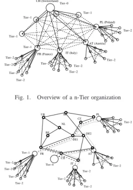
Upon such a kind of testbed, applications usually deploy software and resources dedicated to bulk data transfer. For example, EGEE project [3] uses a notion of a hierarchy of
tiers, as illustrated in figure 1. In such a hierarchy, each tier is
a data storage center physically located in one of the project partner’s lab. Level of each tier reflects the contribution of the project partner owning that resource. Tier-0 is located close to the experiment place (for EGEE, at CERN). Tier-0 communicates to tier-1, tier-1s can communicate with every tier-1s and to a subset of tier-2s and tier-2s communicate to a subset of tier-2s and a subset of tier-3s. Tier-1 are national or institutional centers, tier-2 are located close to large computing centers, tier-3 are located in labs. In such a case, the data transfer paradigm is no more a client/server one: each host is a source, a destination, or both, and each source communicates to a subset of destinations.
This logical organization is mapped into the physical ex-isting network as illustrated in figure 2. The example of the physical topology here is GEANT. As we can see, this mapping can imply that logically separated links are physically the same. For example, links between Italian and French tier-1 and between French tier-tier-1 and tier-0 are logically separated but have physically a common sub-path.
Tier−0 Tier−1 Tier−1 Tier−1 Tier−1 Tier−2 Tier−2 Tier−2 Tier−2 Tier−2 Tier−2 Tier−2 Tier−2 Tier−2 FR (France) IT (Italy) AT (Austria) PL (Poland) CH (Switzerland)
Fig. 1. Overview of a n-Tier organization
BE Tier−0 Tier−1 Tier−2 Tier−2 Tier−2 Tier−2 Tier−2 Tier−2 Tier−2 Tier−2 Tier−2 UK NL FR SE PL CZ DE1 CH DE2 IT AT
Fig. 2. Tier organization plunged into physical topology
Therefore, it is mandatory to know capacity and topology of the underlying network in order to optimize communications between tiers. If not, some logically independent transfers may compete for the same physical network resource while optimal performances would require transfers not to be scheduled simultaneously. Unfortunately, most of the time, physical topology is unknown. Moreover, existing monitoring tools like NWS [4] or WREN [5] allow to model only basic interactions between transfers. In their model, either transfers occur between hosts belonging to the same group (called
clique) and then share a common link, or not. If not, transfers
are considered as not interfering with each other.
Most of the time, the topology discovery can be done using tools like traceroute [6]. The resulting topology is unlabeled. It is formed by matching IP address of network equipments belonging to the different observed paths. However, these tools use information that can only be obtained if network administrators allow doing so. As a grid application runs on hosts owned by organizations applying different security
policies, using such tools is most of the time unrealistic. In order to infer a topology one must use only application level measurements. Such a method is known in the literature as network tomography [7].
Since a decade, network tomography has been widely studied. Different approaches have been used, depending both on the needs expressed and on targeted network (see [8] for a state of the art). Most of the time, topology is inferred using capacity of links for a given metric. This metric can be for example maximum achievable bandwidth or delay. Such a topology is an oriented graph where each edge is labeled with the capacity of the set of physical objects it represents. In client/server case, this topology is a tree. The root is the server, the leaves are clients and inner nodes are disjunction point of paths between the server and clients. Vertices are labeled with the capacity (in respect to the metric considered) of routers and wires belonging to the sub-path considered. Such inferred topologies are known as Metric Induced Network Topologies (MINT). When MINT is inferred for topologies containing paths that does not necessarily share neither the same source nor the same destination, such a topology is often name Multiple Source Multiple Destination MINT, or MSMD MINT.
This kind of topology inference is an inverse problem. Solving an inverse problem mainly consist in three steps : 1) find an accurate model for solutions, which enable to pose the problem as a well-defined one, 2) Find a way to retrieve an initial set of observed data which enables reconstruction 3) Reconstruction of the solution, given this initial set of data. For client/server case, model used is a tree, and packet train based techniques are used for the retrieval of the initial data set. Reconstruction is done most of the time using statistical techniques that aim to estimate likelihood. Roughly speaking, it consists to collapse inferred points into one when capacities of the paths leading to those inferred points are similar. These methods have drawbacks. Most of all, it relies on the assertion that the resulting topology is a tree. But as mentioned in [9], a tree cannot characterize the network when multiple sources and multiple destinations are involved.
MINTCar (Metric Induced Network Topology -
Construc-tion, Analysis and Retrieval) [10] is a new tool that performs
MSMD MINT inference using end-to-end measurements only. It is dedicated to the available bandwidth metric. It uses a network model dedicated specifically for the MSMD MINT problem, as well as dedicated algorithms and probing methods. All those models, algorithms and methods have been described in separated publications [11] [12], [13], [14]. This paper main goal is to give a general overview of this tool and by doing so give a general overview of how to deal with multiple source multiple destination tomography.
The remainder of this paper is organized as follows. First, we give an overview of existing work dealing with topology discovery in section II. We then define the terms, notations and some basic definitions of notions used in this paper in section III. We introduce the problem statement the tool solves in section IV, describe the way we probe network in section V,
and algorithms implemented for reconstruction in section VI . We finally give a general overview of MINTCar in terms of architecture and deployment in section VII, and give an overview of future work and conclude in section VIII.
II. RELATED WORK
For the classical case of a single source communicating to a set of destination, the problem has been widely studied. Different approaches have been tested. Both passive [15] and active [16] measurements have been used. It has been applied to cases such as one source communicating to many destination or many sources communicating to a single desti-nation. Reconstruction techniques are most of the time similar : they are based on statistical methods (see [8] for a state of the art). The main differences occur in the measurements procedure. Measurements are mainly realized using packet train techniques but can also be based for example on multicast trees [9].
Up to now, a few studies have focused on finding a topology for the multiple source/ multiple destination. In [17], authors use the existing MINT model to induce tree topologies. Then, they infer sub-paths common to two trees. And by this mean, they infer conjunction points between trees. The main drawback relies in the fact that ”having a common path” is not transitive. Indeed, if a path a has a common sub-path with a sub-path b, and if b has a common sub-sub-path with a path c, that does not mean that a has a common sub-path with c. Even if a has a common sub-sub-path with c, it does not mean that there is a sub-path common to all paths a,b and c. Therefore, conjunction point exists only between two trees. The method used is close to the one used in [9] where identification of common sub-path is done on edges belonging to multicast trees. More recently network coding based [18] approach have been proposed relying on the same false assumption (transitivity of ”having a common subpath” property). Other authors [19] does such a matching between trees by using harsh assumptions about the network properties, such as routing symmetry and capacity symmetry. Authors of [20] relies on routing symmetry and transitivity assumption to perform reconstruction.
In [21], authors formalize a problem close to our. The idea is to reconstruct a topology by detecting the sub-paths common to flows by using a metric related to bandwidth without labeling the edges. The notion of interference used there is close to the notion of having common detectable sub-path. Moreover, the metric used avoids any labeling.
Other authors rely on active but ”stealth” measurements (i.e. without requiring the collaboration of destinations) in order to reconstruct unlabeled topologies [22]. They use Round
Trip Time in order to infer common links between flows.
Anyhow, their method cannot infer labeled topologies, and is thus useless in our case.
III. NOTATION
A probe is the atomic action of injecting messages into the network in order to determine its properties. The complete
process of injecting probes in order to discover the entire targeted network is the measurement procedure. Hereafter in this article, we will similarly assume that routing is consistent and stable. By the former, we suppose that routing function does not allow routing paths to join, fork, and join again. By the latter, we suppose that routing paths will not change during the whole probing process. Those assumptions are most the time realistic, and so far we have not encountered problem by assuming this. This is also due because of the nature of the metric we consider, i.e. available bandwidth : most of the time, only one bottleneck is responsible for the performance of a whole path (authors of [23] proved that it should be a more or less general behavior for nowadays internet).
We consider the network as an oriented graph G = (V ∪ S∪ R, E) where vertices V are network equipments such as routers, hub, etc., S the set of hosts which will behave like senders, R the set of hosts which will behave as receivers and
E physical links between them (E ⊂ V ∪ S × V ∪ R). We
will note lij a directed edge from i to j. A host that is both
a source and a destination will be considered as two different hosts, one source and one destination.
Upon this graph, routing function defines a set of paths. If routing is consistent, there is a unique path between each source a and destination b. Indeed if two paths exists between a and b, that means that they have joined in a, then fork, and join again in b. pab is the path from a ∈ S to b ∈ R.
This path is an ordered sequence pab = {lai, lij, ljk, ..., lqb}
of directed edges lij ∈ E. We will use either link or edge in
order to name such lij. Each directed edge of any path starts
from the destination of the edge preceding it (if such an edge exists). A sub-path of pabis a sub-sequence of this sequence
that satisfies the path definition between a source a′∈ S ∪ V and a destination b′ ∈ V ∪ R. This sub-path is contained by pab. The length of a path is the number of directed edges in the
sequence. The set of all paths defined by the routing function between each source s∈ S and each destination r ∈ R will be noted Pe2e. It is the set of end-to-end paths. We will call
flow probes packets going through a path or sub-path.
A common sub-path to a set of paths Ps a sub-path
contained by each element of Ps. The common maximum
sub-path of a set of sub-paths Ps the longest common sub-path of
Ps. If consistency holds, the longest common maximum
sub-path is unique for a given Ps. This sub-path will be noted
pPs
maximum. We will say that paths contained in Ps admit a
common maximum sub-path. The set of common maximum
sub-path admitted by at least one subset of P will be noted
M axP.
A. Metric
A metric is a function whose initial domain is the set of flows and whose range is reals. As flows are defined over paths, the value obtained for a flow can label a path. We will note cp
m the capacity of a path for the metric. For example, if
the metric m is the delay, the capacity cp
m of a path will be
equal to the sum of the delay induced by each directed edge composing it.
A capacity of a path p will be detectable if there exists a set of paths containing p such that probing over those paths can exhibit capacity of p. For example, if the metric is the throughput achievable by TCP flows on steady-state, then the capacity of a sub-path can be detected only if it is feasible to saturate this path. An undetectable capacity of a path can be for example a path inducing no delay for the delay metric, or a path with infinite capacity if the metric is the bandwidth.
Hereafter in this paper, we will use the available bandwidth, noted cpbw, asMINTCaris dedicated to this metric.
B. k-detectability
Detectability as we have defined in earlier is a property of
a sub-path p. p is detectable if there is at least a subset P of Pe2e such that a probe applied to P can exhibit the capacity
of p.
Hereafter we need a more restrictive definition of
detectabil-ity in order to use it for the broader case of sub-paths shared
by a set of paths that does not necessarily share neither a common source nor a common destination. We enhance this notion by defining k-detectability. We did so because classic notion of bottleneck is defined for a single path : it is the link with the lowest capacity along the path. But for multiple paths, we needed to define exactly the sub-paths we want to consider. Roughly speaking, a k-detectable path is a path that has an influence on the path capacity when at least k flows are going through it.
k-detectability: A sub-path p is k-detectable if there is at
least one subset of P′ ⊆ P, |P′| ≤ k such that a probe applied
to P can exhibit the capacity of p.
For now, MINTCar only reconstruct 1-detectable based model of the targeted network, due to interesting properties of 1-detectability. It means that we reconstruct topology rep-resentation such that we only infer sharing of a sub-path by a set of path such that this sub-path is a bottleneck for at least one path in this set. Note that even if it is shared by other paths in P it is not necessarily a bottleneck for those paths.
IV. PROBLEM STATEMENT
(This section is devoted to the definition of the model used to describe the network and the problem statement. For further details, see [11])
A key point when trying to solve an inverse problem is the choice of the solution model. For the MSMD MINT instance of an inverse problem, this means that the model we use in order to represent the network is of crucial importance.
For former client/server work, the model is quite obvious, as under some assumptions, a tree is a more or less intuitive way to represent the network. The underlying notion that leads to the tree choice is the relation between paths. Indeed, as paths are outgoing from the same source, the relation one can quite easily probe and infer is the disjunction point between paths. Because it is possible to infer a pre-order between those disjunction points, the solution model is a pre-order, and so, a tree. But it is no longer the case when dealing with MSMD MINT : trees cannot be used in this case. Moreover,
the disjunction relation between paths does not make sense for MSMD MINT, as paths does not necessarily share neither a common source nor a destination.
Instead of using the disjunction relation, we choose to use the inclusion relation between paths and sub-paths. It means that the solution contains elements that represents paths and their sub-paths, and relations we infer between them is the inclusion of sub-paths into paths. Consider the sample network depicted figure 3. We represent here three paths all going from left to right. Inner black boxes are physical network equipments such as routers. As we are using only end-to-end measurements, most of them cannot be detected. Shaded paths are not part of the targeted platform, and so will be ignored. This lead to what is called a logical topology, depicted in figure 4. For further details concerning how to shift from real topology to the logical one, formal definition of it and formal definition of this transformation process, see [12]. For convenience, we have now named paths pa, pband pc from up
to down, and named logical links l1 to l8.
Fig. 3. Physical topology
l1 l2 l3 l4 l5 l6 l7 l8 pa pb pc
Fig. 4. logical topology
Now consider the inclusion relation between paths and sub-paths. In order to model this we will use a graph which vertices are paths and sub-paths in the logical topology, and edges are the inclusion relation. Figure 5 pictures it. Path pa, pb and pc are represented by the lower boxes with the
corresponding linestyle. pa and pb shares a common
sub-path {l4, l5}. It is depicted by the black box on the left. As
this sub-path is included in both pa and pb, there is a link
depicting this relation between this black box and each pa
and pbrepresentation. This common path contains the
sub-path common to pa, pb, pc i.e.{l5}. This common sub-path is
pc pb
pa {l4, l5}
{l5}
Fig. 5. Depicting inclusion relation
cpc bw cpb bw cpa bw c pc bw cpb bw cpa bw c pc bw cpb bw cpa bw c{l5} bw c {l5} bw c{l4,l5} bw c{l4,l5} bw
Fig. 6. Various Metric Induced Network Poset due to sub-paths capacities
depicted by the upper black box. As this sub-path is included in{l4, l5} sub-path and path pc, there is a link between each
boxes representing this path and sub-path.
For now we did not deal with any metric nor k-detectability. Now consider the available bandwidth metric. Figure 6 illus-trate different representation for the same network, that only changes due to the capacity of sub-paths and of the value of k. Left drawing corresponds to the case where both{l4, l5} and
{l5} are k-detectable. If k = 1, it means that c {l4} bw < c {l5} bw , and that c{l5} bw = c pc bw and c {l4} bw is equal to c pa bw, c pa bw or both
(i.e. because of 1-detectability definition {l4} and {l5} are
bottleneck for at least one of the paths going through it, and as l4 must be have a lower capacity than l5 in order to be
detectable).
The middle figure represents cases when l4is not detectable
anymore. This can be either the network representation of the targeted network when k= 1 and c{l4}
bw > c {l5} bw , or to k >1 and c{l4} bw greater than c pa bw and c pb
bw. Finally, the right figure
correspond to case when{l5} is not detectable, either because
k= 1 and {l5} is not a bottleneck for any path, or because it
is only detectable for k >1.
Such a representation forms a poset, so we named this model Metric Induced Network Poset, or MINP, and as its elements and labels depend on the k used for k-detectability, we named those topologies k-MINP. It can be formally defined as below.
Definition
A metric induced network poset is a poset Pm = (X, ≺) formed from M axPe2e.
• X is defined by the relation ∀i ∈ M axPe2e , i
k-detectable for the metric m ⇐⇒ i ∈ X,
• ≺ is defined by the relation ∀i, j ∈ X, i ⊂ j ⇐⇒ j ≺ i, • Every element of p∈ X is labeled by its capacity cp
This model is a key point of the whole reconstruction. In [11], we have demonstrated that the problem of reconstructing either a MINP or a k-MINP is well defined. It means that for a given network, it always exists an unique k-MINP representation for a given k. This means that if there is an algorithm able to reconstruct it from end-to-end measurements, the topology produced will be an exact representation of the network, and not an approximation of it.
V. PROBING THE NETWORK
(This section is devoted to probing methods implemented inMINTCar. For further details, see [14])
Active probing methods dealing with one source and one or many destinations widely use the well-known technique of sending back-to-back packets. Back-to-back packets are packets emitted from a source for which the last bit of a packet is followed immediately by the first bit of the next packet. Probing use either 2 (packet-pair probe) or more (packets trains) packets. The basic principle is to consider the arrival delay between successive packets. This delay is called
dispersion. We will note dispersion for a train of N packets
going through a path p ∆N p .
Our method is based on back-to-back packet trains. First aim of packet train is to measure capacity of a link. But, it has been proved by authors of [24], that if at least 80% of available bandwidth of the capacity is used by cross-traffic, then dispersion is no more reflecting capacity, but the distribution of cross-traffic through the bottleneck link.
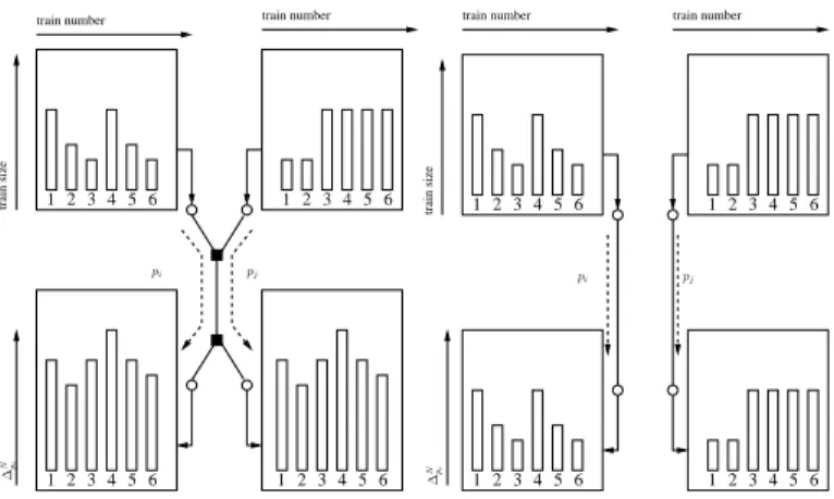
Based on this we designed a straightforward way to detect shared bottleneck as illustrated in figure 7. For each path considered, one has to estimate the available bandwidth of its bottleneck. Then, one can inject at a random time within a period T a packet train whose size varies according to a certain function which has a special distribution, different from the other path. The packets trains coming from both sources must be able, if there is a bottleneck, to use almost all its available bandwidth. Two cases are depicted : on the left, we consider the case when paths pi and pj share a bottleneck link ; on
the right, there is no such link. Packet trains (numbered 1 to 6) are injected through the paths (for the example here, we consider that they all collide, which is unlikely to happen in real life). Then we measure ∆N
pi and∆
N pj.
If there is a shared bottleneck common to the paths con-sidered, then the different trains will sometimes collide, and as a result, distribution of values for ∆N
pi and ∆
M
pj will be
dependent. The similar reasoning holds for more than two paths. Then, using accurate statistical estimator, it is possible to assess which arrival distributions depends of each other, and, by doing so, detect a shared bottleneck.
A way to determine dependency is to use information theory. Information theory and the related concepts of mutual information and independence are standard tools. We used a negentropy approximation introduced in [25] in order to determine dependency.
This gives a measurements of paths that shares a 1-detectable sub-path. In order to determine inclusion relation
2 1 3 4 5 6 2 1 3 4 5 6 2 1 3 4 5 6 2 1 3 4 5 6 train size
train number train number train number train number
2 1 3 4 5 6 2 1 3 4 5 6 2 1 3 4 5 6 2 1 3 4 5 6 train size pi pj pi pj ∆ Npi ∆ Npi
Fig. 7. Overview of the probing method
between sub-paths, we implemented the following method in
MINTCar. For a given triplet P of paths, we test if it has a1-detectable sub-paths, and determine its capacity regarding to available bandwidth. We also do that for each subset of P . It allows us to determine a1-MINP representation for this triplet, because a bottleneck of lower capacity for a set of path P′ than for a a superset of it P′′ means that P′ contains at least one more link than P′′ : the bottleneck link.
VI. RECONSTRUCTION ALGORITHM
(This section is devoted to probing methods implemented inMINTCar. For further details, see [13])
A. Useful properties
In order to reconstruct a (k-)MINP, algorithms implemented inMINTCarrely on the following properties.
Covering rule: Given a set of paths P such that|pP
max| 6=
0 no probe can exhibit two different |pP
max|. This property
trivially holds only if the metric is available bandwidth and paths are stable.
Grouping rule for bounded metrics: Let two set of paths
P = Pcore∪ {pa} ∪ Ppivot, P
′
= Pcore∪ {pb} ∪ Ppivot,
|Pcore| ≥ 0. Suppose that each elements of P all share a
common maximum sub-path, as well as elements of P′ and
Ppivot. If {pa, pb} ∪ Ppivot share a common maximum
sub-path, then P′′ = Pcore ∪ {pa} ∪ {pb} ∪ Ppivot share an
unique common maximum sub-path. Moreover if the metric is available bandwidth, then one can preorder the different common maximum sub-paths of each of those sets.
Proofs of those properties can be found in [13].
B. Algorithm overview
The overall idea is to construct a well-defined representation of a subset P of the platform, and iteratively let it grow by adding one path at a time. In order to do so, current path p relations with elements of P are tested. Because of an initial sort of paths and the fact that representation of P is well-defined, MINTCar does not have to tests relations with all elements of P , but only a few one.
• MINTCarmeasures available bandwidth for each path of the targeted platform (i.e. each path of Pe2e. This allows
to order it by increasing available bandwidth. As paths with lower capacity pass through link with lower capacity than others, it means that others cannot contain those lower capacity links. So, if there is a link common to a set of path that has a lower capacity than a path p, then p can not share it.
• MINTCariterates on the list of paths sorted by increasing capacity. It tries to measure possible relationships with existing subpaths that have already have been detected. If not, it has to measure possible interactions with all paths.
C. Performances
Complexity of this algorithm is polynomial, but this is not a key point. Unfortunately, the most expensive part of the whole MINP reconstruction is the probing of the network, which is really costly in comparison to the algorithm execution. If naive algorithms necessitate all triplets of flow to be tested, and so do 16n(n − 2)(n − 1) probes if n = |Pe2e|, we reduced it to
a best case o(n) test. We have defined in [26] ways to design algorithms using traceroute informations that have worst case scenarios costing o(n). An ongoing work is to implement them.
VII. MINTCAR:A TOOL FOR AUTOMATIC TOPOLOGY DISCOVERY
(This section is dedicated to the description of the tool, in terms of architecture, interface, and deploiement. For further information, see [10] or [26]).
A. General overview
MINTCar has been developed mainly in Java, using stan-dard Web Services as interfaces between each of its com-ponents. The core probing method is a modified version of
udpmon[27]. This tool has been extended in order to provide features such as packet train size variation using non-gaussian function, extra random time between successive sending of trains. Web services are deployed over Apache Tomcat servers [28].
An overview of the overall architecture is depicted in figure 8. Sensor User Sensor Sensor Sensor Users Storage Reconstruction Presentation Platform
Fig. 8. MINTCar : overview
Users can connect to the presentation server, that contains .jsp pages and servlets that access to the request service.
Then user can request reconstruction for a given targeted platform. Request is transmitted to the web service respon-sible for reconstruction, that schedules probes, retrieve results and actually does the reconstruction. All probing request are transmitted to a probe coordinator, that contact probing sources in order to let them do the probe.
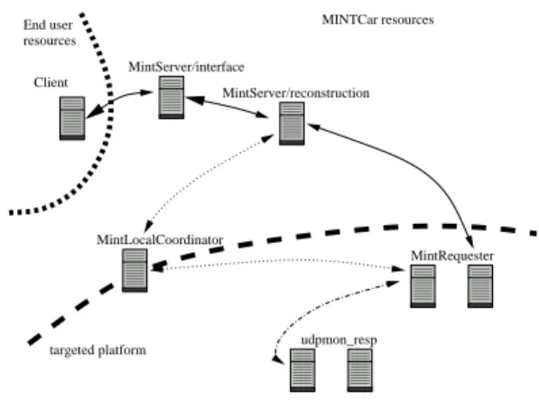
From a deployment point of view, we can separate resources necessary in 3 major groups, as depicted in figure 9.
MintRequester udpmon_resp Client MintLocalCoordinator targeted platform MintServer/interface MintServer/reconstruction
End user MINTCar resources
resources
Fig. 9. MINTCar : deployment
End users computers do not have to any software installed, as the GUI is a classic HTML interface.MINTCarresources hosts presentation and reconstruction servers. Finally sensors hosts probe coordinators, a web service that allows to request
udpmonprobing of paths, and udpmonclients and daemon.
B. Submitting a reconstruction request
As the MINP model is path-based, reconstruction request is specified by the user in a specific XML-based format containing paths description consisting in source/destination pair. End user write a file containing all paths that are paths of the targeted platform. Ongoing work aims at producing more generic targeted platform description using regular expressions describing sources and destinations.
C. Output format
Output format is an XML-based format describing targeted platform as MINP. For each path or sub-path, the XML file contains references to contained sub-paths and to bigger paths containing them.
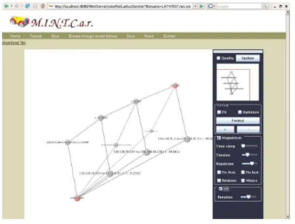
D. User interface
A screen shot of the visualization applet is given in figure 10. It allows browsing through already reconstructed MINP, submission of reconstruction requests and allows to visualize MINP in 2 or 3D.
VIII. CONCLUSION AND FUTURE WORK
In this paper we have described current version of
MINTCar, a tool for network tomography. So far, this tool propose up to our knowledge an implementation of fastest existing techniques to achieve topology reconstruction, and the
Fig. 10. A screenshot of user interface
only existing probing technique for multiple source multiple destination available bandwidth measurement.
Undergoing work has mainly three axis : enhancement of tool to support network monitoring, archiving and retrieving via a relational database, and implementation of fastest algo-rithm using multiple sources of information. The last point, indeed is a key for the success of network monitoring, as for now the tool cannot scale for large platform, due to prohibitive probing time. Using informations such as traceroute-based informations, it is possible to reduce actual probing time to less than o(n), using algorithms such as those described in [26].
ACKNOWLEDGMENT
his work has been sponsored by EGEE [3] and USS-SimGrid [29].
REFERENCES [1] “Geant website,” 2007, http://www.geant.net/. [2] “Teragrid project,” 2007, http://www.teragrid.org/. [3] “Egee project,” 2009, http://www.eu-egee.org/.
[4] R. Wolski, N. T. Spring, and J. Hayes, “The network weather service: a distributed resource performance forecasting service for metacomputing,” Future Generation Computer Systems, vol. 15, no. 5–6, pp. 757–768, 1999. [Online]. Available: citeseer.csail.mit.edu/wolski98network.html
[5] B. B. Lowekamp, N. Miller, R. Karrer, T. Gross, and P. Steenkiste, “De-sign, implementation, and evaluation of the Remos network monitoring system,” Journal of Grid Computing, vol. 1, no. 1, pp. 75–93, 2003. [6] C. Logg, L. Cottrell, and J. Navratil, “Experiences in traceroute and
available bandwidth change analysis,” presented at SIGCOMM 2004 Workshops, Portland, Oregon, 30 Aug - 3 Sep 2004.
[7] Y.Vardi, “Network tomography : estimating source-destination traffic in-tensities from link data,” Journal of the American Statistical Association, vol. 91, pp. 365–377, 1996.
[8] R. Castro, M. Coates, G. Liang, R. Nowak, and B. Yu, “Network tomography: Recent developments,” Statistical Science, 2004. [9] T. Bu, N. Duffield, F. Presti, and D. Towsley, “Network tomography on
general topologies,” uMass CMPSCI Technique Report. [10] “Mintcar project,” 2009, http://mintcar.gforge.inria.fr/.
[11] T. M. Laurent Bobelin, “Metric induced network poset (minp): a model of the network from an application point of view,” in First International
Conference on Networks for Grid Applications (GridNets), MetroGrid Workshop, October 2007.
[12] L. Bobelin and T. Muntean, “Multiple sources, multiple destinations metric induced network topology discovery: a graph theory approach,” 2006.
[13] ——, “Algorithms for network topology discovery using end-to-end measurements,” in ISPDC. IEEE Computer Society, 2008, pp. 267–274. [14] L. Bobelin, “Identifying shared bottlenecks,” in submitted to PDP, 2010. [15] V. Padmanabhan and L. Qiu, “Network tomography using passive end-to-end measurements,” dIMACS Workshop on Internet and WWW Measurement, Mapping and Modeling, Piscataway, NJ, USA, February 2002.
[16] A. Bestavros, J. Byers, and K. Harfoush, “Inference and labeling of metric-induced network topologies,” technical Report BUCS-TR-2001-010, Boston University, Computer Science Department, June 2001. [17] M. Rabbat, R. D. Nowak, and M. Coates, “Multiple source, multiple
destination network tomography.” in INFOCOM, 2004.
[18] G. Sharma, S. Jaggi, and B. Dey, “Network tomography via network coding,” in Information Theory and Applications Workshop, 2008, 27 2008-Feb. 1 2008, pp. 151–157.
[19] J. W. Byers, A. Bestavros, and K. A. Harfoush, “Inference and labeling of metric-induced network topologies,” IEEE Trans. Parallel Distrib.
Syst., vol. 16, no. 11, pp. 1053–1065, 2005.
[20] Q. Duan, W. Cai, and G. Tian, “Topology identification based on multiple source network tomography,” Intelligent Information Systems,
IASTED International Conference on, vol. 0, pp. 125–128, 2009.
[21] A. Legrand, F. Mazoit, and M. Quinson, “An application-level network mapper,” LIP, Tech. Rep. 2002-09, feb 2002.
[22] Y. Tsang, M. C. Yildiz, P. Barford, and R. D. Nowak, “Network radar: tomography from round trip time measurements.” in Internet
Measurement Conference, 2004, pp. 175–180.
[23] W. Wei, B. Wang, D. Towsley, and J. Kurose, “Model-based identifica-tion of dominant congested links,” in IMC ’03: Proceedings of the 3rd
ACM SIGCOMM conference on Internet measurement. New York, NY,
USA: ACM, 2003, pp. 115–128.
[24] C. Dovrolis, P. Ramanathan, and D. Moore, “Packet-dispersion tech-niques and a capacity-estimation methodology,” IEEE/ACM Trans.
Netw., vol. 12, no. 6, pp. 963–977, 2004.
[25] A. Hyvrinen, J. Karhunen, and E. Oja, Independent Component Analysis. John Wiley and Sons, 2001.
[26] L. Bobelin, “Tomographie depuis plusieurs sources vers de multiples destinations dans les rseaux de grilles informatiques hautes perfor-mances,” Ph.D. dissertation, Universit de la Mditerrane Aix Marseille 2, 2008.
[27] “Udpmon home page,” 2009, http://www.hep.man.ac.uk/u/rich/net/. [28] “Apache tomcat,” 2007, http://tomcat.apache.org/.