HAL Id: hal-01421417
https://hal.inria.fr/hal-01421417
Submitted on 22 Dec 2016
HAL is a multi-disciplinary open access
archive for the deposit and dissemination of sci-entific research documents, whether they are pub-lished or not. The documents may come from
L’archive ouverte pluridisciplinaire HAL, est destinée au dépôt et à la diffusion de documents scientifiques de niveau recherche, publiés ou non, émanant des établissements d’enseignement et de
Quantifying Leakage in the Presence of Unreliable
Sources of Information
Sardaouna Hamadou, Catuscia Palamidessi, Vladimiro Sassone
To cite this version:
Sardaouna Hamadou, Catuscia Palamidessi, Vladimiro Sassone. Quantifying Leakage in the Presence of Unreliable Sources of Information. Journal of Computer and System Sciences, Elsevier, 2017, 88, pp.27-52. �hal-01421417�
Quantifying Leakage in the Presence of Unreliable
Sources of Information
Sardaouna Hamadoua, Catuscia Palamidessia,1, Vladimiro Sassoneb,2
aINRIA and LIX, Ecole Polytechnique bUniversity of Southampton
Abstract
Belief and min-entropy leakage are two well-known approaches to quantify information flow in security systems. Both concepts stand as alternatives to the traditional approaches founded on Shannon entropy and mutual infor-mation, which were shown to provide inadequate security guarantees. In this paper we unify the two concepts in one model so as to cope with the frequent (potentially inaccurate, misleading or outdated) attackers’ side information about individuals on social networks, online forums, blogs and other forms of online communication and information sharing. To this end we propose a new metric based on min-entropy that takes into account the adversary’s beliefs.
Keywords: Information hiding, quantitative information flow, belief combination, probabilistic models, uncertainty, accuracy
1. Introduction
Protecting sensitive and confidential data is becoming increasingly impor-tant in many fields of human activities, such as electronic communication, auction, payment and voting. Many protocols for protecting confidential information have been proposed in the literature. In recent years the frame-works for reasoning, designing, and verifying these protocols have considered
1The work of Catuscia Palamidessi was partially supported by the INRIA Large Scale
Initiative CAPPRIS (Collaborative Action for the Protection of Privacy Rights in the Information Society).
2The work of Vladimiro Sassone was partially supported by the project Horizon 2020:
probabilistic aspects and techniques for two reasons. First, the data to be protected often range in domains naturally subject to statistical consider-ations. Second and more important, the protocols often use randomised primitives to obfuscate the link between the information to be protected and the observable outcomes. This is the case, e.g., of the DCNets [1], Crowds [2], Onion Routing [3], and Freenet [4].
From the formal point of view, the degree of protection is the converse of the leakage, i.e. the amount of information about the secrets that can be deduced from the observables. Early approaches to information hiding in literature were the so-called possibilistic approaches, in which the probabilis-tic aspects were abstracted away and replaced by non-determinism. Some examples of these approaches are those based on epistemic logic [5, 6], on function views [7], and on process calculi [8, 9]. Subsequently, however, it has been recognised that the possibilistic view is too coarse, in that it tends to consider as equivalent randomized obfuscation methods that have very di↵erent degrees of protection.
The probabilistic approaches became therefore increasingly more popu-lar. At the beginning they were investigated mainly at their strongest form of protection, namely to express the property that the observables reveal no (quantitative) information about the secrets (strong anonymity, no interfer-ence) [1, 6, 10]. Such strong property, however, is almost never achievable in practice. Hence, weaker notions of protection started to be considered. We mention in particular Rubin and Reiter’s concepts of possible innocence and of probable innocence [2] and their variants explored in [11]. These are, how-ever, still true-or-false properties. The need to express in a quantitative way the degree of protection has then lead naturally to explore suitable notions within the well-established fields of Information Theory and of Statistics.
Concepts from Information Theory [12] have proved quite useful in this domain. In particular, the notion of noisy channel has been used to model protocols for information-hiding, and the flow of information in programs. The idea is that the input s 2 S of the channel represents the information to be kept secret, and the output o 2 O represents the observable. The noise of the channel is generated by the e↵orts of the protocol to hide the link between the secrets and the observable, usually by means of randomised mechanisms. Consequently, an input s may generate several di↵erent out-puts o, according to a conditional probability distribution p(o| s). These probabilities constitute the channel matrix C. Similarly, for each output there may be several di↵erent corresponding inputs, according to the
con-verse conditional probability p(s| o) which is linked to the above by the Bayes law: p(s| o) = p(o | s) p(s)/p(o). The probability p(s) is the a priori prob-ability of s, while p(s| o) is the a posteriori probability of s, after we know that the output is o. These probability distributions determine the entropy and the conditional entropy of the input, respectively. They represent the uncertainty about the input, before and after observing the output. The di↵erence between entropy and conditional entropy is called the mutual in-formation and expresses how much inin-formation is carried by the channel, i.e. how much uncertainty about the input we lose by observing the output (i.e., equivalently, how much information about the input we gain by observing the output).
Even though several notions of entropy have been proposed in Information Theory, Shannon’s is by far the most famous of them, due to its relation with the channel’s rate, i.e., the speed by which information can be transmitted accurately on a channel. Consequently, there have been various attempts to define the degree of protection by using concepts based on Shannon entropy, notably mutual information [13, 14, 15, 16] and the related notion of capacity, which is the supremum of the mutual information over all possible input distributions, and which therefore represents the worst case from the point of view of security [17, 18, 19].
A refinement of the above approaches came from the ideas of integrating the notions of extra knowledge and belief [20, 21, 22]. The idea is that the gain obtained by looking at the output should be relative to the possible initial knowledge or belief that an attacker may have about the secret. For instance, assume that in a parliament composed by m Labourists and n Con-servatives, m members voted against a proposal to eliminate the minimum wage. Without any additional knowledge it is reasonable to believe that all Labourists voted against. If however we came to know that exactly one Con-servative voted against, then it is more reasonable to believe that the most liberally-inclined Conservative voted against, and the least liberally-inclined Labourist voted in favour. In this case, the a posteriori belief is likely to be much more accurate than the a priori one, and the gain obtained using the knowledge about MPs’ relative positioning on the left-to-right scale is much larger than the one computed as di↵erence of entropies. Consequently, [22] proposed to define the protection of a system in terms of the di↵erence (expressed in terms of Kullback-Leibler divergence) between the accuracy of the a posteriori belief and the accuracy of the a priori one.
Smith, who argued that it is not very suitable to model information leakage in the typical scenario of protocol attacks, where the adversary has only a limited number of tries to guess the value of the secret [23]. In such a sce-nario, the natural measure of the threat is the probability that the adversary guesses the right value. The case of “one-try only” was dubbed by Smith vul-nerability of the secret. Shannon entropy, on the other hand, represents the expected number of attempts that an adversary has to make to discover the secret, assuming that there is no limit to such number, and that the adver-sary can narrow down the value by probing properties of the secret. Smith gave an example of two programs whose Shannon’s mutual information is about the same, yet the probability of making the right guess after having observed the output is much higher in one program than in the other. In a subsequent paper [24], Smith proposed to define the leakage in terms of a notion of mutual information based on R´enyi min-entropy (the logarithm of the vulnerability), which captures the case of an adversary disposing of one single try. Subsequent approaches going under the name of g-leakage have extended the analysis to multiple tries, and to the case in which each guess is associated with a gain (or loss) which depends on the level of approximation [25, 26, 27]. The min-entropy approach remains however the canonical frame-work, not only for its simplicity, but also because the worst-case min-leakage (aka min-capacity) has been proved to be an upper bound to the g-leakage [25].
In [28] the authors extended the vulnerability model of [24] in the context of the Crowds protocol for anonymous message posting to encompass the frequent situation where attackers have extra knowledge. They pointed out that in Crowds the adversary indeed has extra information (viz., the target servers) and assumed that she knows the correlation between that and the secret (viz., the users’ preferences for servers). They proved that in such scenarios anonymity is more difficult to achieve.
In our opinion, a fundamental issue remains wide open: the need to mea-sure and account for the accuracy of the adversary’s extra knowledge. Indeed, [28] assumes that the adversary’s extra information is accurate, and such an assumption is generally not warranted. Inaccuracy can indeed arise, e.g. from people giving deliberately wrong information, or simply from outdated data. As already noticed in [22] there is no reason in general to assume that the probability distributions the attacker uses are correct, and therefore they must be treated as beliefs.
to cope with the presence of the attacker’s beliefs. To this end we propose a new metric based on the concept of vulnerability that takes into account the adversary’s beliefs. The idea is that the attacker does not know the actual probability distributions (i.e., the a priori distribution of the protocol’s hidden input and its correlation with the extra information), and is assuming them. The belief-vulnerability is then the expected probability of guessing the value of the hidden input in one try given the adversary’s belief. Informally, the adversary chooses the value of the secret input which has the maximum a posteriori probability according to her belief. Then the vulnerability of the secret input is expressed in terms of the actual a posteriori probabilities of the adversary’s possible choices. We show the strength of our definitions both in terms of their theoretical properties and their utility by applying them to various threat scenarios and comparing the results to the previous approaches. Among its several advantages, our model allows to identify the levels of accuracy for the adversary’s beliefs which are compatible with the security of a given program or protocol.
This paper revises and expends an earlier version [29]. First, we have sim-plified the model of the adversary’s belief. Indeed, in the previous model, an attacker’s belief consists of a pair: an assumed prior distribution over the set of secret inputs and an external channel leaking some (potentially incorrect) information about these secret inputs to the adversary. In this exposition, we simply model the belief by a subjective probability distribution, which summarises the aggregated information about the secret initially collected by the attacker from di↵erent and potentially conflicting sources of evidence. This approach is more in line with existing models of beliefs in the literature and simplifies significantly the exposition of our results and their comparison to existing work. Our approach is motivated further in §Appendix A. The flexibility of the model is illustrated in §6, where we apply our approach to di↵erent programs under various attack scenarios. We show in particular that a program which performs better than another in one threat scenario might become worse when the threat scenario evolves. Finally, exploiting notions and techniques from Dempster-Shafer Theory [30, 31], in §Appendix B we propose a new technique to estimate the reliability of an adversary’s belief. This allows us to obtain a sound method of updating an arbitrary belief applying the Bayes’ rule for updating a hypothesis.
The rest of the paper is organised as follows: in §2 we fix some basic notations and recall some fundamental notions of Information Theory; in §3 we briefly revise previous approaches to quantitative information follow;
§4 and §5 deliver our core technical contribution by extending the model on R´enyi min entropy to the case of attacker’s beliefs and investigating its theoretical properties; in§6 we apply our approach to various threat scenarios and compare it to the previous approaches; in §7 we discuss the related work whilst §8 contains our concluding remarks.
2. Preliminaries
In this section we briefly revise the elements of Information Theory which underpin the work in this paper, and illustrate our conceptual framework. 2.1. Some notions of Information Theory
Being in a purely probabilistic setting gives us the ability to use tools from information theory to reason about the uncertainty of a random vari-able and the inaccuracy of assuming a distribution for a random varivari-able. In particular we are interested in the following notions: entropy, mutual infor-mation, relative entropy and min-entropy. We refer the reader to [32, 12] for more details.
We use capital letters X, Y to denote discrete random variables and the corresponding small letters x, y and calligraphic letters X , Y for their values and set of values respectively. We denote by p(x), p(y) the probability of x and y respectively and by p(x, y) their joint probability.
Let X, Y be random variables. The (Shannon) entropy H(X) of X is defined as
H(X) = X x2X
p(x) log p(x). (1)
The entropy measures the uncertainty of a random variable. It takes its maximum value log|X | when X is uniformly distributed and its minimum value 0 when X is a constant. We take the logarithm with a base 2 and thus measure entropy in bits. The conditional entropy
H(X|Y ) = X y2Y
p(y)X x2X
p(x|y) log p(x|y) (2) measures the amount of uncertainty of X when Y is known. It can be shown that 0 H(X|Y ) H(X) with the leftmost equality holding when Y completely determines the value of X and the rightmost one when Y reveals no information about X, i.e., X and Y are independent random variables.
Comparing H(X) and H(X|Y ) give us the notion of mutual information, denoted I(X; Y ) and defined by
I(X; Y ) = H(X) H(X|Y ). (3) It is non-negative, symmetric and bounded by H(X). In other words,
0 I(X; Y ) = I(Y ; X) H(X).
The relative entropy or Kullback-Leibler distance between two probability distribution p and q on the same set X , denoted D(p k q), is defined as
D(pk q) = X x2X
p(x) logp(x)
q(x). (4)
It is non-negative (but not symmetric) and it is 0 if and only if p = q. The relative entropy measures the inaccuracy or information divergence of assuming that the distribution is q when the true distribution is p.
The guessing entropy G(X) is the expected number of tries required to guess the value of X optimally. The optimal strategy is to guess the values of X in decreasing order of probability. Thus if we assume that X = {x1, x2, . . . , xn} and xi’s are arranged in decreasing order of proba-bilities, i.e., p(x1) p(x2) · · · q(xn), then
G(X) = X 1in
ip(xi). (5)
The min-entropy H1(X) of a random variable is given by H1(X) = log max
x2X p(x) (6)
and measures the difficulty for an attacker to correctly guess the value of X in one try (obviously using the optimal strategy above). It can be shown that H1(X) H(X) with equality when X is uniformly distributed. In general, H(X) can be arbitrary higher than H1(X), since it can be arbitrary high even if X assumes a given value with probability close to 1.
2.2. Framework
In this paper we consider a framework similar to the probabilistic ap-proaches to anonymity and information flow used e.g. in [6, 33, 34], and [24]. We restrict ourselves to total protocols and programs with one high level input A, a random variable over a finite set A, and one low level output (observable) O, a random variable over a finite set O. We represent a proto-col/program by the matrix of the conditional probabilities p(oj| ai) that the low output is oj given that the high input is ai. An adversary or eavesdropper can see the output of a protocol, but not its input, and she is interested in deriving the value of the input from the observed output in one single try.
In this paper we shall assume that the high input is generated according to an a priori probabilistic distribution p(ai) unknown to the adversary, and we also denote by p (ai) the subjective probability modeling the adversary’s initial belief, as explained in the introduction3. In other words, p (ai) is her assumed a priori distribution of A.
Example 1. Let A be a random variable with an unknown (to the adver-sary) a priori distribution over A = {0, 1, 2, 3}. Suppose that A is the high input of the deterministic program C1 below, whose low output is
O = ⇢ 1 if a2 {0, 1} 2 otherwise. PROG C1: BEGIN O := b log(A + 2) c END
Now suppose that the adversary, for some reason, initially believes that A is an odd number and that 1 is more likely than 3. For example p (1) = 0.9 and p (3) = 0.1. In the case of wrong belief, i.e., when A is actually an even number, her low observation of PROG C1 does not allow her to realize that her initial belief is wrong. She will not be able to correct it and will therefore pick again the wrong value. Indeed, both observations 1 and 2 are compatible with the odd numbers. However, whereas observing O = 1
3See
§Appendix A for the rationale for representing the adversary’s belief by a subjec-tive probability distribution.
p(o | a) o0 o1 o2
a0 1 0
a1 1 0 0
a2 0 1
a3 1 0 0
Table 1: Conditional probabilistic matrix of PROG C2
would strengthen her belief that A is 1, seeing a low output of 2 might raise some doubts if the adversary does not fully trust the source of her belief, as the unlikely 3 (viz., p (3) = 0.1) has happened. In Section Appendix B we present a novel technique allowing the adversary to estimate the reliability of her initial belief and to discount it accordingly.
Now suppose that A is the high input of the probabilistic program C2 below, with low output O 2 { 1, 0, 2} and conditional probabilistic matrix as in Table 1.
PROG C2: BEGIN
R ‘sampled from {0, 2} with p(0) = and p(2) = 1 ’; If A = R
Then O := A Else O := 1 END
Contrary to the PROG C1, the low output of PROG C2 may allow the ad-versary to realize that her initial belief about the parity of A is wrong. For example if she initially believes that A is odd and then she observes that O is either 0 or 2, then she knows that her belief is wrong. But the observa-tion O = 1 does not help her to correct her inaccurate belief, as it can be induced by both even and odd numbers.
3. Uncertainty vs accuracy
This section reviews the existing definitions for quantifying information leakage. We begin by quantitative approaches to information flow based on Shannon entropy and mutual information, and recall why they fail generally to give good security guarantees. We then present alternative approaches based on the adversary’s beliefs initially proposed by Clarkson, Myers and
Schneider [22]. We conclude the section by presenting more recent alternative approaches based on the concept of vulnerability [24] and R´enyi min-entropy. 3.1. Shannon entropy approach
There seems to be a general consensus in the literature for using Shannon entropy to measure uncertainty and mutual information to quantify informa-tion leakage [35, 36, 14, 37, 33]. We remind the reader that these approaches aim at quantifying information flow as a reduction of the adversary uncer-tainty about the high input and take no account of the adversary’s initial belief. Shannon entropy H(A) as a measure of the uncertainty of A seems adequate to express the adversary’s initial uncertainty about A. Similarly, as the conditional entropy H(A| O) measures the remaining amount of uncer-tainty of A when O is known, it seems appropriate to express the adversary’s remaining uncertainty. We thus have the following definitions.
• initial uncertainty (IU): H(A)
• remaining uncertainty (RU): H(A | O)
• information leakage (IL): IU RU = H(A) H(A| O) = I(A; O) Nevertheless, recent work by Smith [24] suggests that these notions do not support security guarantees satisfactorily. In particular the remaining uncertainty is generally of little value in characterising the real threat that the adversary could guess the value of A given her low observations. Smith uses the following example to prove that.
Example 2. Consider the following programs C3 and C4, where A is a uni-formly distributed 8k-bit integer, k 2, & denotes bitwise ‘AND’, and 07k 11k+1 a binary constant. PROG C3: PROG C4: BEGIN BEGIN If A mod 8 = 0 O := A & 07k 11k+1 Then O := A END Else O := 1 END
PROG C3reveals completely the high input when A is a multiple of 8 while it reveals nothing about A otherwise (except of course the very fact that it is
not a multiple of 8). On the contrary, PROG C4 reveals always and only the last k + 1 bits of A.
According to Shannon entropy-based metrics, we have IU = 8k, RU = 7k 0.169 and IL = k + 0.169 for PROG C3, and IU = 8k, RU = 7k 1 and IL = k + 1 for PROG C4 (the reader is referred to [24] for the detailed calculations). So, under such definitions, PROG C4 appears actually worse than PROG C3, as 7k 1 < 7k 0.169, even though intuitively C3 leaves A highly vulnerable to being guessed (e.g., when it is a multiple of 8) while C4 does not, at least for large k.
3.2. Belief approach
Clarkson et al. [21, 22] showed that the Shannon entropy approach is in-adequate for measuring information flow when the adversary makes assump-tions about the high-level secret and such assumpassump-tions might be incorrect. Based on the conviction that it is unavoidable that the attacker makes such (potentially inaccurate) assumptions, they proposed a new metric. They for-malised the idea of an adversary’s belief as a distribution of A assumed by the adversary: information flow is then expressed as an improvement in the accuracy of such belief. The initial accuracy is the Kullback-Leibler distance between the adversary’s initial belief and the actual value of A; similarly the remaining accuracy is the Kullback-Leibler distance between the Bayesian-updated belief of the adversary after her low observation, and the actual value of A.
As already noticed by Smith [24], when the adversary’s belief coincides with the a priori distribution of A, then the belief approach reduces again to the inadequate standard approach illustrated above.
3.3. Vulnerability approach
Having observed that both the consensus and the belief approaches fail in general to give good security guarantees, Smith [24] proposes a new metric for quantitative information flow based on the notions of vulnerability and min-entropy. We briefly revise these concepts here.
The vulnerability of a random variable A is the worse-case probability that an adversary could guess the value of A correctly in one try. The vulnerability of A, denoted V (A), is thus formally defined as follows.
The conditional vulnerability of a A given O measures the expected prob-ability of guessing A in one try given O. It is denoted V (A| O) and defined as follows.
Definition 2. V (A| O) =Po2Op(o)V (A| o), where V (A | o) is maxa2Ap(a| o). The initial uncertainty about A is then defined as the negative logarithm of V (A), which turns out to be the min-entropy of the random variable A – cf. (6) above. The remaining uncertainty about A after observing O is defined as the min-entropy of A given O. Thus we have the following vulnerability-based definitions:
• IU : H1(A) = log V (A)
• RU : H1(A| O) = log V (A| O) • IL : IU RU = H1(A) H1(A| O)
Security guarantees of the vulnerability-based approach: by applying these definitions to the programs of Example 2, we have IU = 8k, RU = 8k 3 and IL = 3 for PROG C3, and IU = 8k, RU = 7k 1 and IL = k + 1 for PROG C4. While these quantities remain the same as in the consensus approach for PROG C4, the new metric increases the leakage ascribed to PROG C3 reflecting the fact that the low observations of PROG C3 leave the high input very vulnerable to being guessed.
4. Unifying Belief and Vulnerability
We now propose an alternative approach based on the vulnerability con-cept that takes into account the adversary’s belief.
4.1. Belief-vulnerability
Let A be a random high level variable. The belief-vulnerability of A is the expected probability of guessing A in one try given the adversary’s belief. The adversary will choose a value having the maximal probability according to her belief, that is a value a0 2 , where = argmax
a2A p (a). The vulnerability of A is then the real probability that the adversary’s choice is correct, that is the probability p(a0). As there might be many values of A in with the maximal probability, the attacker will pick uniformly at random one of them. Hence we have the following definition.
Definition 3. Let A be a random variable and = argmaxa2A p (a). The belief-vulnerability of A, denoted V (A), is defined as
V (A) = 1 | |
X a02
p(a0). (7)
The initial threat is the belief-uncertainty of A (viz. the belief min-entropy4 of A) given by the following definition.
Definition 4. Let A be a random variable. The initial threat to A, denoted H1(A), is defined as
H1(A) = log⇣ 1 V (A)
⌘
. (8)
Note that from the above definition, the initial uncertainty may be infinite when for all a in , p(a) = 0, modelling the impossibility of a correct guess in one single try when the attacker is choosing a value having zero prior probability. However it might be very difficult to quantify the decrease in uncertainty when initially it is infinite. Therefore we will assume throughout the rest of this paper that initially every value is possible, that is p(x) > 0 for all x in X .
Example 3. Suppose that A is distributed over {0, 1, 2, 3} and the adver-sary’s belief is about the parity of A.
Table 2 summarizes the initial uncertainty about A when the actual a priori distribution and the adversary’s prebelief are p1 and p2, and p 1 and p 2 respectively. The pair (p, p ) means that the actual a priori distribution of A is p while the adversary prebelief is p . Thus in (p1, p 1) the adversary believes that p1 always uniformly produces an even number while, though it usually produces e↵ectively an even number, with probability 0.02 it also produces an odd number that fools the attacker. However in a one-time guessing attack, this slightly “inaccurate” belief does not a↵ect the vulnera-bility of A as knowing p1, the actual a priori distribution, would not change the attacker choice. In (p2, p 1), on the contrary, p2 usually fools the attacker by producing an odd number while the attacker is always expecting an even
4We call it belief min-entropy since when the belief coincides with the actual a priori
(p1, p 1) (p1, p 2) (p2, p 1) (p2, p 2) V (A) 0.49 0.01 0.02 0.47 H1(A) 1.03 6.64 5.64 1.09 p⇢1 p1 p2 p 1 p 2 a0 0.49 0.03 0.5 0 a1 0.01 0.47 0 0.95 a2 0.49 0.01 0.5 0 a3 0.01 0.49 0 0.05
Table 2: Initial uncertainty in presence of belief
number. This decreases very much the vulnerability of A as it is almost im-possible for the attacker to guess the value of the secret in one try when her initial belief is so wrong. Hence, the increase in her initial uncertainty.
Next we show that the lower bound of the belief-uncertainty is obtained with a full knowledge of the actual a priori distribution (viz., a true and justifiable belief).
Theorem 1. H1(A) H1(A).
Proof. Let = argmaxa2A p (a) be the set of the adversary’s possible choices. V (A) = 1 | | X a2 p(a) 1 | | X a2 max a02Ap(a 0) ( since ✓ A) Therefore, V (A) 1 | | P
a2 V (A) = | |1 | |V (A) = V (A). Hence H1(A) H1(A).
The lower bound is reached if and only if all the adversary’s possible choices have the actual maximum a priori probability.
Proposition 1. H1(A) = H1(A) i↵ ✓ argmaxa2Ap(a).
Proof. The proof in the right direction is similar to the proof of Theorem 1 where the inequality is replaced by the equality. To see why the opposite holds, it is sufficient to observe that when there exists an element of that has not the maximum a priori probability then V (A) is less than V (A). Hence the uncertainty is greater than the lower-bound.
In particular when the prebelief coincides with the actual a priori distri-bution so are the belief min-entropy and the min-entropy.
Corollary 1. If p(a) = p (a) for all a in A, then H1(A) = H1(A).
In the vulnerability model where the adversary is supposed to know the a priori probability distribution of the high input, the minimum vulnerability, or equivalently the maximum uncertainty, is obtained using a uniform distri-bution. However in the presence of belief, the uncertainty can be arbitrary high. In fact we have the following upper-bound of the belief min-entropy. Theorem 2. H1(A) log⇣mina2Ap(a)⌘.
Proof. Similar to the proof of Theorem 1 with max replaced by min and the inequality is reversed.
In particular the belief uncertainty hits the upper-bound when all the adversary’s possible choices have the actual minimal prior probability. Proposition 2. H1(A) = log⇣mina2Ap(a)⌘ i↵ ✓ argmina2A p(a).
The proof in the right direction is again similar to the proof of Theorem 1 where the inequality is replaced by the equality and max by min. To see why the other implication holds, it is sufficient to observe that when there exists an element of that has not the minimum a priori probability then V (A) is greater than mina2Ap(a). Hence the uncertainty is less than the upper-bound.
We conclude this section by showing two interesting properties of the belief uncertainty. First, we show that beliefs have no e↵ect on the initial uncertainty of A when its actual a priori probability distribution is uniform. In that case, any choice of the attacker results in the same actual vulnerability and she has the same probability |A|1 of a correct guess.
Proposition 3. If A is uniformly distributed then for all initial belief p , we have
H1(A) = H1(A) = log⇣|A|⌘. Proof. Let = argmaxa2A p (a).
V (A) = 1 | | X a2 p(a) = 1 | | X a2 1 |A| = 1 | | X a2 V (A) = 1 | | | |V (A) = V (A). Hence H1(A) = H1(A) = log⇣|A|⌘.
Conversely, for a vacuous belief, the initial belief-uncertainty is indepen-dent of the actual a priori distribution of the high input.
Proposition 4. If the prebelief is vacuous then H1(A) = log⇣|A|⌘.
Proof. If the prebelief is vacuous then its pignistic transformation p (Lemma 4) is the uniform probability distribution. Thus = argmaxa2A p (a) =A. Therefore, V (A) = 1 | | X a2 p(a) = 1 |A| X a2A p(a) = 1 |A| X a2A 1 = 1 |A| Hence H1(A) = log⇣|A|⌘.
4.2. A posteriori belief-vulnerability
The belief-vulnerability of A given the evidence O is the expected proba-bility of guessing A in one try given the evidence. Given evidence O = o, the adversary will choose a value having the maximal conditional probability ac-cording to her belief, that is a value a0 2 o, where
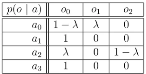
o = argmaxa2A p (a| o). But unlike the a priori belief-vulnerability, here the evidence O could contra-dict the attacker prebelief. For example assume that the adversary initially believes that the high input value is a2, that is p (a2) = 1 then she observes the output o1 of PROG C5 of which we only give the channel matrix Table 3. The evidence o1 contradict her prebelief since only a0 or a3 could produce o1. Hence her prebelief becomes vacuous and cannot be used as an a priori probability to update her belief.
p(o| a) o0 o1 o2 a0 0.99 0.01 0 a1 1 0 0 a2 0.01 0 0.99 a3 0 1 0
Table 3: Channel matrix of PROG C5
To avoid such completely wrong belief, we take the point of view that the adversary initial beliefs satisfy an admissibility restriction (see e.g. [22, 38]).
In particular, we consider an admissibility restriction we deem ✏-admissible beliefs5, where a belief never di↵ers by more that a factor of ✏ from a uniform distribution, that is, p (a) |A|✏ for all a in A. Note that the evidence o and the adversary prebelief could still be highly conflicting but never fully contradicting each other. Indeed, consider again the program PROG C5 above. If we assume that the adversary prebelief is such that p (a0) = 0.90 and p (a3) = 0.01 then her belief highly supports a0. Now observing o1 would conflict with this belief as the evidence o1 alone highly supports a3 rather than a0: a0 would more likely have produced o0. In this section, we shall assume that the adversary updates her belief using the Bayes’ rule. Thus, the a posteriori belief is
p (a| o) = p(o| a)p (a) p (o)
= P p(o| a)p (a) a02Ap(o| a0)p (a0)
which is well defined thanks to the admissibility requirement. Appendix Ap-pendix B introduces an advanced technique that takes into account the level of conflict to estimate the admissibility factor of an arbitrary belief given the evidence (i.e. the observables) induced by the channel.
The vulnerability of A given o is then the real probability that the ad-versary’s choice (viz. a value a0 2 o = argmaxa2A p (a| o) is the correct one, that is the objective conditional probability p(a0| o). Again, as there might be many values of A with the maximal conditional probability, the attacker will pick uniformly at random one element in o. Hence we have the following definition.
Definition 5. The belief-vulnerability of A given O is defined as
V (A| O) =X o2O
p(o)V (A| o), where V (A | o) = 1 | 0|
X a2 o
p(a| o).
Next, we show how to compute V (A| O) from the channel matrix p(o | a)
and the actual a priori probability p(a). V (A| O) = X o2O p(o)V (A| o) = X o2O p(o)⇣ 1 | o| X a2 o p(a| o)⌘ = X o2O 1 | o| X a2 o p(a| o)p(o). By Bayes theorem, we have V (A| O) =Po2O 1
| o|
P
a2 o p(o| a)p(a).
There-fore, the a posteriori belief-vulnerability can be easily computed as follows. Proposition 5. Let o = argmaxa2A p (a| o) then
V (A| O) =X o2O 1 | o| X a2 o p(o| a)p(a).
We then define the remaining uncertainty as the belief min-entropy of A| O.
Definition 6. Let A be a high level input of a channel and O its low output. The remaining threat to A after observing O, denoted H1(A| O), is defined as
H1(A| O) = log⇣ 1 V (A| O)
⌘ .
Example 4. Again suppose that A is uniformly distributed over {0, 1, 2, 3} and the adversary’s initial belief is about the parity of A. Table 4 summarizes the remaining uncertainty about A after observing O, the output of the program PROG C5 (see Table 3). Here, the actual a priori distributions are p1 and p2 as defined in Example 3. The prebeliefs p 01 and p 02 are slight modifications of p 1 and p 2 of Example 3 to cope with the admissibility requirement. For instance, consider the 0.04-admissible belief p 01. Then the
adversary’s a posteriori belief is as follows:
p 01(a| o) a0 a1 a2 a3
o0 0.9702 0.02 0.0098 0 o1 0.3289 0 0 0.6711
(p1, p 01) (p1, p 02) (p2, p 01) (p2, p 02) V (A| O) 0.9802 0.5051 0.5296 0.9699 H1(A| O) 0.03 0.99 0.92 0.04 p1 p2 p 01 p 02 a0 0.49 0.03 0.49 0.01 a1 0.01 0.47 0.01 0.97 a2 0.49 0.01 0.49 0.01 a3 0.01 0.49 0.01 0.01
Table 4: Remaining uncertainty of program PROG C5
Hence, o0 ={a0}, o1 ={a3} and o2 ={a2}. Therefore,
V (A| O) = X o2O 1 | o| X a2 o p(o| a)p(a) = X j2{0,1,2} 1 | oj| X a2 oj p(oj| a)p(a)
= p(o0| a0)p(a0) + p(o1| a3)p(a3) + p(o2| a2)p(a2) = 0.99⇥ p(a0) + 1⇥ p(a3) + 0.99⇥ p(a2)
= 0.99⇥⇣p(a0) + p(a2)⌘+ p(a3).
In other words, if the actual a priori distribution does not support a1 highly then program PROG C5 will leave A highly vulnerable. This is the case for both p1 and p2 even though p2 is highly conflicting with p 01. The
reason is that the a posteriori belief p 01(a| o) never supports a1. So putting
almost all the mass on a1 will always fool the attacker. Similarly, for p 02,
we obtain
V (A | O) = p(a1) + 0.99⇥ p(a2) + p(a3).
In order to minimize the a posteriori belief-vulnerability of A, the actual a priori distribution p must put almost all the mass on a0. Again, this is not the case for both p1 and p2 which explains why V (A| O) is always greater that 12.
Now we establish both lower and upper bounds for the remaining uncer-tainty in the presence of beliefs. We start with the lower bound and show
that, as in the case of the initial uncertainty, it is obtained with a full knowl-edge of the actual a priori distribution (viz., a true and justifiable belief). Theorem 3. H1(A| O) H1(A| O).
Proof. Let o = argmaxa2A p (a| o). V (A| O) = X o2O p(o)V (A| o) = X o2O p(o)⇣ 1 | o| X a2 o p(a| o)⌘ X o2O p(o)⇣ 1 | o| X a2 o max a02Ap(a 0| o)⌘ (since o ✓ A) X o2O p(o)⇣ 1 | o| X a2 o V (A| o)⌘ X o2O p(o)⇣ | o| | o| V (A| o)⌘ V (A | O). Hence, H1(A| O) H1(A| O).
Again, the lower bound is reached if and only if all the adversary’s possible choices have the actual maximal a posteriori probability.
Proposition 6. H1(A| O) = H1(A| O) i↵ 8o 2 O, o ✓ argmaxa2Ap(a| o). Proof. The proof in the right direction is similar to the proof of Theorem 3 where the inequality is replaced by the equality since o ✓ argmaxa2Ap(a| o). To see why the opposite holds, it is sufficient observe that when there exists an element of o that has not the maximal a posteriori probability then V (A| o) V (A | o). Hence the uncertainty is greater than the lower-bound. In particular when the initial belief coincides with the actual a priori distribution then the belief-vulnerability remaining uncertainty reduces to the vulnerability remaining uncertainty.
Now, onto the upper-bound.
Theorem 4. Let A be a high input of a channel and O its low output. Then
H1(A| O) log⇣1 ⇣ ⌘ , where ⇣ = min o2O 1 | o| X a2 o p(a| o) .
Note that ⇣ in the above theorem is strictly greater than zero since we consider admissible beliefs for some positive ✏. Hence the upper bound is well defined. yet, ⇣ could be very small, meaning that the presence of belief could add a huge amount of uncertainty and hence reduce a lot the vulnerability of A.
Proof. Let o = argmaxa2A p (a| o). V (A| O) = X o2O p(o)V (A| o) = X o2O p(o)⇣ 1 | o| X a2 o p(a| o)⌘ X o2O p(o) min o2O ⇣ 1 | o| X a2 o p(a| o)⌘ X o2O p(o)⇣ = ⇣. Hence, H1(A| O) log⇣1 ⇣ ⌘ . 5. Belief-leakage
As usual, we define the information leakage of a channel as the reduction of uncertainty.
Definition 7. Let A be a high input of a channel C and O its low output. Given p, the actual prior distribution of A and p the belief of the adversary about A, the information leakage of C is
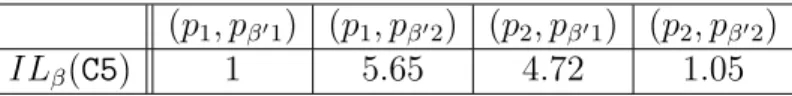
(p1, p 01) (p1, p 02) (p2, p 01) (p2, p 02)
IL (C5) 1 5.65 4.72 1.05
Table 5: Information leakage of program PROG C5
Example 5. Let’s consider again the parameters in Example 4. Since p 01 (resp. p 02), the slight modification of p 1 (resp. p 2), does not a↵ect the
adversary’s choice, it induces the same initial uncertainty as in Example 3. From Tables 2 and 4 we obtain the information leakage of the program PROG C5 as in Table 5.
We remark that when the initial belief and the actual a priori distribution are not highly conflicting (viz. (p1, p 01) and (p2, p 02)) the leakage is about 1
bit of information. Moreover, the leakage is almost equal to the actual leakage of the program. However, even though the leakage is high (more than 4 bits of information), when they are highly conflicting, the actual leakage cannot exceed two bits of information. Hence much of the leakage is due to the correction of the misinformation induced by the wrong belief.
We note that while the remaining uncertainty H1(A| O) is a good charac-terization of the vulnerability of A after observing O, the information leakage alone, as usual, does not tell us much about the security of A. Moreover it might correct a lot the misinformation induced by a wrong belief about A. It is therefore important to characterize the the amount of uncertainty induced by a wrong belief.
5.1. Accuracy
From Theorems 1 and 3 we learned that wrong beliefs increase uncer-tainty. We introduce here a metric for the accuracy of a belief which quanti-fies the amount of uncertainty induced by the belief inaccuracy. Intuitively, the more the belief is inaccurate, the more the adversary’s uncertainty should increase. We therefore quantify the inaccuracy of a belief by the divergence between the vulnerability induced by the belief and the actual vulnerability. Definition 8. The belief divergence of p and p (aka the inaccuracy of p w.r.t. p) is D (pk p ) = log⇣V (A)V (A)⌘.
D (pk p ) is always positive or null and accounts for the amount of in-crease in initial uncertainty due to the inaccuracy of p .
Lemma 1. D (pk p ) 0
Proof. Follows directly from Theorem 1.
Proposition 7. H1(A) = H1(A) + D (pk p )
Proof. Follows directly from their respective definitions (4 and 8).
Similarly we define the posterior inaccuracy as the divergence between the corresponding posterior vulnerabilities.
Definition 9. The posterior inaccuracy of p w.r.t. p is D (pk p : C) = log⇣V (AV (A| O)| O)⌘.
Again, it is always positive or null (cf. Theorem 3) and accounts for the amount of increase in the remaining uncertainty due to the inaccuracy of p . Lemma 2. D (pk p : C) 0
Proposition 8. H1(A| O) = H1(A| O) + D (p k p : C) 5.2. Leakage
In the previous section we have seen that a wrong belief increases the prior and the posterior min-entropy by the terms D (pk p ) and D (p k p : C), respectively. Note that D (pk p ) and D (p k p : C) can be arbitrary high. But: how do belief leakage and min-entropy leakage compare? We would expect the min-entropy leakage never to exceed the belief leakage, since the channel may correct the initial wrong belief and hence leaks more information. Actually this is not always the case. Indeed, as shown by our analysis of program PROG C2 (see Example 1) in Section 6, the belief leakage can be less, equal or greater than the min-entropy leakage. The reason is that the channel is not always reducing the inaccuracy of the belief. In fact a channel may increase the adversary’s confidence over some hypotheses which are actually very misleading. Thus the change in inaccuracy can be positive, null or even negative.
From Propositions 7 and 8 we have that a wrong belief increases (resp. decreases) the leakage by a term D (pk p : C) = D (p k p ) D (pk p : C) equal to the decrease (resp. increase) in inaccuracy. Hence, the belief leakage IL (p, C : p ) is related to the min-leakage IL1(p, C) as follows.
Proposition 9. IL (p, C : p ) = IL1(p, C) + D (pk p : C)
Interestingly, as in the case of the min-entropy leakage and the g-leakage, the belief leakage is also null when the low output and the high input are independent.
Theorem 5 (Zero-leakage). H1(A) H1(A| O) = 0 if A and O are inde-pendent.
Proof. Assume that A and O are independent. Then from Equation 9 we have that for all observable o, the posterior belief p (a| o) is equal to the prior belief p (a). Hence, o = for all observable o. In other words, the observables do not a↵ect the adversary’s choice. Therefore,
V (A| O) = X o2O p(o)V (A| o) =X o2O p(o)⇣ 1 | o| X a2 o p(a| o)⌘ = X o2O p(o)⇣ 1 | | X a2
p(a| o)⌘ ( Independence of A and O) = X o2O p(o)⇣ 1 | | X a2 p(a)⌘=X o2O
p(o)V (A) = V (A).
Hence H1(A| O) = H1(A).
Finally, we may wonder whether the belief leakage of a channel C can ever be negative, as C may increase the inaccuracy of a belief. However, as in the case of the min-entropy leakage and the g-leakage [25], the belief leakage is always positive or null as it is defined in terms of expectation. Theorem 6. H1(A) H1(A| O) 0.
6. On the Applicability of the Belief-vulnerability Approach
The previous section establishes our definitions in terms of their theo-retical properties. Now we show the utility of our approach by applying it to various threat scenarios and comparing the results to the previous ap-proaches. This is done through an extensive analysis of the deterministic program PROG C1 and the probabilistic program PROG C2 of Example 1. In order to simplify the reading, we reproduce them here.
PROG C2: BEGIN
R ‘sampled from {0, 2} with p(0) = and p(2) = 1 ’; If A = R Then O := A Else O := 1 END PROG C1: BEGIN O := b log(A + 2) c END
Each of these programs is analysed under the following hypothesis. • The actual prior distribution of the high input A is such that
p(a0) = p(a2) = !
2(1 + !) and p(a1) = p(a3) = 1 2(1 + !), for some 0 < ! 1.
• The adversary believes that A is most likely an even number, that is she assumes the following 12-admissible belief:
p (a0) = p (a2) = 3
8 and p (a1) = p (a3) = 1 8.
Thus ={a0, a2} and hence the probability that a guess of the attacker is correct is reduced by the factor ! compared to someone who knows the actual distribution.
We denote by IUx the initial uncertainty computed using the approach x 2 {s, 1, } where s, 1 and denote the Shannon entropy, R´enyi min-entropy and belief-based approaches respectively. Ditto for RUx and ILx. We start with PROG C1.
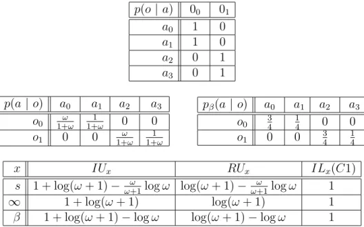
6.1. Analysis of PROG C1
Shannon entropy leakage. For the prior entropy we have: IUs = H(A) = X
a2A
p(a) log p(a)
= ⇣ ! 2(1 + !)log ! 2(1 + !) + 1 2(1 + !) log 1 2(1 + !) + ! 2(1 + !)log ! 2(1 + !) + 1 2(1 + !) log 1 2(1 + !) ⌘ = ⇣ ! 1 + ! log ! 2(1 + !) + 1 1 + ! log 1 2(1 + !) ⌘ = 1 + log(1 + !) ! 1 + ! log !.
For the posterior entropy, we have p(o0) = p(o1) = 12 since we have p(o) = P
a2Ap(o | a)p(a). The conditional probabilities p(a | o) =
p(o| a)p(a) p(o) are given in Table 6. Thus,
RUs = H(A| O) = X o2O
p(o)X a2A
p(a| o) log p(a | o) = h1 2 ⇣ ! 1 + !log ! 1 + ! + 1 1 + ! log 1 1 + ! ⌘ +1 2 ⇣ ! 1 + ! log ! 1 + ! + 1 1 + ! log 1 1 + ! ⌘i = ⇣ ! 1 + ! log ! 1 + ! + 1 1 + ! log 1 1 + ! ⌘ = log(1 + !) ! 1 + ! log !.
Hence the leakage is ILs = IUs RUs= 1. It is illustrated in Figure 1. Min-entropy leakage. For the prior min-entropy, we have
IU1 = H1(A) = log V (A) = log(max
a2A p(a)) = log 1 2(1 + !) = 1 + log(1 + !).
Similarly, for the posterior min-entropy, we have
RU1= H1(A| O) = log V (A| O) = log⇣X o2O p(o) max a2A p(a| o) ⌘ = log(1 2 · 1 1 + ! + 1 2 · 1 1 + !) = log(1 + !).
p(o | a) 00 01 a0 1 0 a1 1 0 a2 0 1 a3 0 1 p(a | o) a0 a1 a2 a3 o0 1+!! 1+!1 0 0 o1 0 0 1+!! 1+!1 p (a | o) a0 a1 a2 a3 o0 34 14 0 0 o1 0 0 34 14
x IUx RUx ILx(C1)
s 1 + log(! + 1) !+1! log ! log(! + 1) !+1! log ! 1 1 1 + log(! + 1) log(! + 1) 1 1 + log(! + 1) log ! log(! + 1) log ! 1
Table 6: Matrices of conditional probabilities and the leakages of PROG C1
Again, the leakage is 1 since IL1 = IU1 RU1 = 1. It is illustrated in Figure 1.
Belief leakage. Since the adversary initially believes that A is most likely even, then ={a0, a2}. Hence the belief vulnerability of A is
V (A) = 1 X a2 p(a) = 1 2 X a2{a0,a2} p(a)) = ! 2(1 + !).
Thus IU = H1(A) = log V (A) = 1 + log(1 + !) log(!).
For the posterior belief vulnerability, from Bayes’ rule, we obtain the ad-versary’s updated belief p (a| o) as in Table 6, whence we obtain the following sets of adversary’s possible choices o0 ={a0} and o1 ={a2}. Therefore,
V (A| O) = X o2O 1 | o| X a2 o p(o| a)p(a) = X j2{0,1} 1 | oj| X a2 oj p(oj| a)p(a) = p(o0| a0)p(a0) + p(o1| a2)p(a2) = !
1 + !.
Hence RU = H1(A| O) = log V (A| O) = log(1 + !) log(!), which results in a leakage of 1 again. Thus, the fact that the adversary initially
Figure 1: Shannon leakage of C1
Figure 2: Min-leakage of C1 Figure 3: Belief leakage of C1
believes that A is even does not a↵ect the quantity of information leaked by PROG C1. However, the real question is not how much information is leaked by this program, but what the remaining uncertainty represents in terms of security threat to the high input. Even though the adversary’s belief does not a↵ect the quantity of the information leakage, it dramatically a↵ects both the initial and remaining uncertainty. Indeed, as illustrated by Figure 3, both IU and RU tend toward infinity as ! tends toward zero. On the other hand, IU and RU tend toward two and one, respectively, as ! tends toward one. In other words inaccurate beliefs strengthen the security of the program (by confusing the adversary). Thus, a deliberate leakage of a wrong side information biased toward the less likely parity of the high input is a good strategy to strengthen the security of this program.
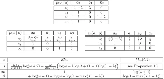
6.2. Analysis of PROG C2
We continue our analysis with the probabilistic program PROG C2. The initial uncertainty remains the same as in the analysis of the program PROG C1. Following the same approach as for PROG C1, we obtain the matrices of conditional probabilities and the leakages for PROG C2 shown in Table 7. Proposition 10 (Shannon entropy leakage of PROG C2).
ILs(C1) = 1 + log(! + 1) ! 2(! + 1)log ! ! + 2 2(! + 1)log(! + 2) + ! 2(! + 1) ⇣ log + (1 ) log(1 )⌘.
p(o| a) 00 01 02 a0 1 0 a1 1 0 0 a2 0 1 a3 1 0 0 p(a| o) a0 a1 a2 a3 o0 (12+!)! 2+!1 2+!! 2+!1 o1 1 0 0 0 o2 0 0 1 0 p (a| o) a0 a1 a2 a3 o0 35(1 ) 15 35 15 o1 1 0 0 0 o2 0 0 1 0 x RUx ILx(C2)
s 2(!+1)!+2 log(! + 2) 2(!+1)! ⇣log ! + log + (1 ) log(1 )⌘ see Propostion 10
1 1 log(! + 1)
1 + log(! + 1) log ! log(1 + max( , 1 )) log(1 + max( , 1 ))
Table 7: Matrices of conditional probabilities and the leakages of PROG C2
The information flow ascribed by the Shannon entropy is illustrated in Figures 4 and 5, those of the belief-based approach in Figures 6 and 7. We note that the randomisation parameter of PROG C2 has no e↵ect on the min-entropy leakage. This is due to the fact that this metric focuses on the single probability that poses the greatest risk; the actual posterior probabilities of a1 and a3, the possible choices of the adversary, do not depend on . On the other hand, the accuracy factor ! of the adversary’s prior belief has no e↵ect on the belief leakage. This is due to the fact that she always chooses the even number a0 or a2 towards which is biased independently of !. Since a0 and a2 play symmetric roles with respect to , any gain in uncertainty due to the value towards which is biased is o↵set by the loss due to the other value.
Finally, comparing the min-entropy leakage and the belief leakage of PROG C2(see Figure 8), we can assert that belief leakage is higher than min-entropy leakage except for highly accurate beliefs. In fact, we have the following result relating min-entropy and belief leakages depending on the randomisation parameter and !, the accuracy factor of the adversary’s prior belief. Proposition 11. The belief leakage of PROG C2 is higher than its min-entropy leakage if and only if the randomisation parameter and !, the accuracy factor of the adversary’s prior belief, satisfy the following relation:
Figure 4: RUsof PROG C2 Figure 5: ILs of PROG C2
Figure 6: RU of PROG C2 Figure 7: IL of PROG C2
6.3. Belief accuracy vs adversary’s confidence
Our analysis so far confirmed that inaccurate beliefs tend to confuse the adversary by reducing the probability that she correctly guesses the hidden or protected data. However, it might be the case that the interaction with the security mechanism (wrongly) increased the adversary’s confidence about the value of the hidden or protected data, that is, she wrongly believes that she has learned some useful information. Hence, she may end up being highly confident about her (wrong) result and may take action that results in serious harm to an innocent victim or to the whole society.
For instance, assume thatA is the set of hidden identities of the users of the security system. Consider a ‘dictator’ adversary who takes action against a user a only when she believes that a is more likely to be the culprit (i.e.
Figure 8: Belief leakage vs min-entropy leakage (PROG C2)
more likely to be the hidden input) than to not be the culprit. In other words, she only takes action against a when p (a) > 12 a priori or p (a| o) > 12 a posteriori for a given observable o.
Now let us see how our simple programs C1 and C2 perform against such adversary. First, we note that, a priori, there is no victim since the adver-sary’s prior belief p does not assign a mass strictly higher than one-half to any value of A. However, after observing the outcome of C1 (see Table 6) we have that ˜p (a0 | o0) = ˜p (a2 | o1) = 34. Therefore, the adversary will take action against a0 (resp. a2) when she observes o0 (resp. o1) even though a0 (resp. a2) is highly unlikely to be the input when !, the accuracy factor of the adversary’s prior belief, is very small. Let P rob[Vic : p , p, C] (resp. P rob[Inn : p , p, C]) denote the probability that the adversary takes action against a user (resp. an innocent user) after observing the outcome of the channel C when her prior belief is p and the actual prior probability is p. Let p and p be as in the previous section. Then the followings hold.
as follows. P rob[Vic : p , p, C1] = 1 P rob[Inn : p , p, C1] = 1 1 + ! P rob[Vic : p , p, C2] = ⇢ ! 2(1+!) if 1 6 5 6 1 otherwise P rob[Inn : p , p, C2] = ( 0 if 16 5 6 2+!⇥min( ,1 ) 2(1+!) otherwise
Proof. The probability of having a victim can be expressed as the sum of the probability P rob[p (a| o) > 1
2] that user a is a victim given the observable o weighted by the actual probability p(o) of the observable. Hence
P rob[Vic : p , p, C] =X o2O X a2A p(o)⇥ P rob[p (a | o) > 1 2].
Similarly, the probability of having an innocent victim can be expressed as the sum of the probability of having a victim a for each observable o weighted by the actual probabilityPa06=ap(a0| o) that somebody else could have been
the actual input. Thus
P rob[Vic : p , p, C] = X o2O X a2A p(o)⇥ P rob[p (a | o) > 1 2] ⇣X a06=a p(a0| o)⌘. Since p(o) = Pa2Ap(o| a)p(a), the proposition follows from Table 6 and Table 7.
The results above show that in terms of protecting everybody (i.e. not having victims), C1 ensures zero level of protection, since whatever the out-come of the program is the adversary will beout-come confident enough about her guess to take action. Ditto for C2 when the randomization factor is highly biased towards one value of A. However, when is not highly biased, then C2 becomes extremely good, since the most likely outcome o0 does not in-crease the adversary’s confidence enough to trigger an action, specially when !, the accuracy factor of her prior belief, is very small. Hence in terms of protecting everybody against such ‘dictator’ adversary, C2 performs better than C1 when is not highly biased. But they are equally bad when is highly biased.
In terms of protecting only the innocent victims, C2 is perfect when is not highly biased, since in this case the adversary will never take action against an innocent victim. However when is highly biased, C2 becomes slightly worse that C1. The reason is that in this case even when the input is an even number there is a small probability that the adversary’s guess is wrong for C2 when she observes o0. This is never the case for C1.
The elementary examples in this paper illustrate the applicability of our metric to various threat scenarios. In particular, they show that confidence, i.e., the entropy of the adversary’s belief, and accuracy are two orthogonal dimensions of security. We need to consider both of them in order to be able to model a wide range of threat scenarios. Typically, the adversary makes her decision according to her confidence in her beliefs, i.e., based on the uncertainty metric. On the other hand, the consequence of her decision, viz., the gain, usually depends on the accuracy metric. The ‘dictator’ example illustrates the limit case where the gain is independent of the accuracy (as the dictator always wins). It also shows the importance of the reliability of side information.
7. Related work
We have already mentioned in Sections 1 and 3 much of the related work. In this section we only discuss the work that is closely related to our frame-work and that was not already reported there.
As far as we know, [21, 22] have been the first papers to address the adversary’s beliefs in quantifying information flow. This line of work, which inspired our formulation of the belief-vulnerability, is based on the Kullback-Leibler distance, a concept related to Shannon entropy which in general, as already mentioned in Section 3, fails to characterize many realistic attacks scenarios. Belief semantics has been explored also in the context of other security properties in [39, 40]. In a recent paper [41], Hussein proposed a generalization of the Bayesian-based framework of [22] based on Dempster-Shafer theory. The accuracy is expressed in terms of the generalized Jensen-Shannon divergence [42] between the belief and the actual value of the high input. Our metric is, on the contrary, based on the min-entropy leakage, where a leakage of k-bits means that on average the channel increases the vulnerability of the secret to being guessed correctly in one single try by the factor 2k. Moreover, as shown by recent work [25], quantitative information flow metrics based on the min-entropy model can be extended by so-called
gain functions to account for a wider range of operational attack scenarios. While the framework in [25] is closely related to ours, as they both generalize the quantitative information flow model based on R´enyi min-entropy, their objectives are orthogonal. Belief functions model the adversary’s (potentially incorrect) side information; gain-functions model the operational threat sce-narios, such as the adversary’s benefit from guessing a value ‘close’ to the actual value of the secret, guessing a property of the secret, or guessing its value within some number of tries.
A related line of research has explored methods of statistical inference, in particular those from the hypothesis testing framework. The idea is that the adversary’s best guess is that the true input is the one which has the maxi-mum conditional probability (MAP rule) and that, therefore, the a posteriori vulnerability of the system is the complement of the Bayes Risk, which is the average probability of making the wrong guess when using the MAP rule [43]. This is always at least as high as the a priori vulnerability, which is the probability of making the right guess just based on the knowledge of the input distribution. It turns out that Smith’s notion of leakage actually cor-responds to the ratio between the a posteriori and the a priori vulnerabilities [24, 44].
Concerning the computation of the channel matrix and of the leakage for probabilistic systems, one of the first works to attack the problem was [45], in which the authors proposed various model-checking techniques. One of these is able to generate counterexamples, namely points in the execution where the channel exhibits an excessive amount of leakage. This method is therefore also useful to fix unsound protocols. A subsequent paper [46] focussed more on the efficiency and proposed the use of binary decision di-agrams and symbolic model checking. For systems that are too large to apply model-checking, approximate techniques based on statistics have been proposed [47].
8. Conclusion and future work
This paper presents a new approach to quantitative information flow that incorporates the attacker’s beliefs in the model on R´enyi min entropy. We investigate the impact of such adversary’s inaccurate, misleading or outdated side information on the security of the secret information. Our analysis reveals that inaccurate side information tends to confuse the adversary by decreasing the probability of a correct guess. However, due to the inaccuracy
of her side information, the interaction with the security mechanism may (wrongly) strengthen the adversary’s confidence about her choice. While the attacker might not actually discover the true value of the secret, the fact that she wrongly believes to actually know it constitutes a security threat, since it can adversely influence how she views or interacts with the victim. We have shown the strength of our definitions both in terms of their theoretical properties and of their utility by applying them to various threat scenarios. As already stated in [21, 22], our results confirm, in particular, that the confidence of the attacker and the accuracy of her belief are two orthogonal dimensions of the security. Depending on the threat operational scenario, both could be equally important or one more relevant than the other. We observe that our approach can also be seen as moving away from the often criticised yet standard assumption in information flow that the adversary knows the true distribution of secrets. More realistically, here the focus is on the attacker’s assumptions about such distributions (their a priori beliefs), and the consequences of making them.
As future work, we shall extend our model to consider a wide range of operational threat scenarios especially in the presence of wrong beliefs. To achieve this goal, we plan to build upon our belief framework and the gain-functions framework [25]. Secondly, we shall devise methods and techniques of collecting and aggregating the adversary’s side information from di↵erent and potentially conflicting sources such as social networks, online forums and blogs, etc. We believe that the body of concepts and results related to the notion of belief combination will provide natural and solid tools for this goal. Finally, we also plan to implement our framework in a tool to assess the e↵ectiveness of current security/privacy mechanisms in a real-world context and under various attack scenarios. Doing so, will help us to have a clear view of the real impact of side information collected from social networks, online forums, blogs and other forms of online communication and information sharing. It will also help us to accurately estimate the reliability of each of these sources, as well as providing guidelines and some mechanism design principles for privacy-preserving and security mechanisms.
[1] D. Chaum, The dining cryptographers problem: Unconditional sender and recipient untraceability, Journal of Cryptology 1 (1988) 65–75. [2] M. K. Reiter, A. D. Rubin, Crowds: anonymity for Web transactions,
ACM Transactions on Information and System Security 1 (1) (1998) 66–92.
[3] P. Syverson, D. Goldschlag, M. Reed, Anonymous connections and onion routing, in: IEEE Symposium on Security and Privacy, Oakland, Cali-fornia, 1997, pp. 44–54.
[4] I. Clarke, O. Sandberg, B. Wiley, T. W. Hong, Freenet: A distributed anonymous information storage and retrieval system., in: Designing Pri-vacy Enhancing Technologies, International Workshop on Design Issues in Anonymity and Unobservability, Vol. 2009 of Lecture Notes in Com-puter Science, Springer, 2000, pp. 44–66.
[5] P. F. Syverson, S. G. Stubblebine, Group principals and the formaliza-tion of anonymity, in: World Congress on Formal Methods (1), 1999, pp. 814–833.
[6] J. Y. Halpern, K. R. O’Neill, Anonymity and information hiding in multiagent systems, Journal of Computer Security 13 (3) (2005) 483– 512.
[7] D. Hughes, V. Shmatikov, Information hiding, anonymity and privacy: a modular approach, Journal of Computer Security 12 (1) (2004) 3–36. [8] S. Schneider, A. Sidiropoulos, CSP and anonymity, in: Proc. of the European Symposium on Research in Computer Security (ESORICS), Vol. 1146 of LNCS, Springer, 1996, pp. 198–218.
[9] P. Y. Ryan, S. Schneider, Modelling and Analysis of Security Protocols, Addison-Wesley, 2001.
[10] M. Bhargava, C. Palamidessi, Probabilistic anonymity, in: M. Abadi, L. de Alfaro (Eds.), Proceedings of CONCUR, Vol. 3653 of Lecture Notes in Computer Science, Springer, 2005, pp. 171–185.
[11] K. Chatzikokolakis, C. Palamidessi, Probable innocence revisited, The-oretical Computer Science 367 (1-2) (2006) 123–138, http://www.lix. polytechnique.fr/~catuscia/papers/Anonymity/tcsPI.pdf.
URL http://hal.inria.fr/inria-00201072/en/
[12] T. M. Cover, J. A. Thomas, Elements of Information Theory (Wiley Se-ries in Telecommunications and Signal Processing), Wiley-Interscience, 2006.
[13] Y. Zhu, R. Bettati, Anonymity vs. information leakage in anonymity systems, in: Proc. of ICDCS, IEEE Computer Society, 2005, pp. 514– 524.
[14] D. Clark, S. Hunt, P. Malacaria, Quantitative information flow, relations and polymorphic types, Journal of Logic and Computation, Special Issue on Lambda-calculus, type theory and natural language 18 (2) (2005) 181–199.
[15] P. Malacaria, Assessing security threats of looping constructs, in: M. Hofmann, M. Felleisen (Eds.), Proceedings of the 34th ACM SIGPLAN-SIGACT Symposium on Principles of Programming Lan-guages, POPL 2007, Nice, France, January 17-19, 2007, ACM, 2007, pp. 225–235.
URL http://doi.acm.org/10.1145/1190216.1190251
[16] P. Malacaria, H. Chen, Lagrange multipliers and maximum informa-tion leakage in di↵erent observainforma-tional models, in: ´Ulfar Erlingsson and Marco Pistoia (Ed.), Proceedings of the 2008 Workshop on Program-ming Languages and Analysis for Security (PLAS 2008), ACM, Tucson, AZ, USA, 2008, pp. 135–146.
[17] I. S. Moskowitz, R. E. Newman, P. F. Syverson, Quasi-anonymous chan-nels, in: IASTED CNIS, 2003, pp. 126–131.
[18] I. S. Moskowitz, R. E. Newman, D. P. Crepeau, A. R. Miller, Covert channels and anonymizing networks., in: S. Jajodia, P. Samarati, P. F. Syverson (Eds.), WPES, ACM, 2003, pp. 79–88.
[19] K. Chatzikokolakis, C. Palamidessi, P. Panangaden, Anonymity proto-cols as noisy channels, Information and Computation 206 (2–4) (2008) 378–401. doi:10.1016/j.ic.2007.07.003.
URL http://hal.inria.fr/inria-00349225/en/
[20] M. Franz, B. Meyer, A. Pashalidis, Attacking unlinkability: The im-portance of context, in: N. Borisov, P. Golle (Eds.), Privacy Enhancing Technologies, 7th International Symposium, PET 2007 Ottawa, Canada, June 20-22, 2007, Revised Selected Papers, Vol. 4776 of Lecture Notes in Computer Science, Springer, 2007, pp. 1–16.
[21] M. R. Clarkson, A. C. Myers, F. B. Schneider, Belief in information flow, in: CSFW, IEEE Computer Society, 2005, pp. 31–45.
[22] M. R. Clarkson, A. C. Myers, F. B. Schneider, Quantifying information flow with beliefs, Journal of Computer Security 17 (5) (2009) 655–701. [23] G. Smith, Adversaries and information leaks (tutorial), in: G. Barthe,
C. Fournet (Eds.), Proceedings of the Third Symposium on Trustworthy Global Computing, Vol. 4912 of Lecture Notes in Computer Science, Springer, 2007, pp. 383–400.
URL http://dx.doi.org/10.1007/978-3-540-78663-4_25
[24] G. Smith, On the foundations of quantitative information flow, in: L. De Alfaro (Ed.), Proceedings of the Twelfth International Conference on Foundations of Software Science and Computation Structures (FOS-SACS 2009), Vol. 5504 of Lecture Notes in Computer Science, Springer, York, UK, 2009, pp. 288–302.
[25] M. S. Alvim, K. Chatzikokolakis, C. Palamidessi, G. Smith, Measuring information leakage using generalized gain func-tions, in: Proceedings of the 25th IEEE Computer Se-curity Foundations Symposium (CSF), 2012, pp. 265–279. doi:http://doi.ieeecomputersociety.org/10.1109/CSF.2012.26.
[26] A. McIver, C. Morgan, G. Smith, B. Espinoza, L. Meinicke, Abstract channels and their robust information-leakage ordering, in: M. Abadi, S. Kremer (Eds.), Proceedings of the Third International Conference on Principles of Security and Trust (POST), Vol. 8414 of Lecture Notes in Computer Science, Springer, 2014, pp. 83–102.
[27] M. S. Alvim, K. Chatzikokolakis, A. McIver, C. Morgan, C. Palamidessi, G. Smith, Additive and multiplicative notions of leakage, and their ca-pacities, in: IEEE 27th Computer Security Foundations Symposium, CSF 2014, Vienna, Austria, 19-22 July, 2014, IEEE, 2014, pp. 308–322. doi:10.1109/CSF.2014.29.
[28] S. Hamadou, C. Palamidessi, V. Sassone, E. ElSalamouny, Probable innocence in the presence of independent knowledge, in: P. Degano, J. D. Guttman (Eds.), Formal Aspects in Security and Trust, FAST