Nonlinear Control of Mechanical Systems with an Unactuated Cyclic Variable

HAL Id: hal-00794882

https://hal.archives-ouvertes.fr/hal-00794882

Submitted on 26 Feb 2013

HAL is a multi-disciplinary open access

archive for the deposit and dissemination of

sci-entific research documents, whether they are

pub-lished or not. The documents may come from

teaching and research institutions in France or

abroad, or from public or private research centers.

L’archive ouverte pluridisciplinaire HAL, est

destinée au dépôt et à la diffusion de documents

scientifiques de niveau recherche, publiés ou non,

émanant des établissements d’enseignement et de

recherche français ou étrangers, des laboratoires

publics ou privés.

Unactuated Cyclic Variable

Jessy Grizzle, Claude Moog, Christine Chevallereau

To cite this version:

Jessy Grizzle, Claude Moog, Christine Chevallereau. Nonlinear Control of Mechanical Systems with

an Unactuated Cyclic Variable. IEEE Transactions on Automatic Control, Institute of Electrical and

Electronics Engineers, 2005, 50 (5), pp.559 - 576. �hal-00794882�

Nonlinear Control of Mechanical Systems with an

Unactuated Cyclic Variable

J.W. Grizzle, Fellow, IEEE, C.H. Moog, Senior Member, IEEE, and C. Chevallereau

Abstract— Numerous robotic tasks associated with

underactu-ation have been studied in the literature. For a large number of these in the plane, the mechanical models have a cyclic variable, the cyclic variable is unactuated, and all shape variables are independently actuated. This paper formulates and solves two control problems for this class of models. If the generalized momentum conjugate to the cyclic variable is not conserved, conditions are found for the existence of a set of outputs that yields a system with a one-dimensional exponentially stable zero dynamics — i.e. an exponentially minimum-phase system — along with a dynamic extension that renders the system locally input-output decouplable. If the generalized momentum conjugate to the cyclic variable is conserved, a reduced system is constructed and conditions are found for the existence of a set of outputs that yields an empty zero dynamics, along with a dynamic extension that renders the system feedback linearizable. A common element in these two feedback problems is the construction of a scalar function of the configuration variables that has relative degree three with respect to one of the input components. The function arises by partially integrating the conjugate momentum. The results are illustrated on two balancing tasks and on a ballistic flip motion.

I. INTRODUCTION

Underactuated mechanical systems have fewer actuators than degrees of freedom. Underactuation is naturally associ-ated with dexterity. For example, the act of standing with one foot flat on the ground is not viewed as particulary dexterous, whereas a headstand or sur les pointes (ballet) are considered dexterous. In the first case, since the foot is not in rotation with respect to the ground, the point of rotation is the ankle, which is actuated, as are each of the joints further up the tree; that is to say, normal standing involves a fully actuated system. On the other hand, in headstands or when on pointe, the contact point between the body and ground is acting as a pivot without actuation. These are underactuated systems. In these examples, a typical control task would be to hold an equilibrium pose with (asymptotic) stability, or to execute a motion (e.g., a relev´e lent, battement) without falling over (i.e., with internally bounded states).

Motions that include a ballistic phase are also often viewed as dexterous. Examples include dismounting from a high bar or platform diving. In these cases, the underactuation is manifest in the lack of contact with any surface. The ballistic phase is

Manuscript received 03 November, 2003; revised 25 August, 2004. Jessy W. Grizzle is with the Control Systems Laboratory, Electrical Engineering and Computer Science Department, University of Michigan, Ann Arbor, MI 48109-2122, USA,grizzle@umich.edu.

Claude H. Moog and Christine Chevallereau are with IRCCyN, Ecole Cen-trale de Nantes, UMR CNRS 6597, BP 92101, 1 rue de la No¨e, 44321 Nantes cedex 03, France,{Claude.Moog, Christine.Chevallereau}

@irccyn.ec-nantes.fr

normally of short duration since reestablishing contact with a surface (e.g., ground, mat, water, ...) is an objective of the maneuver. A typical control problem would be to execute a predefined motion, with emphasis on achieving a final state that is compatible with an elegant landing on a mat (no rebounding or slipping), or re-entry into the water (no splash). Similar things can be said for back flips, tumbling, and somersaults.

The objective of this paper is to contribute to the control of mechanical systems that are capable of executing such dexterous maneuvers in the plane. The literature on underactu-ated (a.k.a. super-articulunderactu-ated [50]) systems and nonholonomic systems is vast. A few representative control works include the study of accessibility in [44], stabilization of equilibria through passivity techniques in [40] and energy shaping in [3], stabilization and tracking via backstepping in [24, 25, 50], the use of virtual constraints to achieve stabilization of orbits in [51], and path planning in [4]. Representative works in the robotics area are cited in Section II. One of the novelties of the present paper is to recognize that balancing on a pivot while executing a motion and planning a back flip share a common mathematical problem: designing a set of outputs that result in a minimal zero dynamics: exponentially minimum phase and one dimensional in the first case, and empty, in the second. In part, this is of course related to the maximal feedback linearization problem, which has been solved completely when static state feedback is considered [31], while only partial results are known when dynamic state feedback is allowed,

c.f. [12, 29] and references therein. The additional requirement

being achieved here is that the “non-feedback linearizable part” of the system is exponentially stable, and no general results are available on this aspect.

Section II identifies a special class of mechanical systems with one degree of underactuation that underlies the study of dexterous maneuvers in the plane as discussed previously. The key feature is that the systems possess a cyclic variable and this variable is unactuated [38]. Section III formulates and solves two related control problems. If the generalized momentum conjugate to the cyclic variable is not conserved, conditions are found for the existence of a set of outputs that yields an exponentially minimum phase system with a one-dimensional zero dynamics, along with a dynamic extension that renders the system locally input-output decouplable. When these two properties are met, it is well known that asymptotic tracking of an open set of output trajectories is possible, with all internal states remaining bounded [22]. If the generalized momentum conjugate to the cyclic variable is conserved, a reduced system is constructed and conditions are found for the existence of

a set of outputs that yields an empty zero dynamics, along with a dynamic extension that renders the system input-output decouplable. When these two properties are met, is well known that local dynamic state feedback linearization is possible [22].

In both of these feedback problems, the principal contribution is the construction of a scalar function of the configuration variables that has relative degree three with respect to one of the input components [5]. The theoretical results are illustrated

on three simple examples in Section IV. The paper is wrapped up with some additional discussion of the results in Section V and concluding remarks in Section VI.

II. MOTIVATINGCLASSES OFSYSTEMS

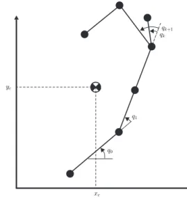
This section uses two classes of systems to set the stage for the mathematical and control developments that follow. The first class consists of_{N ≥ 2 planar rigid bodies connected in} a tree structure—no closed kinematic chains—with the base attached to an inertial reference frame via a pivot, that is, an unactuated revolute joint. It is supposed that each link has nonzero mass, and that each connection of two links is independently actuated so that the system has one degree of underactuation (_{N degrees of freedom with N −1 independent} actuators). It is further supposed that all joints are frictionless, but this assumption is really only important at the pivot. Figure 1 shows an example of such a system. Though not indicated in the figure, massless springs may be attached between links and between links and the inertial reference frame; prismatic joints between links are also allowed. This class of systems clearly includes the Acrobot [2, 36, 52], the brachiating robots of [15, 34, 35, 46], the gymnast robots of [32, 39, 57] when pivoting on a high bar, and the stance phase models of Raibert’s one-legged hopper [1, 6, 14, 26, 33, 42] as well as RABBIT [7–10, 41]. The control objectives will be to stabilize the system about an equilibrium point or to track a set of reference trajectories with internal stability. The second class of systems consists of _{N ≥ 2 planar rigid bodies, once again connected in a tree} structure, but this time, it is assumed that the mechanism is undergoing ballistic motion. As before, it is supposed that that each link has nonzero mass and each connection of two links is independently actuated. In addition, it is assumed that there are no springs between any link and an inertial reference frame. Such a system has three degrees of underactuation: N + 2

degrees of freedom and _{N − 1 independent actuators. Figure} 2 shows an example of such a system. This class of systems clearly includes the gymnast robot of [32] when dismounting from the high bar, the planar diver of [17], the flip gait of the robot in [16], the ballistic phase of the 4-link planar robot in [47], and the ballistic phase of running in planar biped robots [8] and Raibert’s hopper [1, 6, 14, 26, 42]. The control objective will be to maximally linearize the system so as to facilitate the construction of a trajectory that transfers the state of the system from one point to another in finite time.

Consider the N -link system shown in Figure 1, along with

the indicated coordinates,q = (q0, q1, · · · , qN −1), where, for

convenience, the reference frame has been attached at the pivot point. The kinetic energy is quadratic, K = 1₂˙qT_{D(q) ˙q, with}

D positive definite. Since the kinetic energy is independent

q0

q1

qk

qk+1

Fig. 1. A planar tree structure attached to an inertial frame via a freely acting pivot. All joints are actuated except the attachment at the pivot. A coordinate convention is indicated. Though not shown, prismatic joints and springs can also be included. q0 q1 qk qk+1 xc yc

Fig. 2. A planar tree structure in ballistic motion. All joints are actuated. A coordinate convention is indicated. Though not shown, prismatic joints can be included as can springs that act between links but not between a link and the inertial frame.

of the orientation of the reference frame,D is independent of q0; that is ∂D(q)_∂q0 ≡ 0. The coordinate q0 is said to be cyclic

[18] (a.k.a. external in [37]) whereas(q1, ..., qN −1) are called

shape variables. The form of the potential energyV depends

on whether the system is evolving under the action of gravity (for example, in a vertical plane versus a horizontal plane) and whether or not springs have been attached at the joints. Electromagnetic and electrostatic forces are excluded, and hence, the potential energy depends only on the configuration variables. Mechanical systems where the kinetic energy is quadratic in the velocities and the potential energy depends only on the configuration variables are said to be simple.

Denote the Lagrangian by_{L = K − V , and assume that the} system is actuated such that

d dt ∂L ∂ ˙qk − ∂L ∂qk = ½ 0 k = 0 uk k = 1, · · · , N − 1 , (1)

withuk taking values in IR. The model thus takes the form D(q)¨q + C(q, ˙q) ˙q + G(q) = Bu, (2) where B = · 0 I ¸ .

Consider next the N -link system shown in Figure 2, along

with the indicated coordinates,qe= (q, xc, yc), where (xc, yc)

are the Cartesian coordinates of the center of mass. Suppose further that there are no springs between a link and an inertial reference frame. Then the equations of motion decompose as

¯ D(q)¨q + ¯C(q, ˙q) ˙q + ¯G(q) = Bu ¨ xc = 0 ¨ yc = g0, (3)

where in a vertical planeg0is the gravitational constant and if

the system is evolving on a horizontal plane without friction, then g0 = 0. As in the first class of systems considered, q0

is also a cyclic variable of ¯D because the kinetic energy is

independent of the chosen orientation of the inertial reference frame.

The important point is that the dynamics of the body coordinates, q, and the Cartesian coordinates of the center

of mass, (xc, yc), are decoupled. Since the center of mass

coordinates are unactuated, the control of the system (3) can be reduced to the control of a system having one degree of underactuation as in (2) by eliminating the trivial dynamics

¨

xc = 0, ¨yc = g0. In this sense, the two systems in Figures 1

and 2 are very similar: they give rise to control problems for systems with _{N ≥ 2 DOF, (N − 1) actuators, and the cyclic} coordinate is unactuated. One way in which the systems are often different is that angular momentum about the center of mass of (3) is always conserved, whereas (2) may or may not have a conserved quantity depending on the potential energy. For example, consider a system as in Figure 1 in a horizontal plane without friction; suppose furthermore there are no springs between any link and the inertial reference frame. Then the angular momentum about the pivot point is a conserved quantity, and thus this feature—conservation of angular momentum—is possible in (2) as well. Conservation of angular momentum gives rise to a nonholonomic constraint [27] and changes fundamentally the nature of the control problem.

In summary, the models of the simple mechanical systems represented by Figures 1 and 2 present the common feature of an unactuated, cyclic variable. The system (2) has one degree of underactuation whereas even though the system (3) has three degrees of underactuation, in the proper coordinates, the control problem decouples into the control of a system of the form (2) plus keeping track of the evolution of the center of mass variables. These observations are used in the next section to motivate the class of models analyzed. As a final remark, it is worth noting that [38] has shown quite clearly that even for systems with two degrees of freedom, if the cyclic coordinate and the unactuated coordinate do not coincide—such as in the inverted pendulum on a cart—then the system possesses quite different properties from a control point of view.

III. CONTROL OFSIMPLEMECHANICALSYSTEMS WITH ANUNACTUATEDCYCLICVARIABLE

Consider the classes of mechanical systems motivated in Section II. Roughly speaking, the goal is to determine a set of outputs that gives rise to a zero dynamics of “smallest possible” dimension, and if this dimension is non-zero, also to assure that the zero dynamics is stable [5]. More precisely, in the case of a system where the generalized momentum conjugate to the cyclic variable is not conserved, a set of outputs will be found that leads to local dynamic input-output decouplability and a one-dimensional exponentially stable zero dynamics, and for systems where the conjugate momentum is conserved, a set of flat outputs [13, 45] will be determined; that is, a set of outputs will be found that leads to the construction of a regular dynamic feedback and a local change of coordinates in which the system is linear.

Before proceeding, it is worth noting that if outputs are chosen to correspond to the actuated variables, that is,yi= qi

, for _{i = 1, · · · , N − 1, then each component has relative} degree two and the associated decoupling matrix is invertible (one says the system has vector relative degree _{(2, · · · , 2)} [22]). Such a choice leads to a two-dimensional zero dynamics, which, moreover, can be shown to be once again a Lagrangian system [56], and thus can never have an asymptotically stable equilibrium. One way to get around this problem is to construct a set of outputs such that the associated zero dynamics has dimension one, and hence is not Lagrangian. For special cases, [5] shows how to construct an output component that has relative degree three with respect to one of the input components. This idea is developed in much more generality here.

A. Partial integration of a one-form

This subsection presents a key result that will lead to the construction of outputs for the system (2) so that the associated zero dynamics has dimension one, and hence may admit an asymptotically stable equilibrium point. As will be seen in the next subsection, the abstract one-form considered here naturally arises from consideration of momentum. The result formalizes and extends previous work of [5] and [38].

The following lemma can be viewed as a special case of the Pfaff-Darboux Theorem, whose role in control systems theory was first highlighted in [21]. As a point of notation, given a collection of smooth real-valued functions _{fi|1 ≤ i ≤ k}

defined on some open set _{O, span {df}i|1 ≤ i ≤ k} denotes

the corresponding codistribution as defined in [22]; that is, the span is computed point-wise overIR.

Lemma 1: Consider a smooth N-dimensional manifoldQ.

Let_{ω ∈ T}∗_{Q be a smooth one-form on Q and suppose there}

is a set of coordinates (q0, q1, · · · , qN −1) defined in an open

neighborhood_{O of a point (q}∗ 0, q∗1· · · , qN −1∗ ) in which ω has the form ω = dq0+ N −1 X k=1 αk(q1, · · · , qN −1)dqk. (4)

Then for any_{1 ≤ m ≤ N − 1, there exists a smooth function}

pm: O → IR such that at each point of O

ω = dpm mod span {dqi|1 ≤ i ≤ N − 1, i 6= m} . (5)

Moreover, in the coordinates (q0, q1, · · · , qN −1), one such

function is pm= q0−q∗0+ Z qm q∗ m αm(q1, · · · , qm−1, τ, qm+1, · · · , qN −1)dτ. (6)

Proof: Becauseω is smooth, the functions αkare smooth

on _{O. The integral in (6) is well-defined at each point in O} because the integrand is smooth and the integral is evaluated over a closed and bounded interval. Since

dpm= dq0+ αm(q1, · · · , qN −1)dqm+ N −1 X k=1,k6=m Z qm q∗ m ∂αm(q1, · · · , qm−1, τ, qm+1, · · · , qN −1) ∂qk dτ dqk,

it follows immediately that, at each point in_O,

ω − dpm∈ span {dqi|1 ≤ i ≤ N − 1, i 6= m} . (7)

Remark 1: TheN -tuple (pm, q1, · · · , qN −1) is a valid set

of coordinates on_{O. Indeed,} q0= q0∗+pm− Z qm q∗ m αm(q1, · · · , qm−1, τ, qm+1, · · · , qN −1)dτ.

Said another way, the map that takes (q0, q1, · · · , qN −1) to

(pm, q1, · · · , qN −1) is a diffeomorphism. Note that if O is all

of Q, then the result of Lemma 1 is global.

B. Model class and a normal form

Consider a simple1 _{N ≥ 2 DOF Lagrangian system with}

N − 1 independent actuators, where the unactuated variable is

a cyclic coordinate of the kinetic energy. Specifically, let the configuration space be Q, an open connected subset of IRN_,

with local coordinates denoted by q = (q0, q1, · · · , qN −1),

and take canonical coordinates (q, ˙q) on T Q. Let the kinetic

energy be given by K = 1₂˙qT_{D(q) ˙q, where D is positive}

definite and smooth everywhere onQ, and satisfies ∂D(q)_∂q0 ≡ 0

(i.e., q0 is cyclic). Let the potential energy, V, depend only

on the configuration variables and be smooth. Denote the Lagrangian by _{L = K − V and assume that the system is} actuated according to (1). The model can then be written as in (2). Subsequent analysis and feedback design are more easily accomplished if the system is first transformed into the normal form [44, 53] ¨ q0 = PN −1k=1 Jk(q1, · · · , qN −1)vk+ R(q, ˙q) ¨ q1 = v1 .. . ¨ qN −1 = vN −1, (8)

where Jk = −d_d0,k0,0, d0,k,k = 0, · · · , N − 1 are the entries in

the first row of D. The definition of R(q, ˙q) and the required

1_{Recall that simple means that the kinetic energy is quadratic in the}

velocities and the potential energy depends only on the configuration variables.

(regular) static state feedback transformation are given in the Appendix. Note that everywhereD is positive definite, d0,0 is

never zero. Note also thatJk does not depend on q0 because

q0 is cyclic.

Denote the generalized momentum conjugate toq0 [18] by

σ = _∂∂L_q˙0. Because the kinetic energy is quadratic and the

potential energy depends only on the configuration variables, it follows that σ = N −1 X k=0 d0,k(q1, · · · , qN −1) ˙qk. (9)

From the assumption on the actuation and the assumption that

q0 is cyclic,

˙σ = −_∂q∂V

0(q).

(10) For later use, note that (10) implies that the relative degree of

σ is at least three2_{. Using (9) and (10) to express the normal}

form in terms of the state variablesq0, q1, . . . , qN, σ, ˙q1. . . ˙qN,

instead ofq0, · · · , qN, ˙q0, · · · , ˙qN, shows that (2) is (globally)

static state feedback equivalent to

˙q0 = _d0 σ ,0(q1,··· ,q_{N −1})+ PN −1 k=1 Jk(q1, · · · , qN −1) ˙qk ˙σ = −∂V ∂q0(q) ¨ qj = vj, j = 1, · · · , N − 1, (11) which was introduced in [37] and will be called the modified normal form. Since only a change of state variables has been made, the feedback required to go from (2) to (11) is the same as that used in (8).

Associate toσ the one-form ˜ ω = N −1 X k=0 d0,k(q1, · · · , qN −1)dqk,

and the normalized one-form

ω = dq0+ N −1 X k=1 d0,k d0,0 (q1, · · · , qN −1)dqk.

Applying Lemma 1 form = 1, define the function p1= q0− q0∗+ Z q1 q∗ 1 d0,1 d0,0 (τ, q2, · · · , qN −1)dτ. (12)

Direct computation then leads to

dp1 dt = σ d0,0(q1, · · · , qN −1) + N −1 X k=2 βk(q1, · · · , qN −1) ˙qk, (13) where, βk(q1, · · · , qN −1) = Rq 1 q∗ 1 ∂ ∂qk d0,1 d0,0(τ, q2, · · · , qN −1)dτ −d0,k d0,0(q1, · · · , qN −1).

Note that since ˙p1 does not depend on ˙q1, it must be

differen-tiated at least twice more beforev1 appears; in other words,

p1 has at least relative degree three with respect to v1.

This concludes the preliminary analysis required for subse-quent feedback design.

2_{If friction were allowed at the unactuated joint, then the relative degree}

C. Systems where the generalized momentum conjugate to the cyclic variable is not conserved

It is first assumed that σ, the generalized momentum

con-jugate to q0, is not constant along solutions of the model (1);

that is

G0(q) := −∂V

∂q0(q) 6≡ 0.

(14) It is also assumed that there exists a static equilibrium point

(qe_{, 0) corresponding to some constant value of the control,}

and that when defining p1 via (12), q∗ is taken as qe so that

p1 vanishes3 at the equilibrium point. In this case, conditions

will be identified under which the set of outputs,

y1 = Kp1+ σ y2 = q2− q2e .. . yN −1 = qN −1− qN −1e , (15)

K ∈ IR a constant, yields an exponentially minimum phase

system. More precisely, conditions will be given such that the zero dynamics is well defined in a neighborhood of the given equilibrium point, has dimension one, and is exponentially stable for allK > 0, and moreover, the system is dynamically

input-output decouplable (equivalently, invertible).

Before proceeding with the analysis, the intuition behind this choice of outputs is discussed. As stated earlier, a more standard choice of outputs would be yi = qi − qie , for

i = 1, · · · , N − 1, where each component has relative

degree two. Such a choice leads to a two-dimensional zero dynamics, which can be shown to be once again a Lagrangian system [56], and thus can never have an asymptotically stable equilibrium. By seeking an output component with a relative degree higher than two, the dimension of the zero dynamics can be reduced, opening up the possibility of either having no zero dynamics at all, or, of creating one that is scalar and asymptotically stable. For the class of systems being studied, no output function of relative degree four has been found (see Section V-B for more discussion on this point). The most obvious relative degree three function available is the conjugate momentum, σ, which is a linear combination

of the velocity components. If the first component of the outputs were modified to y1= σ, the resulting zero dynamics

manifold would include a one-dimensional submanifold of equilibria associated with G0(q0, q1, q2e, · · · , qeN −1) = 0, and

thus asymptotic stability of the zero dynamics would be impossible. Inspired by [5], by associating σ to a one-form

and then partially integrating it, a functionp1was determined

that depends only on the configuration variables and has at least relative degree three with respect to one of the input components (after a static feedback was used to put the system in normal form). Hence any function ofp1andσ has at least

relative degree three with respect to that input component. Moreover, by (13), if ˙qi = 0 , for i = 2, · · · , N − 1, then σ is

proportional to ˙p1 through the strictly positive quantityd0,0.

Thus the choice y1 = Kp1+ σ, K > 0, and yi = qi− qie ,

3_{Alternatively, let q}∗ _{be arbitrary, for example, zero, and define y1 =}

K(p1− pe1) + σ, where p e

1is the value at the equilibrium point, q e

.

for_{2 = 1, · · · , N − 1, should lead to the exponentially stable} zero dynamics ˙p1= −Kp1/d0,0.

The main result is now stated.

Theorem 1: Consider the simple mechanical system (2) with _{N ≥ 2 DOF, N − 1 independent actuators and the} unactuated coordinate is cyclic. Associate to the system the outputs defined in (15), withK > 0, and define

M1,1 = −K σ d2 0,0 ∂d0,0 ∂q1 +K N −1 X k=2 µ ∂βk ∂q1 ˙qk ¶ −∂ 2_V ∂q2 0 J1− ∂2_V ∂q1∂q0 . (16) Then in a neighborhood of any equilibrium point at which

M1,1 is non-zero, the system is

i) exponentially minimum phase and ii) dynamically, input-output decouplable.

Moreover, once the system is transformed into the normal form of (8), or into the modified normal form of (11), then the dynamic extension v1 = w1 ˙v2 = w2 .. . ˙vN −1 = wN −1. (17)

renders it statically input-output decouplable.

Proof: The zero dynamics is invariant under regular static

state feedback and dynamic extensions [22]. Hence, assume the system has already been transformed into the normal form (11) and then apply the dynamic extension (17). It follows that

y_k(3)= wk, for2 ≤ k ≤ N − 1. It remains to differentiate the

first output component. Equation (13) yields

dy1 dt = K " σ d0,0(q1, · · · , qN −1) + N −1 X k=2 βk(q1, · · · , qN −1) ˙qk # −∂V (q)_∂q 0 . (18) The arguments(q1, · · · , qN −1) will now be dropped so that the

formulas remain compact and readable. Differentiating (18) again yields d2_y 1 dt2 = K " ˙σ d0,0 − σ d2 0,0 ˙ d0,0+ N −1 X k=2 ³ ˙βk˙qk+ βkq¨k ´ # −∂ 2_{V (q)} ∂q∂q0 ˙q. (19)

Due to the dynamic extension (17), (q2, · · · , qN −1) have at

least relative degree three and q1 has at least relative degree

two, thus the inputs do not appear in d

2

y1

dt2 . Differentiating once

more and keeping track only of the terms where the inputs appear yield d3_y 1 dt3 = (∗) + M1,1w1+ N −1 X k=2 Kβkwk (20)

whereM1,1 is given in (16). Therefore the decoupling matrix

is M := · M1,1 K [β2, · · · , βN −1] 0 I(N −2)×(N −2) ¸ , (21)

and is invertible at a given point if, and only if, M1,1 is

non-zero at that point. In a neighborhood of an equilibrium point

(qe_{, 0), M}

1,1 is non-zero if, and only if,

µ ∂2_V ∂q2 0 d0,1 d0,0 − ∂2_V ∂q1∂q0 ¶¯ ¯ ¯ ¯ qe 6= 0. (22) Wherever the decoupling matrix is invertible, the zero dynamics is locally well defined and the set of differentials,

{dyk(j), j = 0, 1, 2; 1 ≤ k ≤ N − 1}, is independent [22],

and hence has dimension _{3N − 3. The system (11) with the} dynamic extension (17) has dimension _{3N − 2, and thus the} zero dynamics has dimension one. To determine the zero dynamics, it is enough to find a function whose differential is independent of_{dyk(j)_{, j = 0, 1, 2, 1 ≤ k ≤ N − 1}. In the} Appendix, it is shown thatp1is an appropriate choice. On the

zero dynamics manifold (that is, when _{y ≡ 0), σ = −Kp}1,

q1= q1(p1, qe), and qk− qke= ˙qk = 0, 2 ≤ k ≤ N − 1. Thus,

from (13) (see also (78) in the Appendix), in a neighborhood of an equilibrium point where M1,1 6= 0, the zero dynamics

is

˙p1= −

K

d0,0(q1(p1, qe), qe2, · · · , qN −1e )

p1. (23)

Sinced0,0is positive, the zero dynamics is exponentially stable

for allK > 0.

Remark 2: Note that an integrator has not been added on

v1. This is becausep1is designed to have relative degree three

with respect to v1, while it only has relative degree two with

respect to v2, · · · , vN −1. With the dynamic extension, p1 has

relative degree three with respect to w.

Remark 3: From [22], exponential minimum phase plus local static input-output decouplability after a dynamic ex-tension implies the existence of a feedback that induces local asymptotic tracking of output trajectories with internally bounded states. See the three-link robot in Section IV-C.2 for an example.

Remark 4: Ifpmin (12) is selected with m 6= 1, then the

dynamic extension becomes

vm = wm ˙vk = wk, 1 ≤ k ≤ N − 1, k 6= m, (24) d3 y1 dt3 = (∗) + n −K σ d2 0,0 ∂d0,0 ∂qm + K PN −1 k=1,k6=m ∂βk ∂qm˙qk −∂2 V ∂q2 0 Jm− ∂ 2 V ∂qm∂q0 o wm+PN −1k=1,k6=mKβkwk,

and the decoupling matrix is invertible in a neighborhood of an equilibrium point (qe_{, 0) if, and only if,}

µ ∂2_V ∂q2 0 d0,m d0,0 − ∂2_V ∂qm∂q0 ¶¯ ¯ ¯ ¯ qe 6= 0. (25) Choosing different values of m may be useful for avoiding

singularities.

Remark 5: The results of the Theorem 1 are inherently local for two reasons. First of all, the decoupling matrix typically has singularities away from the equilibrium point (see the examples in Section IV). Secondly, even if the decoupling matrix were globally invertible and if the zero dynamics were globally exponentially stable, global asymptotic stabilizabil-ity of an equilibrium does not necessarily follow; see [22,

Chap. 9]. A global feedforward representation of the system is discussed in Section V-A; see also [37].

D. Systems where the generalized momentum conjugate to the cyclic variable is conserved

It is now assumed that σ, the generalized momentum

conjugate toq0, is constant along solutions of the model; that

is

G0(q) := −

∂V

∂q0(q) ≡ 0,

(26) which is equivalent to _{˙σ ≡ 0. In (11), σ can be treated as a} constant, yielding the reduced order model

˙q0 = _d0,0(q1,··· ,qσ _{N −1})+ PN −1 k=1 Jk(q1, · · · , qN −1) ˙qk ¨ qj = vj, j = 1 . . . N − 1. (27) Let q∗ _{∈ Q be given and define p}

1 as in (12). In this case,

conditions will be given such that the system (27) with outputs

y1 = p1 y2 = q2− q∗2 .. . yN −1 = qN −1− q∗N −1, (28)

is locally, dynamically, feedback linearizable. Note that (28) is a simplification of (15) arising from _{˙σ ≡ 0.}

Theorem 2: Consider a simple mechanical system (2) with

N ≥ 2 DOF, N − 1 independent actuators, and the unactuated

coordinate is cyclic. Suppose that the generalized momentum conjugate to the cyclic coordinate is conserved along the motions of the system so that the reduced system (27) can be defined. Associate to (27) the outputs defined in (28) and define M1,1= − σ d2 0,0 ∂d0,0 ∂q1 + N −1 X k=2 µ ∂βk ∂q1 ˙qk ¶ . (29) Then in a neighborhood of any point at which M1,1 is

non-zero, the following hold:

i) the system (27) is dynamically feedback equivalent to a controllable linear system;

ii) the system (27) is the strongly accessible part of (2), and ˙σ = 0 can be viewed as a representation of the

uncontrollable part;

iii) the system (2) is dynamically feedback equivalent to a linear system with a one-dimensional uncontrollable part; and

iv) the system (27) with outputs (28) is dynamically input-output decouplable and has no zero dynamics.

Moreover, the dynamic extension (17) renders (27) statically feedback linearizable.

Proof: As in the proof of Theorem 1, apply the dynamic

extension (17) to (27). Once again, y_k(3) = wk, for 2 ≤ k ≤

N −1 and it remains to differentiate the first output component.

From (18)-(20), by takingK = 1 and ∂V

that dy1 dt = σ d0,0 + N −1 X k=2 βk˙qk (30) d2_y 1 dt2 = − σ d2 0,0 ˙ d0,0+ N −1 X k=2 ³ ˙βk˙qk+ βkq¨k ´ (31) d3_y 1 dt3 = (∗) + M1,1w1+ N −1 X k=2 βkwk. (32)

Thus, the decoupling matrix is

M := · M1,1 [β2, · · · , βN −1] 0 I(N −2)×(N −2) ¸ (33) and is invertible in a neighborhood of a given point if, and only if, M1,1 is non-zero at that point. In a neighborhood of

a point where the decoupling matrix is invertible, the sum of the relative degrees of the outputs is _{3(N − 1), which equals} the sum of the dimensions of (27) and (17). It follows that (27) with outputs (28) has no zero dynamics [22], and thus any regular static feedback that locally input-output linearizes (27), (28) and (17), also renders the closed-loop system locally input-to-state linear in the coordinates (y(j)_k |1 ≤ k ≤ N − 1, 0 ≤ j ≤ 2); the associated Brunovsky canonical form is y(3)_k = ¯wk, 1 ≤ k ≤ N − 1.

Corollary 1: The same results hold for (3) with the excep-tion that the uncontrollable part has dimension five:

˙σ = 0 ¨ xc = 0 (34) ¨ yc = g0, where g0 is a constant. IV. EXAMPLES

This section will illustrate the theoretical results of Section III on systems of the type depicted in Figures 1 and 2. The systems are chosen to be simple enough that the calculations are straightforward and sufficiently complex to illustrate a range of possible applications of the main theorems. The first example treats a robot with two rigid links connected via an actuated revolute joint and attached at one end to a pivot; that is, the Acrobot. A novel feature is that the robot is placed on a frictionless horizontal plane to remove gravity. If nothing else were done, the angular momentum about the attachment point would be conserved, so stabilization about an equilibrium would not be possible. A spring is therefore added between the world frame and the first link, and a stabilizing controller is then designed through the use of Theorem 1. The second example treats a robot consisting of three serial links connected by independently actuated revolute joints, attached to a pivot, and constrained to evolve in a vertical plane. For this system, the results of [5, 38] are not applicable for designing a stabilizing controller. Theorem 1 is applied to design a controller that achieves stabilization about an equilibrium point and asymptotic tracking of trajectories. The last problem studied focuses on ballistic motion in a vertical plane, which is a key part of a model of running. The model assumes a robot

with two rigid links connected via an actuated revolute joint. The angular momentum about the center of mass is conserved, creating a nonholonomic constraint. Corollary 1 is applied to feedback linearize the accessible part of the system. The linear representation of the dynamics is shown to be advantageous for path planning. The singularities that prevent the system from being globally linearized are explicitly noted and how to plan a path through such a singularity is illustrated.

A. Computing the outputs

The key to applying the results of Section III is the explicit computation of the function p1 in (12) used to define the

outputs. For all of the examples treated here, plus a wide range of other examples, the computation of this function is handled by the following lemma. The proof by direct symbolic integration is not given.

Lemma 2: Consider a simple mechanical system of the form (2), with _{N ≥ 2 DOF and mass inertia matrix D.} Suppose thatd0,0 andd0,1 can be expressed as

d0,0 = a00+ a01cos(q1) + a02sin(q1)

d0,1 = a10+ a11cos(q1) + a12sin(q1), (35)

whereaij = aij(q2, · · · , qN −1), and that a201+a202> 0. Then,

forq∗_{= 0 and −π < q}

1< π, (12) can be evaluated explicitly

as p1= q0+ c1 c2 q1+ ϕ1◦ tan( q1 2) + ϕ2◦ tan( q1 2), (36) where, ϕ1(x) = 2(a_c103 − a00c1 c2c3) arctan ³_(a 00−a01)x+a02 c3 ´ ϕ2(x) = (a02a11_c−a2 01a12)ln(a00(1 + x 2_{) + a} 01(1 − x2) +2a02x) − a02_ca₂11ln(1 + x2) c1 = a01a11+ a12a02 c2 = a201+ a202 c3 = pa200− a201− a202. (37) Remark 6: Write a01cos(q1) + a02sin(q1) = q a2 01+ a202cos(q1+ θ),

so thata01=pa201+ a202cos(θ) and

a02= −

q a2

01+ a202sin(θ).

Hence, everywhere that d0,0 > 0, it follows that a00 −

pa2

01+ a202 > 0 and a00− a01 > 0. Therefore, c3 is a

positive real number everywhere thatd0,0 > 0. The minimum

value of a00(1 + x2) + a01(1 − x2) + 2a02x over x ∈ IR is

equal to(a2

00−a201−a202)/(a00−a01), which is therefore also

positive everywhere thatd0,0> 0. The arctan corresponds to

the principal value. Ifa2

01+a202≡ 0, then (12) can be evaluated

explicitly asp1= q0+a_a1000q1+

a11

a00sin(q1) −

a12

a00cos(q1). Remark 7: IfN = 2 and either a02= a12= 0 or a01 =

a11= 0, then ϕ2≡ 0. In this case, the results simplify to the

results obtained in [38].

Remark 8: For a general point of interestq∗_{6= 0, (12) can}

be evaluated as p1 = (q0− q0∗) +cc12(q1− q ∗ 1) + ϕ1◦ tan(q21) +ϕ2◦ tan(q₂1) − ϕ1◦ tan(q ∗ 1 2) − ϕ2◦ tan( q∗ 1 2),

which is just p1 in (36) minus the same function evaluated at

q∗_.

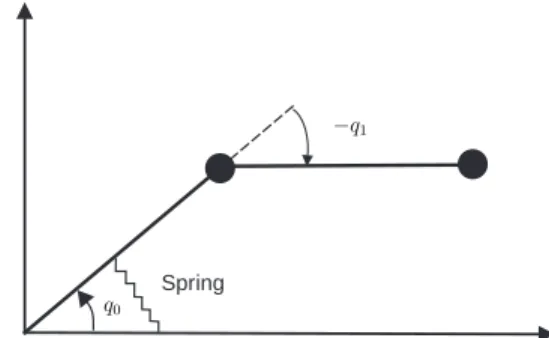
B. Planar Two-link Structure Attached to a Pivot

The purpose of the example is to emphasize the role of the potential energy in determining whether generalized momentum is conserved, and to demonstrate in the simplest possible setting the computations needed to apply Theorem 1 in order to achieve asymptotic stabilization of an equilibrium. The robot consists of two point masses connected by two rigid, massless links, with the links joined by an actuated revolute joint (the use of a distributed mass model would not change any of the following analysis). The connection to the pivot is unactuated and frictionless.

The configuration variables are chosen asq0andq1, whereF

q0 is the angle of the first link referenced to a world frame

attached to the pivot point andq1is the relative angle between

links one and two. A linear spring of stiffnessKsis introduced

between the first link and the world frame, with rest position

q0= 0. The plane of movement is assumed to be horizontal,

and thus the acceleration due to gravity is g0 = 0. The case

where the gravity is non zero can be found in [5].

1) Mathematical representation: The dynamic model is

easily obtained with the method of Lagrange and verifies that q0 is a cyclic variable. The complete dynamic model is

not given; instead, the system is immediately written in the modified normal form (11) as

˙q0 = _d0σ,0 − d0,1 d0,0˙q1 ˙σ = G0 ¨ q1 = v1 (38) where, d0,0 = a00+ a01cos(q1) d0,1 = a10+ a11cos(q1) a00 = (m1+ m2)L21+ m2L22 a01 = 2a11 a10 = m2L22 a11 = m2L1L2 G0 = −_∂q∂V0 = −Ksq0. (39)

In the above, note thatσ, given by (9), is the usual angular

momentum of the robot about the attachment point. Since the robot is constrained to a horizontal plane, if the spring constant were zero, then angular momentum would be conserved and asymptotic stabilization to an equilibrium point would be impossible.

2) Control Law Design: The control law design consists

of the preliminary feedback needed to place the system in the (modified) normal form (as explained in the Appendix), the definition of an output, and a second static state feedback used to linearize and stabilize the resulting input-output map. For the two-link robot, the output is selected as

y = K(p1− pe1) + σ, (40)

Spring

q0

−q1

Fig. 3. A two-link robot attached to a pivot and constrained to move in a horizontal plane. The joint q1is actuated, while q0is passive; a linear spring

with stiffness Ks is attached with rest position q0 = 0. From left to right,

the links have length L1 and L2and the masses are m1, m2.

where K > 0 is to be chosen, p1 = q0+a_a1101q1+ 2 µ a10 √ a2 00−a 2 01 − a00a11 a01√a200−a 2 01 ¶ · · arctan µ a00−a01 √ a2 00−a 2 01 tan(q1 2) ¶ , (41) andpe

1 is the value of p1 at the equilibrium of interest,qe.

For single-input systems, the dynamic extension (17) is trivial:v1= w1. Since it only amounts to relabelling the input,

it is dropped. Direct calculation confirms that y has relative

degree three: ˙y = K σ d0,0+ Ksq0 ¨ y = KhKs_dq00,0 − σ d2 0,0 ∂d0,0 ∂q1 ˙q1 i + Ks h σ−d0,1q˙1 d0,0 i y(3) _{= M v + N,} (42) where, M = −K σ d2 0,0 ∂d0,0 ∂q1 − Ks d0,1 d0,0 N = KhKs_dq0˙0,0− 2Ks q0 d2 0,0 ∂d0,0 ∂q1 ˙q1+ σ d3 0,0( ∂d0,0 ∂q1 ˙q1) 2 − σ d2 0,0 ∂2 d0,0 ∂2 q1 ˙q 2 1 i + Ks h Ks_dq00,0 − ∂d0,1 ∂q1 ˙ q2 1 d0,0− ( σ−d0,1q˙1 d2 0,0 ) ∂d0,0 ∂q1 ˙q1 i . (43) Suppose that M (qe_{) 6= 0. Let real scalars ¯K}

2, ¯K1 and ¯K0

be chosen such thaty(3)₊P2

j=0K¯jy(j)= 0 is exponentially

stable. Then (43) leads to the locally input-output linearizing and exponentially stabilizing control law [22]

v = 1

M (q)£−N(q, ˙q) − ¯K2y − ¯¨ K1˙y − ¯K0y¤ . (44)

The actual torque applied to the actuated joint is computed from (75) of the Appendix.

3) Simulation: For the simulations, the robot is assumed

constrained to a horizontal plane (g0= 0), the spring attaching

the first link to the reference frame is assumed linear with stiffness Ks = 5, and the model parameters are selected as

L1= 0.5, L2= 0.75, m1= 7, and m2= 7. The equilibrium

point was chosen asqe

pe

1= −0.4068, and satisfies M(qe) 6= 0. The scalars ¯Kj were

arbitrarily chosen to place the eigenvalues of the error equation at_{−1.3. The free parameter in the output was arbitrarily set to}

K = 4. Since d0,0(qe) ≈ 5, the zero dynamics has a slightly

slower speed of convergence than the output error equation. The state feedback controller (44) was simulated for the initial condition q0 = π/4, q1 = π/4, ˙q0 = 0, ˙q1 = 0.

Figure 4 shows the evolution of the commanded output and its derivatives along with the evolution of the configuration variables of the robot. The output rapidly converges to zero and the configuration variables converge to the desired equilibrium point. An animation of the motion is available at [19].

0 2 4 6 8 10 −5 0 5 10 0 2 4 6 8 10 −6 −4 −2 0 2 0 2 4 6 8 10 −5 0 5 0 2 4 6 8 10 −0.2 0 0.2 0.4 0.6 0.8 0 2 4 6 8 10 −1 −0.5 0 0.5 1 1.5 y1 ˙y1 ¨y1 q0e q1e q0 (De g ) q1 (De g) q0 q1 Time (sec) Time (sec) Time (sec) Time (sec) Time (sec)

Fig. 4. Stabilization to an equilibrium. The figure shows the convergence of the commanded output, its first two derivatives, and the configuration variables.

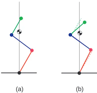
C. Planar Three-Link Serial Structure Attached to a Pivot

This example treats the planar three-link robot depicted in Figure 5. The robot consists of three point masses connected by three rigid, massless links, with the links joined by an actuated revolute joint. The connection to the pivot is unac-tuated and frictionless. The links are labelled L1 through L3

starting from the pivot and the masses are similarly labelled

m1 through m3. The parameter values given in Table I were

selected to approximate the biped robot RABBIT with the legs held together [7]. The configuration variables are chosen asq0

through q2, where q0 is the angle of the first link referenced

to a world frame attached to the pivot point, q1 is the relative

angle between links one and two, andq2 is the relative angle

between links two and three. No springs are used. The plane of movement is assumed to be vertical, and thus the acceleration due to gravity is g0= 9.81.

The example further illustrates the application of Theorem 1 through the use of an output component that has relative degree three with respect to only one of the input components and the use of a non-trivial dynamic extension in the design of the feedback controller. Both local asymptotic tracking and exponential stabilization to an equilibrium point are demon-strated.

1) Mathematical representation: The complete dynamic

model is easily obtained using the method of Lagrange and

(a)

(b)

Fig. 5. Three-link mechanism, connected at a pivot, consisting of point masses and massless bars. The links have length L1 through L3starting at

the pivot; the masses are m1through m3. (a) shows an equilibrium pose with

the center of gravity centered over the pivot; (b) shows the initial condition used in the simulation, with the equilibrium position superimposed in the background.

yields immediately the modified normal form (11) as

˙q0 = _dσ0,0− d0,1 d0,0˙q1− d0,2 d0,0˙q2 ˙σ = G0 ¨ q1 = v1 ¨ q2 = v2, (45) where, a00 = (m1+ m2+ m3)L21+ (m2+ m3)L22+ m3L23 +2m3L2L3cos(q2) a01 = 2(m2+ m3)L1L2+ 2m3L1L3cos(q2) a02 = −2m3L1L3sin(q2) a10 = (m2+ m3)L22+ m3L23+ m3L23 +2m3L2L3cos(q2) a11 = (m2+ m3)L1L2+ m3L1L3cos(q2) a12 = −m3L1L3sin(q2) d0,2 = m3L3(L2cos(q2) + L1cos(q1+ q2)) G0 = −_∂q∂V0(q) = g0(m1+ m2+ m3)L1cos(q0) +g0(m2+ m3)L2cos(q0+ q1) +g0m3L3cos(q0+ q1+ q2), (46) withd0,0,d0,1 as given in Lemma 2, (35). Note thatσ is the

angular momentum of the robot about the attachment point and is computed from the above data via (9).

2) Control Law Design: The goal is to demonstrate local

exponential stability and asymptotic tracking about an equi-librium point. An equiequi-librium point (qe_{, 0) was found from}

∂V ∂q0(q)(q

e_{) = 0, q}e

0= π/3, and q0e+ q1e+ q2e= π/3, resulting

inqe_{= (1.0472, 1.4522, −1.4522); see Figure 5 (a).}

The control law design consists of the preliminary feedback needed to place the system in the (modified) normal form (as

Link 1 Link 2 Link 3

length (m) 0.4 0.4 0.3

mass (kg) 6.4 13.6 12.0

TABLE I

MASS AND LENGTH PARAMETERS FOR THREE-LINK MECHANISM.

explained in the Appendix), the selection of two outputs, the dynamic extension that renders the system statically decou-plable (and hence statically input-output linearizable), and a second static state feedback used to linearize and stabilize the input-output map. For the three-link robot, the outputs have been selected as

y1 = Kp1+ σ

y2 = q2− q2e,

(47) where K > 0 is to be chosen, and the function p1 is

determined this time via Remark 8. The dynamic extension is

v1 = w1

˙v2 = w2,

(48) which consists of adding a single integrator on v2. Introduce

a state vector x = (q0, σ, q1, ˙q1, q2, ˙q2, v2), and express the

composition of (45), (47), and (48) as

˙x = f (x) + g(x)w

y = h(x). (49)

Direct calculation confirms thaty has (vector) relative degree

three [22] with respect to w. Indeed, using Lie derivative

notation, the output derivatives are

˙y = Lfh(x) ¨ y = L2 fh(x) y(3) _{= L}3 fh(x) + LgL2fh(x)w, (50)

whereLgL2fh corresponds to the decoupling matrix M in (21).

Evaluating the right hand side of (22) at the equilibrium point gives_{−2.35, and thus the decoupling matrix is invertible in a} neighborhood of this point. It follows that a feedback law that provides asymptotic tracking is [22]

w =£LgL2fh ¤−1  yr(3)− L3fh + 2 X j=0 ¯ Kj ³ y(j)r − L j fh ´  , (51) for any constant matrices ¯Kj that render the error equation

exponentially stable: e(3) +P2

j=0K¯je(j) = 0, for e :=

(yr− y) .

For the simulation, the matrices ¯Kj were arbitrarily chosen

to be diagonal and to place all of the eigenvalues of the error equation at _{−1. The free parameter in the output was} arbitrarily chosen as K = 5. Since d0,0(qe) ≈ 14.5, the zero

dynamics is about one third as fast as the output error equation.

3) Simulation results: The simulation demonstrates

asymp-totic tracking and exponential stabilization. The initial condi-tion was taken as _{(1.1, 1.42, −1.80, 0, 0, 0), and is depicted} in Figure 5 (b). For the first forty seconds, the robot is commanded to track sinusoidal references that cause it to

0 10 20 30 40 50 −0.4 −0.3 −0.2 −0.1 0 0.1 0 20 40 60 −2 −1.8 −1.6 −1.4 −1.2 0 20 40 60 −150 −100 −50 0 50 100 150 200 250 0 20 40 60 −150 −100 −50 0 50 100 150 y1 y2 y1 y2 y1,ref y2,ref q0 q1 q2 u1 u2 C on fig. V ar iab le s (De g) T or q u es (N) Time (sec) Time (sec)

Fig. 6. Demonstration of asymptotic tracking and stabilization for the three-link mechanism. For the first forty seconds, the motion consists of an initial transient, followed by tracking of sinusoidal trajectories that correspond to knee bends. At forty seconds, the reference trajectory is abruptly set to zero, thereby commanding the system to an equilibrium point.

execute a form of calisthenics, namely, deep knee bends; at forty seconds, the references are abruptly set to constant values corresponding to the equilibrium point qe _{in order}

to demonstrate convergence to a constant set point. The asymptotic convergence of the outputs to the commanded references is shown in Figure ??, along with the evolution of the configuration variables and the applied joint torques. An animation of the motion is available at [19].

D. Planar Two-Link Structure in Ballistic Motion

This examples illustrates how the locally linearizing coordi-nates of Theorem 2 can be used to advantage in planning a flip gait in a planar two link structure undergoing ballistic motion. The boundary constraints chosen in the flip gait are motivated by bipedal running [8]. The singularities in the decoupling matrix will be explicitly computed and related to configuration changes of the mechanism.

As shown in Figure 7, the mechanism consists of three point masses joined by two massless bars in an actuated, revolute joint. The four configuration variables are selected as q0,q1,

xc, andyc, whereq0relates the orientation of the mechanism

to a world frame and q1 is the relative angle between the

two links. The mechanism’s position with respect to a world frame is represented by the Cartesian coordinates of its center of mass. The point masses are given bym0,m1,m2; the bar

connectingm0 tom1 has length L1 and that connecting m1

tom2 has length L2.

1) Mathematical representation: The complete dynamic

model is easily obtained using the method of Lagrange and yields immediately the modified normal form (11)

˙q0 = σ−d_d0,00,1_(q(q₁1₎) ˙q1 ˙σ = 0 ¨ q1 = v ¨ xc = 0 ¨ yc = g0, (52)

q0

−q1

xc

yc

Fig. 7. A two-link robot undergoing ballistic motion in a vertical plane. Only the joint q1is actuated. From left to right, the links have length L1and

L2and the masses are m0, m1, m2.

with control v and

d0,0(q1) = a00+ a01cos(q1) d0,1(q1) = a10+ a11cos(q1) a00 = m 0(m1+m2)L 2 1+m2(m0+m1)L 2 2 m0+m1+m2 a01 = 2a11 a10 = m2(m0+m1)L 2 2 m0+m1+m2 a11 = _mm00+mm21L+m1L22. (53)

The strongly accessible portion of the model has dimension three, and involvesq0, q1, ˙q1. Due to ballistic motion, there is

a five dimensional uncontrollable subsystem that is completely decoupled from the actuated portion of the model, and this is given by xc, yc, σ, ˙xc, ˙yc. How these two parts interact in a

path planning problem is explained next.

2) Interaction through boundary conditions: The flight

phases of a gymnastic robot, such as a tumbler or a bipedal runner, are typically short-term motions that alternate with single support phases4_{. The creation of an overall satisfactory}

motion is closely tied to achieving correct boundary conditions at the interfaces of the flight and single support phases. The state of the robot at the end of a flight phase determines the ini-tial conditions for the single support phase, and consequently the state of the robot at the end of a flight phase is typically more important than the exact trajectory followed during the flight phase.

At the beginning and end of a flight phase, the robot is in contact with a surface, assumed here to be identified with the horizontal component of the world frame. Assume furthermore that the robot is in single support, with the contact point being either the mass m0 or m2. In single support, there are

two holonomic constraints that tie the position and velocity of the center of mass to those of the angular coordinates; in other words, there is a loss of two degrees of freedom. Conservation of angular momentum through ˙σ = 0 yields an

additional (nonholonomic) constraint on the angular velocities. In particular, the desired final joint velocities must be chosen to satisfy this constraint.

4_{That is, one end of the mechanism is in contact with a rigid surface, and}

the contact point is neither slipping nor rebounding; in other words the contact point is acting as a pivot.

The duration of the flight phase,T, is determined from ¨yc=

g0, with the initial conditions coming from the initial positions

and velocities of the angular coordinates at lift-off, and the end condition of the height of the center mass coming from the desired final configuration of the angular coordinates at touch-down. Once the flight time is known, determining whether or not there exists a solution of the reduced model,

˙q0 = σ−d_d0,00,1_(q(q₁1₎) ˙q1

¨

q1 = v,

(54) that is compatible with a given set of initial and final con-ditions is a difficult problem: once a trajectory for q1(t) is

chosen, ˙q0 must be numerically integrated, and ifq0(T ) does

not have the desired value, thenq1(t) must be altered. Such an

iterative procedure is poorly adapted to on-line computations. Theorem 2 will be applied to simplify this task. It should be noted that the value of the momentum σ is unknown before

the start of the flight phase, and thus it is not even possible to determine the reduced model (54) before the initial condition of the robot is known at lift-off.

3) Determining a ballistic motion trajectory in linearizing coordinates: Local, input-output linearizing coordinates for

the reduced model (54) are constructed from y = p1 and its

first two derivatives. Define p1 by (41). Direct computation

leads to ˙p1 = σ d0,0(q1) = σ a00+ a01cos(q1) (55) ¨ p1 = σ d dq1d0,0(q1) d0,0(q1)2 ˙q1= σa01sin(q1) (a00+ a01cos(q1))2 ˙q1. (56)

To determine the linearizing control, one more derivative is needed

p(3)₁ = σa01

(2a01+ a00cos(q1) − a01cos2(q1))

(a00+ a01cos(q1))3 ˙q2 1 + M1,1v (57) M1,1 = σ d dq1d0,0(q1) d0,0(q1)2 = σa01sin(q1) (a00+ a01cos(q1))2 . (58) WhereverM1,16= 0, a linearizing feedback can be constructed

such that

p(3)1 = w. (59)

For arbitrary initial and final conditions of the linear model (59), it is trivial to define a feasible trajectory. Indeed, it suffices to define a three-times continuously differentiable function passing from given initial values to given final values. One could even use a polynomial of order five or greater.

Since the change of coordinates going from (54) to (59) is local, not every solution of (59) can be mapped back onto a solution of (54). From (55),p1, the “global” orientation of the

robot, can only be changed through modification of the inertia parameter, d0,0, because the angular momentum is constant.

The inertia termd0,0can only be changed through variation of

the internal angle,q1. Since d0,0 is bounded, so is ˙p1. These

kinds of constraints, which must be applied point-wise in time on the trajectories of (59), are made explicit by computing the inverse of the coordinate change.

4) Constraints point-wise in time associated with the lin-earizing coordinates: The calculation ofq0, q1, ˙q1in terms of

p1, ˙p1, ¨p1 yields q1 = arccos( σ ˙ p1 − a00 a01 ) (60) q0 = p1− a11 a01 q1− 2 à a10 pa2 00− a201 − a00a11 a01pa200− a201 ! · · arctan à a00− a11 pa2 00− a201 tan(q1 2 ) ! (61) ˙q1 = ¨ p1(a00+ a01cos(q1))2 σa01sin(q1) (62) The first equation only admits a solution for _a σ

00−a01 ≤ ˙p1≤

σ

a00+a01, and then has two solutions: one for 0 ≤ q1 < π

and another for _{−π ≤ q}1 < 0. These two domains for the

cosine define two “configuration classes” of the robot, with the extreme points of the domains corresponding to the links being completely folded or unfolded. At the extreme points of the domains, ˙p1 attains an extremum and consequently, p¨1

is zero. At an extreme point of q1, ˙q1 cannot be determined

from (62), which takes the form ˙q1=0₀. SinceM1,1 vanishes

at an extreme point, (57) is used withM1,1= 0 to obtain

˙q1= ±

s p(3)1

(a00+ a01cos(q1))3

σa01(2a01− a01cos2(q1) + a00cos(q1))

,

(63) with the sign of ˙q1 being determined by continuity (with

torque control, there cannot be discontinuities in the velocity). The robot will then pass through the singularity, and change configuration classes.

Consequently, when generating a motion, two cases can present themselves, according to whether the motion stays always in the same configuration class or not. If the initial and final configuration are in the same configuration class, then a trajectory can be generated by imposing _a σ

00−a01 <

˙p1(t) < _a00+aσ 01. Both open-loop and feedback controls are

equally easily computed starting from the linear model. If the initial and final configurations are in different configuration classes, a trajectory can be computed that passes through a singularity at a single time instance,_{0 ≤ t}0≤ T, where M1,1

vanishes. An open-loop control can be determined as before. On the other hand, a feedback implementation is not possible based on inverting M1,1 in (58). However, since the flight

phase is typically of short duration and the input is calculated as a function of the initial conditions, an open-loop control is probably sufficient.

5) Simulation without passing through a singularity: The

model parameters were selected asL1= 1.0, L2= 1.0, m0=

1.0, m1 = 2.0, m2 = 1.0 For this simulation, the mass m0

of the robot is supposed initially in contact with the ground, with configuration defined by q0 = 3π/4, q1 = −π/4, and

angular velocities ˙q0= −5, ˙q1= 0. The objective is to transfer

the robot at the end of a flight phase so that when the mass

m2of the robot touches the ground, its configuration is q0=

−0.5, q1 = −π/4 with angular velocity proportional to ˙q0=

1, ˙q1 = 0. The initial and final configurations are depicted

in Figure (8); they belong to the same configuration class. From the initial conditions of the robot and the desired final configuration, the flight time is computed as T = 0.5173.

Conservation of angular momentum implies that ˙q0(T ) = −5.

1 0.5 0 0.5 1 1.5 2 0 0.5 1 1.5 2

Fig. 8. The motion of the robot passes from left to right without passing through a singularity. The initial configuration (· − ·− green) and final configuration (· − ·− red) belong to the same configuration class. The center of gravity follows a parabolic trajectory.

The initial and final values ofp1and its first two derivatives

were computed from (41), (55), and (56). A fifth-order polyno-mial oft was defined that satisfied these boundary conditions.

The resulting trajectories of p1, ˙p1, ¨p1 are depicted in Figure

9; the point-wise in time constraints associated with (60), (61) and (62) are met. The input torque u for the system was

computed using (57) and (75) of the Appendix. The resulting trajectories in terms of q and ˙q are shown in Figure 10 and

the evolution of the robot in the vertical plane is presented in Figure 8. An animation of the motion is available at [19].

0 0.05 0.1 0.15 0.2 0.25 0.3 0.35 0.4 0.45 0.5 −1 0 1 2 0 0.05 0.1 0.15 0.2 0.25 0.3 0.35 0.4 0.45 0.5 −9 −8 −7 −6 −5 0 0.05 0.1 0.15 0.2 0.25 0.3 0.35 0.4 0.45 0.5 −5 0 5 p1 ˙p1 ¨p1 Time (sec)

Fig. 9. Based on the initial and final conditions of the flight phase, a trajectory for p1and its derivatives is derived. The plot shows thatp satisfies˙

the constraint σ

a00−a01 ≤ ˙p1(t) ≤

σ a00+a01

6) Simulation with passage through a singularity: For this

simulation, the mass m0 of the robot is supposed initially

in contact with the ground, with configuration defined by

q0= 3π/4, q1= π/4 and angular velocities ˙q0= −5, ˙q1= 0.

0 0.1 0.2 0.3 0.4 0.5 −1 0 1 2 3 0 0.1 0.2 0.3 0.4 0.5 −2 −1.5 −1 −0.5 0 0 0.1 0.2 0.3 0.4 0.5 −8 −7 −6 −5 −4 −3 0 0.1 0.2 0.3 0.4 0.5 −5 0 5 q0 q1 ˙q0 _˙q1 Time (sec) Time (sec) Time (sec) Time (sec)

Fig. 10. The computed open-loop control transfers the robot from its initial state to the desired final state (*).

phase so that when the mass m2 of the robot touches the

ground, its configuration is q0 = −0.5, q1 = −π/4 with

angular velocity proportional to ˙q0 = 0, ˙q1 = 1. The initial

and final configurations are depicted in Figure (11); they do not belong to the same configuration class. From the initial conditions of the robot and the desired final configuration, the flight time is computed as T = 0.7062s. Conservation of

angular momentum implies that ˙q0(T ) = −5.

1.5 1 0.5 0 0.5 1 1.5 2 0 0.5 1 1.5 2

Fig. 11. The motion of the robot passes from left to right, with a singular position occurring when the two links are aligned. The initial configuration (·− ·− green) and final configuration (·−·− red) belong to different configuration classes.

The initial and final values ofp1and its first two derivatives

were computed as before. So that the robot changes config-uration class, at ts = T /2, the trajectory was forced to pass

through a singularity corresponding to q1= 0, that is, ¨p1= 0

and ˙p1 = σ/(a00 + a01). A seventh-order polynomial in t

was defined that satisfied the six boundary conditions, plus

¨

p1(ts) = 0, ˙p1(ts) = σ/(a00+ a01). The resulting trajectories

of p1, ˙p1, ¨p1 are depicted in Figure 12. The corresponding

trajectories in terms of q and ˙q are shown in Figure 13 and

the evolution of the robot in the plane is presented in Figure 11. An animation of the motion is available at [19].

0 0.1 0.2 0.3 0.4 0.5 0.6 0.7 −1 0 1 2 0 0.1 0.2 0.3 0.4 0.5 0.6 0.7 −9 −8 −7 −6 −5 0 0.1 0.2 0.3 0.4 0.5 0.6 0.7 −5 0 5 p1 ˙p1 ¨p1 Time (sec)

Fig. 12. Based on the initial and final conditions of the flight phase, a trajectory for p1 and its derivatives is derived. The plot shows thatp˙1 hits

the constraint σ

a00+a01 in the middle of the flight phase, which allows the change in the configuration class to occur.

0 0.2 0.4 0.6 0.8 −1 −0.5 0 0.5 1 1.5 2 2.5 0 0.2 0.4 0.6 0.8 −1.5 −1 −0.5 0 0.5 1 1.5 0 0.2 0.4 0.6 0.8 −8 −6 −4 −2 0 0 0.2 0.4 0.6 0.8 −10 −5 0 5 10 Time (sec) Time (sec) Time (sec) Time (sec) q0 q1 ˙q0 _˙q1

Fig. 13. The computed open-loop control transfers the robot from its initial state to the desired final state (*).

V. ADDITIONALTECHNICALPOINTS

This section provides additional discussion on a few points that would have broken the flow of the main developments.

A. A cascade structure

The feedback designs of Section III-C that have been illustrated on the two-link and three-link models have sin-gularities where the decoupling matrix looses rank. Results in [20] show that (within the category of analytic systems and compensators) achieving an invertible decoupling matrix via dynamic compensation is a necessary condition for the existence of a compensator that achieves asymptotic tracking of an open set of reference trajectories. Hence, while it is not necessary that the particular decoupling matrix constructed in (21) be invertible, at least some other decoupling matrix would have to be invertible for asymptotic tracking to be possible on a larger set.

If one is only trying to accomplish stabilization on a large set and not asymptotic tracking, it is then interesting to consider feedback designs that avoid the requirement of an invertible decoupling matrix. One way that this may be

approached for the systems studied in Section III-C is the following. First, use (13) to rewrite (11) in the coordinates (p1, σ, q1, · · · , qN −1, ˙q1. . . ˙qN −1) as ˙p1 = _d0,0(q1,··· ,qσ _{N −1})+ PN −1 k=2 Jk(q1, · · · , qN −1) ˙qk ˙σ = G¯0(p1, q1, · · · , qN −1) ¨ qj = vj, j = 1, · · · , N − 1, (64) where ¯ G0(p1, q1, · · · , qN −1) := −∂V ∂q0(q0, q1, · · · , qN −1) ¯ ¯ ¯ q0=p1+qe0− Rq1 qe1 d0,1 d0,0(τ,q2,··· ,q_{N −1})dτ . (65) Define x1 = (p1, σ)′, x2 = q1, x3 = ˙q1, x4 = (q2, · · · , qN −1)′, x5 = ( ˙q2, · · · , ˙qN −1)′, v¯1 = v1 and ¯v2 =

(v2, · · · , vN −1)′. Then (64) takes the form of a feedforward

nonlinear system ˙x1 = f1(x1, x2, x4) + g1(x2, x4)x5 ˙x2 = x3 ˙x3 = ¯v1 ˙x4 = x5 ˙x5 = ¯v2, (66)

for which various feedback stabilization methods have been developed [30, 48, 49, 55]. Backstepping suggests considering

x2 and x5 as virtual controls [28], leading to the simpler

(block-)feedforward system

˙x1 = f1(x1, x2, x4) + g1(x2, x4)x5

˙x4 = x5. (67)

For a two-link system,x4andx5are empty, leading to the two

dimensional system ˙x1 = f1(x1, x2), the global asymptotic

stabilization5 of which has been studied in [36]. The problem of asymptotically stabilizing (67) on large sets is open for systems with three or more links.

B. Checking feedback linearizability

This subsection offers a few observations on the generic non-feedback linearizability of the model class studied here when generalized conjugate momentum is not conserved. The reason to check this property is that if the systems were feedback linearizable, then it would be possible to achieve an empty zero dynamics instead of a zero dynamics with dimension one. Recall that for single-input systems, it is known that a system is dynamically feedback linearizable if, and only if, it is statically feedback linearizable. For multi-input systems, dynamic feedback does enlarge the class of linearizable systems, but necessary and sufficient conditions for dynamic feedback linearizability are not known. If one restricts the outputs used to achieve dynamic feedback lineariz-ability (often called flat outputs) to being only functions of the configuration variables, however, then for mechanical systems with one degree of underactuation, necessary and sufficient 5_{The Lyapunov function used in [36] was not shown to be proper or radially}

unbounded. For the Acrobot, a periodicity property of ¯G0can be used to fill

this lacuna when the dynamic model is extended in the obvious way to IR4_.

conditions for dynamic feedback linearization are known [43]; in particular, for the class of systems being studied in this paper, the conclusion is that there do not generally exist flat outputs depending only on the configuration variables.

Consider first a 2-DOF system written in the form of (64), and suppose that ¯G0 6= 0. Such a system has a single input

and thus necessary and sufficient conditions for feedback linearizability can be checked. Applying the method of [11], the system is feedback linearizable if, and only if,

• either _dqd

1(d0,0) ≡ 0, in which case p1is a linearizing (or

flat) output, • or, _dqd 1(d0,0) 6≡ 0 and d dq1(β) ≡ 0, where β = µ d2 0,0 d dq1(d0,0) ∂ ¯G0 ∂q1 ¶ , in which case σ2_+2βp 1is a linearizing

(or flat) output.

These conditions are not generally satisfied for the class of systems being studied; in particular, applying them to the two link example of Section IV-B proves that it is not feedback linearizable.

Consider next a system with 3-DOF written either in the form (11) or (64). Applying once again the method in [11], the system is statically feedback linearizable only if

∂J2

∂q1 ≡ 0;

(68) moreover, the same obstruction persists if an integrator is added on v2 so the dynamic extension used in the paper

does not render the system static feedback linearizable. The obstruction (68) is present in the three link example of Section IV-C.

We know of only two mechanical systems that meet the conditions of this paper and are feedback linearizable: the inertia wheel pendulum [54] and the RTAC or TORA (see [23] and references therein). Both systems satisfy the condition

d

dq1(d0,0) ≡ 0, and thus p1is a linearizing output. The method

of this paper also finds the locally linearizing coordinates. This is shown only for the inertia wheel pendulum.

In the coordinates of Figure 1, the modified normal form of the inertia wheel pendulum is

˙q0 = _dσ_0,0−d_d0_0,0,1˙q1 ˙σ = G0 ¨ q1 = v1, (69) where d0,0 = m1l2c1+ m2l12+ I1+ I2 d0,1 = I1 G0 = mg¯ 0cos(q0) ¯ m = m1lc1+ m2l1, (70)

and the parameters are as defined in [54]. Sinced0,0 andd0,1

are constant, (6) is trivially integrated about the equilibrium pointqe_{= (π/2, 0, 0, 0) to obtain}

p1= (q0− π/2) +

d0,1

d0,0q1.

(71) Defining the output as y = Kp1+ σ and using (13) and