Blooms of the toxic dinoflagellate Alexandrium fundyense in the Gulf of Maine : investigations using physical-biological model

Blooms of the Toxic Dinoflagellate Alexandrium fundyense in the

Gulf of Maine: Investigations Using a Physical-Biolo

By Charles A. Stock

B.S.E., Princeton University, 1997 M.S., Stanford University, 1998

ical Model

Submitted in partial fulfillment of the requirements for the degree of DOCTOR OF PHILOSOPHY

at the

MASSACHUSETTS INSTITUTE OF TECHNOLOGY and the

WOODS HOLE OCEANOGRAPHIC INSTITUTION February 2005

C 2005, Charles A. Stock All rights Reserved

The author hereby grants to MIT and WHOI permission to reproduce paper and electronic copies of this thesis in whole or in part and to distribute them publicly.

Signature of Author

Joint Program in Oceanography/Applied Ocean Science and Engineering Massachusetts Institute of Technology and Woods Hole Oceanographic Institution February, 2005 Certified by / / Dennis J. McGillicuddy Thesis Supervisor Accepted by

-7

Blooms of the Toxic Dinoflagellate Alexandrium fundyense in the Gulf of

Maine: Investigations using a Physical-Biological Model

by

Charles A. Stock

MIT/WHOI Joint Program in Oceanography and Oceanographic Engineering Submitted to the Massachusetts Institute of Technology/Woods Hole Oceanographic Institution Joint Program in Oceanography and Oceanographic Engineering on December 21, 2004 in partial fulfillment of

the requirements for the Degree of Doctor of Philosophy

ABSTRACT

Blooms of the toxic dinoflagellate Alexandriumfundyense are annually recurrent in the western Gulf of Maine (WGOM) and pose a serious economic and public health threat. Transitions between and vital rates within the life stages of A. fundyense are influenced by diverse environmental factors, and these biological dynamics combine with energetic physical motions to yield complex bloom patterns. In this thesis, a biological model of the A. fundyense life cycle developed from laboratory and field data is combined with a

circulation model to test hypotheses concerning the factors governing A. fundyense blooms in the springs of 1993 and 1994.

There is considerable uncertainty with the biological dynamics, and several biological model structures are tested against the 1993 observations. Maximum likelihood theory is used to evaluate the statistical significance of changes in model/data fit between

structures. Biological formulations that do not include either nitrogen limitation or mortality overestimate observed cell abundances and are rejected. However,

formulations using a wide range of mortality and nitrogen dependence, including the exclusion of one or the other, were able to match observed bloom timing and magnitude and could not be statistically differentiated. These simulations suggest that cysts

germinating offshore of Casco Bay provide a plausible source of cells for the blooms, although cell inputs from the eastern Gulf of Maine gain importance late in the spring and in the northeast portion of the study area. Low net growth rates exert a notable yet non-dominant influence on the modeled bloom magnitude.

When simulations tuned to 1993 were applied to 1994 the degree of model/data fit is maintained only for those simulations including nitrogen dependence. The model suggests that differences in toxicity between the two years result from variability in the wind and its influence on the along and cross-shore transport of cells. Extended simulations generally predict a proliferation of A. fundyense abundance in mid-June within areas of retentive circulation such as Cape Cod Bay. This proliferation is not observed, and better resolution of the losses and limitations acting on A. fundyense is needed at this stage of the bloom.

Thesis Supervisor: Dennis J. McGillicuddy

4

-Acknowledgements

This work would not have been possible were it not for the efforts of many. I would like to start by thanking my advisor, Dennis McGillicuddy for his guidance, patience, and clarity of thought. I would also like to thank my committee members: Don Anderson, Dan Lynch, and Penny Chisholm for all of their advice and efforts on my behalf. The time and insight of the investigators on the ECOHAB-Gulf of Maine and RMRP programs is also greatly appreciated. Particular gratitude in this regard is due to Andy Solow, Bruce Keafer, John Cullen, Rich Signell, Ted Loder, Paty Matrai and Dave Townsend. Penny and Ole Madsen contributed greatly to the success and enjoyment of my studies while at MIT, and I thank them for this. I would also like to that Peter Franks for his encouragement. The diverse interests of the scientists of the Department of Applied Ocean Physics and Engineering, especially those within the Coastal Ocean and Fluid Dynamics Laboratory were a constant source of inspiration, and I thank them for their generosity and open doors. I would like to particularly recognize Ruoying He for his modeling insights during the final year of my studies. I would also like to thank Olga Kosnyreva, my officemate during my time at Woods Hole, for her warmth, kindness, and tolerance of my filing system (or lack thereof). Gratitude is also due to the Woods Hole Academic Programs Office for their support, guidance, and never-ending patience. Finally, I would like to end by earnestly thanking my family and friends for all of their support, warmth, generosity, and humor over the past years. Particular gratitude is due to my parents, my brother, and Nancy - thank you.

This research was funded by EPA STAR fellowship 91574901, National Science Foundation Grant OCE-9808173, and the WHOI Academic Programs Office. This generous support is gratefully acknowledged.

Table of Contents:

1. Introduction 9

2. The Application of Maximum Likelihood Estimation Theory to a Physical-Biological Modeling Study of Harmful Algal Blooms in the Gulf of Maine 19

3. Evaluating hypotheses for the initiation and development of Alexandrium

fundyense blooms in the western Gulf of Maine using a coupled physical-biological

model 85

4. A Comparative Modeling Study of Blooms of the Toxic Dinoflagellate

Alexandrium fundyense in the western Gulf of Maine in 1993 and 1994

5. Summary

6. Appendix A: The Germination Model

143

211

223

259 7. Appendix B: The Growth Model

8

Chapter 1

Blooms of the toxic dinoflagellate Alexandriumfundyense are annually recurrent phenomena in the Gulf of Maine during the spring and summer months. Toxins

produced by A. fundyense lead to paralytic shellfish poisoning (PSP), a potentially fatal illness caused by consumption of shellfish from exposed regions. This public health risk necessitates rigorous monitoring of potentially affected areas and has lead to repeated closures of shellfish beds along the coast and in the offshore waters of the Gulf of Maine (Shumway, et al., 1988). Within the marine food web, PSP has been linked to mortality of larval and juvenile stages of fish (White, et al., 1989), and even the death of marine mammals such as humpback whales (Geraci, et al., 1989). An understanding of the factors that determine the distribution and abundance of A. fundyense within the Gulf of Maine is therefore of considerable scientific, economic, and public health interest.

Alexandrium species are characterized by a life cycle that includes both a resting

benthic cyst and a vegetative cell (Anderson, 1998). Transitions between these stages have long been thought critical to understanding bloom dynamics in coastal waters (Anderson and Wall, 1978, Anderson, et al., 1983). The transition between resting and vegetative stages occurs through the process of germination. Rates of germination are controlled by diverse factors including light, temperature, oxygen in the sediments, and

an internal endogenous clock (Anderson, 1980, Anderson and Keafer, 1987, Anderson, et al., 1987, Anderson, et al., submitted, Matrai, et al., submitted). Upon germination, vegetative A. fundyense cells swim upward to the euphotic zone, where they undergo a stage of vegetative growth. Some strains enlist coordinated vertical migrations in response to nutrients and light during this stage (MacIntyre, et al., 1997, Cullen, et al., 2004). The vegetative growth stage terminates with the formation of gametes that fuse to

form a new cyst. The onset of encystment has been difficult to observe in the field, but it is thought to be a reaction to environmental stress and has been induced by nutrient depletion in the laboratory (Anderson, et al., 1984, Anderson and Lindquist, 1985). Blooms of A. fundyense in the Gulf of Maine do not develop in static water columns, but within a dynamical physical context characterized by energetic motions covering a broad range of scales. At the largest scales, a persistent Gulf-wide circulation is driven by density gradients between high salinity slope water in the Gulfs deep basins and fresher coastal waters derived from the Scotian shelf and local river inputs (Bigelow, 1927, Brooks, 1985, Fig. 1). This current is subdivided into a series of segments and branch points (Lynch, et al., 1997). The direction of flow at the branch points is

modulated by a diverse set of factors including wind, river input, bathymetric effects, and the strength of the geopotential low that generally forms over Jordan Basin in response to dense slope water in its interior (Brooks and Townsend, 1989, Brooks, 1994, Lynch, et al., 1997, Pettigrew, et al., 1998). Within each branch, interactions between local river inputs, bathymetry and wind forcing can create energetic motions over daily time scales and tens of kilometers (e.g. Fong, et al., 1997, Geyer, et al., 2004). A. fundyense blooms have been demonstrated to strongly interact with the physical dynamics over the full range of scales described above (Franks and Anderson, 1992a, Townsend, et al., 2001, McGillicuddy, et al., 2003, Anderson, et al., 2004a, McGillicuddy, et al., submitted-b). This interweaving of the complex life history of A. fundyense and the dynamic physical environment of the WGOM suggests the use of a coupled physical-biological model to diagnose bloom dynamics.

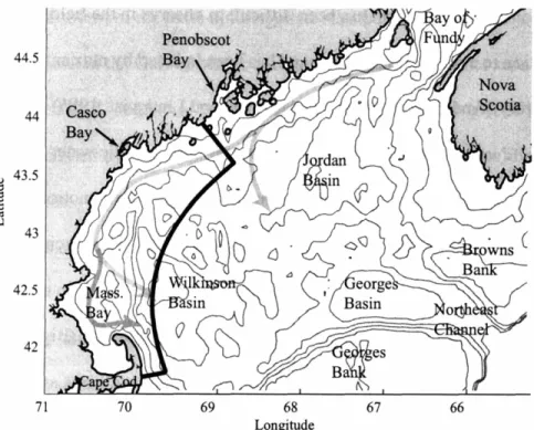
44.5 44 (l) 43.5 "'0 .€ ~ ....l 43 42.5 42 71 70 66

Figure 1: The Gulf of Maine and study region. The study domain is outlined in black. Depth contours are at 50, 100, 150 and 200 meters. The direction of flow of the Maine Coastal Current (adapted from Lynch et aI., 1997) is shown as a thick gray line. Branch points offshore of Penobscot Bay and Cape Ann are notable. The region of interest for the studies herein is the western Gulf of Maine (WGOM), and is outlined by the thick, dark line.

This thesis focuses on bloom patterns in the western Gulf of Maine, which is the region south and west of Penobscot Bay in Fig. 1. Shellfish toxicity has been observed continuously in the region since a large events toxicity events in 1972 and 1974

(Shumway, et aI., 1988). While there was initial conjecture that blooms in the region were linked to coastal upwelling (Mulligan, 1973, Hartwell, 1975, Mulligan, 1975), a series of papers by Franks and Anderson (1992a, 1992b) demonstrated that patterns of WGOM shellfish toxicity were more consistent with the along-shore advection of cells in association with the buoyant plume of the Kennebec and Androscoggin rivers. This finding led to the formulation of the "plume advection hypothesis", which consisted of several components paraphrased below:

· A source of Alexandriumfundyense in the north of the region possibly associated with the Kennebec/Androscoggin estuaries.

* A pulse of freshwater in May carries cells out of the estuaries, entrains nearshore populations, and is critical to the along-coast propagation of cells and associated shellfish toxicity.

* Upwelling winds force the river plume and cells offshore and away from shellfish beds, and downwelling winds hold the plume to the coast and increase southward transport.

This conceptual model was found to be consistent with a observations along a series of transects near Cape Ann (Franks and Anderson, 1992a), and with long terms toxicity records (Franks and Anderson, 1992b).

A second study was undertaken in 1993 and 1994 in an effort to test the dynamics of the plume advection hypothesis, and to refine and resolve its elements (Anderson, et al., 2004a, Geyer, et al., 2004). This study included broad survey coverage, as well as mooring and drifter deployments. Shellfish toxicity was prevalent along the entire coast in 1993, but was less severe in 1994 and restricted to areas north of Cape Ann.

Differences in toxicity were primarily attributed to variations in the wind forcing between the two years, with winds being more upwelling favorable in the spring of 1994

(Anderson, et al., 2004a). Potential mechanisms for the delivery of cells to inshore regions related to circulation induced around the edges of river plumes were also discussed. Finally, a "two source" model for A. fundyense cells was proposed, with one source in inshore waters near Casco Bay, and a second derived from germination within offshore cyst beds and inflows of vegetative cells from the EGOM.

In this thesis, a coupled physical-biological model is constructed to synthesize present knowledge of the physical and biological dynamics that govern A. fundyense blooms in the western Gulf of Maine. This model is compared with observations to test hypotheses concerning bloom dynamics. The primary goals are to rigorously test the plausibility of the plume advection hypothesis, to further resolve the factors controlling bloom transport and net growth, to provide quantitative estimates of various sources and sinks of cells, and to identify major remaining uncertainties.

Chapter 2 provides a detailed description of the application of maximum likelihood theory to test hypotheses concerning the parameters governing bloom

dynamics. While determined laboratory and field efforts have constrained key aspects of the biological dynamics, the potential complexity of the modeled processes and the measurement challenges inevitably produce uncertain model parameters. This problem is ubiquitous within coupled physical-biological modeling, and parameter values are often tuned within their uncertainty to best match observations. However, observations can be sparse and noisy, and approaching this procedure in a statistically rigorous fashion is essential if false conclusions regarding the parameter values are to be avoided. Chapter 2 begins by demonstrating key properties of maximum likelihood estimates and the use of the maximum likelihood ratio test to constrain parameter values using the example of a linear regression. This is followed by a detailed methodological discussion of the application of these tools for testing hypotheses concerning A. fundyense blooms in the Gulf of Maine. Particular attention is paid to pragmatic steps that must be taken in translating theory into practice. Limitations of and potential improvements to the approach are also discussed.

Chapter 3 tests the ability of four potential biological model structures to match the timing and magnitude of the observed A. fundyense bloom in the spring of 1993. The methodology applied is that described in detail within Chapter 2. The model structures are nested, in that each adds an additional degree of freedom to the prior structure. As each new parameter is added, maximum likelihood estimation is used to determine if the skill added supports the rejection of the previous model structure for the more complex alternative. The focus of the model diagnosis is the estimation of the contributions of the various sources of A. fundyense to the western Gulf of Maine, identification of the factors controlling net growth, and assessment of the impact of net growth on bloom magnitude and the cell distribution.

Chapter 4 tests a range of parameter values found optimal in 1993 against the 1994 data set to evaluate the inter-annual robustness of the model. Diagnosis focuses on the underlying physical and biological causes for the differences in A. fundyense

abundance, distribution, and associated shellfish toxicity between the two years. Central to the analysis is a series of exchanges in model forcing for the two years. Estimates of the sources and sinks of cells are provided both in a domain-averaged sense, and within specific regions (Casco Bay and within Massachusetts and Cape Cod Bays) in order to further resolve elements of the bloom dynamics.

The thesis concludes by summarizing contributions of this thesis to the understanding of A. fundyense bloom dynamics in the western Gulf of Maine. Key aspects of the hypothesis testing procedure and potential improvements are also discussed. Lastly, prospects for future model improvement are addressed.

Anderson, D. M., 1980. Effects of temperature conditioning on development and germination of Gonyaulax tamarensis (Dinophyceae) hypnozygotes. Journal of Phycology 16, 166-172.

Anderson, D. M., 1998. Physiology and bloom dynamics of toxic Alexandrium species, with emphasis on life cycle transitions. In: Anderson, D. M., Cembella, A. D. ,Hallegraeff, G. M. (Eds.), Physiological Ecology of Harmful Algal Blooms. Springer-Verlag, Berlin, pp. 29-48.

Anderson, D. M., Chisholm, S. W., Watras, C. J., 1983. The importance of life cycle events in the population dynamics of Gonyaulax tamarensis. Marine Biology 76,

179-190.

Anderson, D. M., Keafer, B. A., 1987. The endogenous annual clock in the toxic dinoflagellate Alexandrium tamarensis. Nature 325, 616-617.

Anderson, D. M., Keafer, B. A., Geyer, W. R., Signell, R. P., Loder, T. C., 2004. Toxic

Alexandrium blooms in the Gulf of Maine: the "plume advection hypothesis"

revisited. Limnology and Oceanography (submitted).

Anderson, D. M., Kulis, D. M., Binder, B. J., 1984. Sexuality and cyst formation in the dinoflagellate Alexandrium tamarensis: Cyst yield in batch cultures. Journal of Phycology 20, 418-425.

Anderson, D. M., Lindquist, N. L., 1985. Time-course measurements of phosphorous depletion and cyst formation in the dinoflagellate Gonyaulax tamarensis Lebour. Journal of Experimental Marine Biology and Ecology 86, 1-13.

Anderson, D. M., Stock, C. A., Keafer, B. A., Bronzino, A. C., Matrai, P., Thompson, B., Keller, M., McGillicuddy, D. J., Hyatt, J., submitted. Experimental and modeling observations of Alexandriumfundyense cyst dynamics in the Gulf of Maine. Deep-Sea Research, Part II

Anderson, D. M., Taylor, C. D., Armbrust, V. E., 1987. The effects of darkness and anaerobiosis on dinoflagellate cyst germination. Limnology and Oceanography 32, 340-351.

Anderson, D. M., Wall, D., 1978. Potential importance of benthic cysts of Gonyaulax

tamarensis and G. excavata in initiating toxic dinoflagellate blooms. Journal of

Phycology 14, 224-234.

Bigelow, H. B., 1927. Physical oceanography of the Gulf of Maine. Fisheries Bulletin 40, 511-1027.

Brooks, D. A., 1985. Vernal circulation in the Gulf of Maine. Journal of Geophysical Research 90, 4687-4705.

Brooks, D. A., 1994. A model study of the buoyancy-driven circulation in the Gulf of Maine. Journal of Physical Oceanography 24, 2387-2412.

Brooks, D. A., Townsend, D. W., 1989. Variability of the coastal current and nutrient pathways in the eastern Gulf of Maine. Journal of Marine Research 47, 303-321. Cullen, J. J., Wood, Barnett, Normandeau, Ryan, 2004. Behavioral and physiological

variability among strains of the toxic dinoflagellate Alexandrium fundyense from the Gulf of Maine. Deep-Sea Research, Part II (submitted).

Fong, D. A., Geyer, W. R., Signell, R. P., 1997. The wind-forced response of a buoyant coastal current: Observations of the western Gulf of Maine plume. Journal of Marine Systems 12, 69-81.

Franks, P. J. S., Anderson, D. M., 1992a. Alongshore transport of a toxic phytoplankton bloom in a buoyancy current: Alexandrium tamarense in the Gulf of Maine. Marine Biology 112, 153-164.

Franks, P. J. S., Anderson, D. M., 1992b. Toxic phytoplankton blooms in the Gulf of Maine: testing hypotheses of physical control using historical data. Marine Biology 112, 165-174.

Geraci, J. R., Anderson, D. M., Timperi, R. J., Staubin, D. J., Early, G. J., Prescott, J. H., Mayo, C. A., 1989. Humpback Whales (Megaptera novaeangliae) fatally

poisoned by dinoflagellate toxin. Canadian Journal of Fisheries and Aquatic Science 46, 1895-1898.

Geyer, W. R., Signell, R. P., Fong, D. A., Wang, J., Anderson, D. M., Keafer, B. A., 2004. The freshwater transport and dynamics of the western Maine Coastal Current. Continental Shelf Research 24, 1339-1357.

Hartwell, A. D., 1975. Hydrographic factors affecting the distribution and movement of toxic dinoflagellates in the western Gulf of Maine. In: LoCicero, V. R., (Ed.), Proceedings of the first international conference on toxic dinoflagellate blooms, Boston. Massachusetts Science and Technology Foundation, pp. 47-68.

Lynch, D. R., Holboke, M. J., Naimie, C. E., 1997. The Maine coastal current: spring climatological circulation. Continental Shelf Research 17, 605-634.

Matrai, P., Thompson, B., Keller, M. D., submitted. Alexandrium spp. from eastern Gulf of Maine: Circannual excystment of resting cysts. Deep Sea Research II

McGillicuddy, D. J., Anderson, D. M., Lynch, D. R., Townsend, D. W., 2004. Mechanisms regulating the large-scale seasonal development of Alexandrium

fundyense blooms in the Gulf of Maine. Deep-Sea Research, Part II

McGillicuddy, D. J., Signell, R. P., Stock, C. A., Keafer, B. A., Keller, M. D., Hetland, R. D., Anderson, D. M., 2003. A mechanism for offshore initiation of harmful algal blooms in the coastal Gulf of Maine. Journal of Plankton Research 25, 1131-1139.

Mulligan, H. F., 1973. Probable causes of the 1972 red tide in the Cape Ann region of the Gulf of Maine. Canadian Journal of Fisheries and Aquatic Science 30, 1363-1366. Mulligan, H. F., 1975. Oceanographic factors associated with New England red tide

blooms. In: LoCicero, V. R., (Ed.), Proceedings of the first international

conference on toxic dinoflagellate blooms, Boston, MA. Massachusetts Science and Technology Foundation, pp. 23-40.

Pettigrew, N., Townsend, D., Xue, H., Wallinga, J., Brickley, P., Hetland, R., 1998. Observations of the eastern Maine Coastal Current and its offshore extensions in 1994. Journal of Geophysical Research Vol. 103, 30,623-30,639.

Shumway, S. E., Sherman-Caswell, S., Hurst, J. W., 1988. Paralytic shellfish poisoning in Maine: Monitoring a monster. Journal of Shellfish Research 7, 643-652.

Townsend, D. W., Pettigrew, N. R., Thomas, A. C., 2001. Offshore blooms of the red tide dinoflagellate Alexandrium sp., in the Gulf of Maine. Continental Shelf Research 21, 347-369.

White, A. W., Fukuhara, O., Anraku, M., 1989. Mortality of fish larvae from eating toxic dinoflagellates or zooplankton containing dinoflagellate toxins. In: Okaichi, T., Anderson, D. M. ,Nemoto, T. (Eds.), Red Tides: Biology, Environmental Science, and Toxicology. Elsevier, New York, pp. 395-398.

Chapter 2

The Application of Maximum Likelihood Estimation Theory to a

Physical-Biological Modeling Study of Harmful Algal Blooms in the

Abstract

Models formulated to represent the dynamics of ocean ecosystems often contain parameters and processes that are subject to a high degree of uncertainty. Observations

provide a means to test these models and constrain parameters. However, the challenges of oceanographic observation often lead to sparse and noisy data. In addition, the

model/data misfit in such comparisons likely contains contributions of physical,

biological, and chemical origin that make the properties of the error difficult to interpret and predict. These aspects suggest the desirability of a quantitative, statistical approach to model/data comparison if erroneous conclusions are to be avoided. Maximum likelihood estimation and the maximum likelihood ratio test (m.l.r.t.) provide the means for one such approach. This paper details an application of these tools to test hypotheses concerning the initiation and development of Harmful Algal Blooms in the Gulf of Maine using a physical-biological model. The key aspects of the theory are first presented using the example of a linear regression. Convergence to several familiar results is

demonstrated, and relationships between the quality and quantity of data and the ability to constrain model parameters are explored. Application to the study of harmful algal blooms in the Gulf of Maine is then detailed. Emphasis is placed on the pragmatic

decisions required to translate the theory to application as well as the consequences of these decisions. The steps most critical to successful application were: 1) The use of an

appropriately defined sensitivity metric to limit the number of parameters considered to those reflected in the observations and most critical to the question of interest, and 2) The

application of basic a-priori knowledge of parameter ranges to focus the model optimization. While these tools are not the solution for all the challenges facing the evaluation and diagnosis of ocean ecosystem models, they can offer inroads in several

areas. These include aiding in the extraction of reliable information from sparse and noisy data sets, providing guidance concerning the choice of misfit weights, and

providing information for model assessment, diagnosis, and further model improvement. Future coupling of these tools with more advanced optimization techniques such as the

adjoint method may greatly increase their utility. However, interpretation of results is often impeded by the potentially diverse origins of model/data misfit. Additional investigation character of the various components of the misfit is therefore also needed.

1. Introduction

Models formulated to represent the dynamics of ocean ecosystems are often subject to a high degree of uncertainty due to the potential complexity of the physical, chemical, and biological processes involved (e.g. Hofmann and Lascara, 1998). This uncertainty must be carefully considered when evaluating models against observational data if false rejection of hypothesized dynamics is to be avoided. This often entails varying the values of model parameters within their envelopes of uncertainty until a fit that is in some sense optimal is achieved. The best-fit parameter values provide estimations of rates, thresholds, and other controls on ocean ecosystems that may be difficult to observe directly. The model/data fit achieved by a hypothesized set of

dynamics provides an assessment of the explanatory power of the hypothesis and analysis of the remaining misfit along with model sensitivity can guide further improvement. Competing hypotheses can be tested against one another by comparing the relative fit achieved under each. Evaluation of the achieved fit relative to that expected if the hypothesized model correctly represents the dynamics of the natural system provides the basis for model validation. Lastly, model results can be diagnosed to gain dynamical insight beyond that which can be gleaned from the observations alone.

While the steps outlined above are simple in concept, extracting reliable

information from them can be challenging. Observations are often sparse and noisy, and model/data misfits can derive from a combination of physical, biological, and chemical origins. These limitations greatly influence the degree to which model parameters can be constrained, and care must be taken not to draw conclusions based on differences in parameter values having a negligible influence on the model/data fit. The diverse origins of the misfit raise the possibility of inventing biological explanations for chemical and/or

physical deficiencies and vice-versa. They may also confound precise definition of the achievable fit, and thus hinder formal model validation. The definition of the optimal fit can also be complicated by uncertainty surrounding the best choice of misfit weights and/or how to blend misfits with different units (Evans, 2003).

This paper describes the application of maximum likelihood estimation theory to address some of the issues just described within the context of a coupled physical-biological model of harmful algal blooms in the Gulf of Maine. Maximum likelihood estimation provides a robust tool for obtaining model parameter estimates, confidence intervals, and for testing hypotheses concerning model dynamics. The methodology also provides information for assessing the scales of variability in the observations captured by the model, and offers guidance in the choice of misfit weights. The approach is generally applicable to cases with an abundance of uncertain parameters, of which only a few may be of primary interest. The largest limitation of the methodology is its reliance on large sample approximations to test for statistical significance.

The first section of this paper is dedicated to reviewing the likelihood concept, the asymptotic theory of maximum likelihood estimates, and the asymptotic likelihood ratio test (where asymptotic in this context refers to properties achieved as the number of observations (n) becomes large). This review is done using a simple example: that of a linear regression. Convergence to several familiar results is demonstrated, and several relationships between the results and the quantity and quality of the data are highlighted. Next, the application of the methodology to a model of the initiation and development of harmful algal blooms in the Gulf of Maine is described. Particular attention is paid to the pragmatic decisions that must be made in translating theory to practice and the impact of

these decisions on the conclusions drawn from the analysis. The paper concludes by suggesting critical steps for the successful application of this methodology to coupled physical/biological models, as well as potential improvements to the application described here.

2. Maximum Likelihood Estimation Theory

The likelihood concept is extensively used for statistical inference, and the related literature is vast. This section does not attempt a detailed review, but focuses on

illuminating key concepts using a simple example: the linear regression. It begins by defining the likelihood function and the maximum likelihood estimate (m.l.e.), and then reviews the properties of such estimates for large samples. It then proceeds to discuss the use of the maximum likelihood ratio test to calculate confidence intervals around model parameters and to test hypotheses. Lastly, it discusses some guidelines for choosing a misfit model. The relationship between the misfit model and the misfit weights is highlighted and objective means of determining the suitability of the misfit model are discussed. For a more complete treatment, dozens of texts are available. The texts of Hogg and Craig (1995) and Cox and Hinkley (1974) are particularly useful, with the former being the more introductory of the two. Cox and Hinkley also provide a brief review of some of the seminal papers pertaining to maximum likelihood estimation.

2.1 The Likelihood Function and Maximum Likelihood Estimates

Consider the set of generic observations shown in Fig. 1. A linear model is proposed to explain the variation in the n x 1 vector of observations y with x, but there is

y = /o + x +e = +e (1

Where lo is the intercept and ,dj the slope. In this example, the true values of the parameters are ]o = 0.0,

/fl

Assume that considerations of the observational noise and the processes that are expected to be resolved deterministically by the linear model chosen suggest that the misfits between the model and the data should be normally distributed with 0 mean, have uncertain variance a2, and independent. No a-priori estimate of the misfit variance has been asserted in this example, as the fitting process will determine the amount of noise remaining after the linear model is applied. However, the methodology described herein is applicable to cases where the noise is asserted a-priori (this will be discussed in greater detail in Section 2.3). The stochastic description of the misfit will be referred to herein as the misfit model, and is differentiated from the dynamics model: =

A0

combination of the dynamics model and the misfit model is referred to simply as "the model". The initial misfit model can be derived from a variety of sources including theoretical considerations, previous study of the observational apparatus being used, exploratory analysis of the data set, or simply be a good first guess based on experience.

1 This stochastic description is often referred to as the "error model", with the error being formally defined as the difference between the observations and the true value of the quantity being measured. If the model is correct, the difference between model and data (i.e. the misfit) approaches the difference between truth and data (i.e. the error). The "misfit model" designation is used herein in recognition that even the most skillfull of physical/biological models are likely to have unresolved and non-deterministically resolved processes that contribute to the noise between the model and data. The best that can be hoped for is thus a model that matches the data to this expected extent, and not one that attains absolute truth.

24

)

In either case, it is only a description under consideration and must be critically examined against the eventual model/data misfits before the model is diagnosed and conclusions are made (section 2.3). The likelihood (L) of a set of n model/data misfits is defined as the product of the probabilities of each individual misfit (i.e. the joint probability) calculated according to the misfit model. For misfit model above:

L(;y)=

L(fo,l,a 2;;y

.. =

)

i

The notation L(O; y) is used to emphasize the fact that the likelihood associated with each choice of the uncertain parameters from the p x 1 parameter vector 0 = [f0, fi, Ia2 ] is dependent upon the degree to which they explain the n x 1 vector of observations y. It is common to deal with the log of the likelihood function, as this changes product in (2) to a sum and does not influence the position of the maximum:

In L(0;y) = nln(2ir2)- ( (3)

2 2' 2 i=l

It seems sensible that good estimates of

fA,

,A0 = -1.38,

/l

To see the close relationship between maximum likelihood for normally

distributed misfits and least squares, note that the partial derivatives with respect to the three uncertain parameters (f0, l4, a2) are necessarily 0 at the likelihood maximum. Taking the partial derivative of (3) with respect to o2 yields the condition:

a

(

The maximum likelihood estimate of 2 is thus the variance of the sample of misfits associated with any choice of 0 and f81. Inspection of (3) in light of this result reveals

that the second term of the left side necessarily approaches n after substitution of 82 regardless of the degree of fit. Thus, to maximize the likelihood, one must choose

/,0

through minimizing E (yi - Y)2 (Fig. 2b). Thus, even when the misfit variance is left to i=l

the estimation, the criterion that the variability not explained by the model is minimized leads to least squares when the misfit is normally distributed.

Maximum likelihood estimates often have desirable properties regardless of the sample size, but such estimates are particularly good for large samples and if certain mild regularity conditions on the probability density are met (Table 1, LeCam, 1970, Cox and Hinckley, 1974, pp. 279-311). Perhaps most notable is that, when the misfit model is an

accurate stochastic description of the misfit, the difference between the m.l.e.'s and the true parameter value2( -0 * ) has a limiting normal distribution as n -> oo with

2 Herein, the notation 0 * has been used to differentiate the true values of a parameters from the generic argument 0, the value set by a null hypothesis 0, and the estimate of the true parameter values 0. Notation varies depending on the source. Most notably, 0 is often used for both the true parameter value

and the generic argument.

variance-covariance -1' () . 1(0) is referred to as the Fisher Information Matrix, which

can be written in terms of the likelihood using two alternate but equivalent expressions. In the present case:

E (aInL)

E

afInLanLi

E{

L

Mo

EainL ainL

EI a(IlnL

LE~7,

-

,

E a nLa

Ln

E

alnL alnL

a

alnL aln L

afi a '

alnL aln L

ail ao

_J

a{

t~-7-~J

Ea2 In L E| a 2In L E a InL l

a,62

E a2 In L a2 In L E a2 In L

Iaaf,

afl

2

lapa

E{ a2 nL E{ a2 nL

}

La{2ai 0 }2a E f J } l(a2)f' 2

(6b)

Where E is the expected value operator, and L = L(O; y) . The presence of the second derivative in representation (6b) suggests that the difference between parameter estimates and true parameter values is strongly linked to the curvature of the likelihood surface in the neighborhood of the true parameter value. The properties of this matrix are reflected in the log-likelihood surface (Fig. 2a). If the peak is sharp, the likelihood quickly

decreases as parameter values are perturbed, the diagonal elements of I(0) are large, and the corresponding variance between m.l.e. and true parameter value is small (i.e. the parameter is well constrained by the data). The relationship between this result and the quantity and quality of the data will be explored further in section 2.2.

(6a)

A further consequence of the asymptotic normality of m.l.e.'s is that the sum of the squared difference between the m.l.e. and the true value of the parameter, scaled by the variance-covariance matrix 1-l (0):

[-@

1I(H)4-H

has a limiting X2distribution with p degrees of freedom, where p is the number of uncertain parameters in 0 (Cox and Hinckley, 1974). This is also true of normally distributed sets of model/data residuals scaled by their covariance, a fact that is commonly used to test hypotheses concerning the degree of model/data fit attained relative to prior expectation (Muccino, et al., 2004). The difference herein is that the relationship is used to estimate the variance of estimates of uncertain parameters about their true values. Not surprisingly, the relationship between (7) and the X2distribution is the basis for hypothesis tests concerning parameter values (section 2.2).

It must be stressed that although the results above were presented using the specific example of linear regression with normal errors, they are general to any

probability density function that satisfies the mild regularity conditions. These conditions primarily require the smooth variation of the likelihood function with changes in the parameter values and the finite dimension of the parameter space. Most notably, the first three derivatives of the likelihood must exist in the neighborhood of the true parameter value, as Taylor expansions are necessary to demonstrate several of the properties described in Table 1. The mildness of these conditions makes it possible to deal with many non-gaussian misfits. The persistence of the properties in Table 1 for non-gaussian statistics is primarily due to the action of the central limit theorem on large samples. Refer to Cox and Hinkley (1974) or LeCam (1970).

2.2 The Maximum Likelihood Ratio Test

The maximum likelihood ratio test (m.l.r.t.) provides a means to test hypotheses regarding model parameters and to construct confidence intervals based on changes in the likelihood. The ratio (X) is constructed by comparing the likelihood maximized over a parameter space () to that obtained over a nested subspace (O ) restricted by setting precise values for 1 or more of the parameters in Qi. For example, the following ratio is formed when testing the hypothesis that

A0

2 L( 0 = 5.0, fA = 0.9,62;y) L(Qi0) L(0o) (8)

L(0,

,

A,

)

L(Q)

L(8)

The restricted maximized likelihood in the numerator serves as the null hypothesis, while the denominator forms the alternative. In the above example, maximization under the null hypothesis requires only that the D space f20 (containing different values of 0) be

searched. This yields an estimate of the parameter set under the null hypothesis 00. In

the alternative, the 3D space Q must be searched, yielding the parameter set 0. Note that in (8), two estimates of

02

hypothesis. Such "nuisance parameters" occur whenever the precise value of a parameter is not specified within the null hypothesis. While such parameters can ruin the properties of some hypothesis testing procedures, the m.l.r.t. is robust to their presence (Cox and Hinckley, 1974, p. 323). This is a notable advantage when dealing with the large parameter spaces common in ecosystem models.

Clearly, the likelihood of the alternative hypothesis will be greater than that of the null due to the increased search space. How much greater the likelihood of the

alternative must be before rejection of the null is supported can be approximated using the asymptotic properties of the m.l.e. (Table 1). It can be shown that the quantity:

- 2 ln- = -2(ln(L( ) - ln(L())) ln(L() = -2(n(L() -

n L())

Will have an approximate x2distribution with the number of degrees of freedom equal to the difference in the number of free parameters between the null and the alternative hypotheses (dim(&2)-dim(Q2o)) if the null hypothesis is true (i.e. 00 = 0* ). Derivations of

this result can be found in Cox and Hinkley (1974, pp. 311-331). However, the

plausibility of this result can be seen in the 1D case by performing a Taylor expansion of ln(A) about 9 to solve for the ratio at *:

In L() n L() L(= = n L( n L(- - In L() + n L()In

(*

-1(0* -)2 d2 (ln L()- lnL() (10)

2 d62 0=0

Where 0~is a point satisfying

1

derivative with respect Oevaluated at the likelihood maximum is 0 by definition, (10) simplifies to:

In L(O*) - In L(9) 1( _( )2 d2L() (11)

2 dO2

30

Noting that 0 ---> 0* as the sample size becomes large due to the consistency property of m.l.e.'s (table 1) and that - d2L(O*)/dO2 = I(S) allows one to write:

-

21n(A2)=

(-

*)1()(-

0*)

(12)

Which, by (7) is known to have a %2distribution with 1 degree of freedom. The extension to a p xl vector of parameters is simply a straightforward expansion of this result.

Applying this result to the hypothesis (8), the maximum log-likelihood under the null hypothesis is -378.50, while that under the alternative is -372.94. The quantity

- 2 n(A) is 11.03, which is larger than -99.6% of the points one would expect from a %2

distribution with 2 degrees of freedom. The null hypothesis can thus be firmly rejected. Confidence intervals can also be constructed. For example, 90% of the values from a X2

distribution with 2 degrees of freedom are less than 4.6. Substitution of this value into the R.H.S. of (7) and solving for ln(Q0) defines the value of the 90% confidence contour (Fig. 2a, thick dark contour). That is, null hypotheses stating values outside of this contour can be rejected with 90% confidence. It is notable that this contour is nearly identical to that derived by the commonly used F-test (e.g. Draper and Smith, 1981), which is much more restricted in its use (thick gray contour in Fig. 2a). The size and shape of confidence intervals reflect the properties of I(0): the diagonal terms set the scale of the interval in parameter space, while the off-diagonal covariances control the tilt of the confidence region (i.e. shallow slopes are more likely coupled with "+"

y-intercepts in Figs. 2, 3, and 4). The point ,0 = 5.0, f, = 0.9 (filled square) clearly falls outside of this contour, and would thus be rejected with greater than 90% confidence.

While the change in likelihood required to reject a hypothesis is set by the characteristics of the

X

observations, and 2) the sensitivity of the parameters to the information within them. Decreases in either the number of the observations (Fig. 3) or their quality (Fig. 4) decrease the sharpness of the peak in the likelihood surface near the m.l.e.. This reflects a decrease in the information about the parameter values within the sample (i.e. the terms of the information matrix I(0) decrease) and leads to an expansion in the confidence interval. In one case (panel C in Fig. 4) it is no longer possible to reject the null hypothesis 80 = 5.0, fl = 0.9 at the 90% significance level.

The m.l.r.t. is also useful when testing for the necessity of another variable. Such an approach is useful for identifying the simplest model that can explain the data as well as any more complex options. For example, if the alternative model:

= 0 + /lx + B2x2 (13)

Is proposed, the necessity of the additional term can be tested by forming the ratio:

L(ko, Al ,8=2 =0)

= (14)

The maximization of the likelihood with this additional parameter for this realization is -372.49, only slightly greater than the likelihood associated with the linear model (-372.94). This difference (- 2 n(A) = 0.90 ) is only significant at - 66% level based on a

%2 distribution with 1 degree of freedom. The null hypothesis is thus not rejected, which is comforting given that the true model is known to be (1).

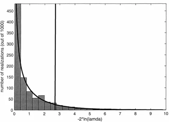
Lastly, the fact that the null hypothesis in (14) is known to be true provides an opportunity to demonstrate that - 2 ln(A) does in fact have a X2_{distribution with dim(Q)} -dim(Q2) degrees of freedom. Repetition of test (14) 1000 times with different

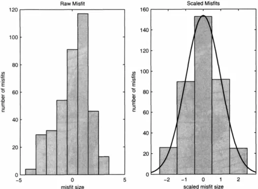
realizations of the generic linear data set in Fig. 1 produces the histogram of values of - 2 In(A) shown in Fig. 5. The %2 distribution (dark line) with 1 degree of freedom closely follows the histogram. As expected, 896 of the 1000 realizations fall below the 90% cumulative threshold, confirming the theoretical result. This figure also reiterates the rationale behind the m.l.r.t.: Since the behavior of X when the null hypothesis is true can be well approximated, the ability to reject a null hypothesis can be quantified based on departures from this expected behavior.

2.3 The Choice of a Misfit Probability Model and Implications for Misfit Weights

A probability distribution that adequately describes the statistical properties of the model/data misfit is critical to the validity of the analysis. This choice determines the misfit weights: if a misfit is improbable relative to the expectations of the error model, then it is weighted heavily. This choice can rarely be made on purely theoretical

grounds, and exploratory analysis, experience, and prior study often are required to refine the description. Although there are no steadfast rules to reference, Cox and Hinkley

(1974, pp. 4-5) offer the following guidelines that have been paraphrased:

1. The family of distributions should if possible establish a link with any theoretical knowledge about the system and with previous experimental work.

2. There should be consistency with known limiting behavior.

3. So far as possible, the parameters in the distribution should have clear-cut interpretations.

4. A family of distributions containing few parameters is preferable.

5. It is desirable for the statistical theory associated with the model to be as simple as possible.

The normal distribution is often justified on the grounds that, if the model misfit results from the sum of random noise from many different sources, the sum of these will be approximately normal by the central limit theorem. However, if the dominant misfit source is strongly non-normal, this logic can fail. Fortunately, various diagnostics are available to help determine if a particular choice of an misfit model is appropriate (e.g. Draper and Smith, 1981, Cook and Weisberg, 1982, D'Agostino and Stevens, 1986, Cuthbert and Wood, 1987). Such diagnostics are critical to resolving ambiguities in the best choice of weights (e.g. Evans, 2003).

Figure 6 (A-C) shows 3 simple diagnostic plots for the misfit of the example above. The histogram (panel A) shows that the misfits are largely symmetric about 0 and have tails consistent with the normal distribution, although there does seem to be a slightly higher than the expected number of large positive values. Panel B plots the residuals as a function of x, suggesting that the residual properties do not change as a

function of the independent variable. In the case of this simple example, invariance in x also implies invariance as a function of since the two are linearly related. Panel C shows a probability plot, which compares the ordered misfits (normalized by the

variance) to those expected based on the standard cumulative distribution function of the error model. If the misfits are consistent with the error model, the plot will form a

straight line. Curvature is indicative of discrepancies in the tails of the distribution or skewness. The plot in panel C is largely straight, despite a short increase in the slope associated with the slight prevalence of large positive values apparent in the histogram.

In the simple linear regression example, the diagnostic plots largely support the assumed misfit distribution. There is no strong asymmetry, no extreme outliers, and the width of the tails of the distribution is consistent. In deciding if the misfit model may require additional refinement, the appropriate question that must be asked is: are any refinements in the properties of the expected misfit distribution likely to materially change the conclusions of the study? If conclusions depended on very fine scale

delineations of the parameters in question, more exhaustive tests of the distribution may be required (see above references). However, in many cases a simple set of diagnostic plots such as those in Fig. 6, along with any additional plots with particular relevance to the problem at hand, should be sufficient to ensure the validity of the most prominent aspects of an analysis.

Lastly, it is notable that for many inverse modeling applications, setting the misfit variance before inversion is advocated (e.g. Bennett, 2002). The a-priori estimate of the misfit is included in the inversion and the model is optimized subject to physically realistic constraints on the initial conditions, boundary conditions, forcing, and model parameters. This fitting is most often carried out in a generalized least squares sense,

which produces maximum likelihood estimates for normally distributed noise. The primary hypothesis considered is if the model can match the observations within the expected achievable fit after adjusting controls within reasonable bounds (e.g. Muccino, et al., 2004). The same general machinery described herein is being applied in this case.

Setting the variance simply places more parameter restrictions for the null hypothesis in (8), and relationship (9) can still be used to identify parameter constraints based on the relative performance of the model with different parameter values. Likewise, the

a-posteriori estimates of the misfit produced in the example herein can be compared to any

available a-priori estimates of the achievable fit for comparisons similar to that described by Muccino et al. (2004). The choice of fixing the misfit variance a-priori or leaving it to estimation is a function of the scientific question being considered and the information available. If it is of primary interest to analyze the degree of fit after all known processes have been incorporated into the model, leaving the misfit to be estimated seems sensible. For either case, the parameter estimates will result from minimization of the unexplained variance between the model and the data.

3. Application of Maximum Likelihood Theory to Study HABs in the Gulf of Maine

The application of the methodology described above to test hypotheses regarding the initiation and development of blooms of the toxic dinoflagellate Alexandrium

fundyense in the western Gulf of Maine is now presented. Transition of the theory above

to application in a physical-biological model is challenging, and particular attention is paid to pragmatic decisions required to make this transition and the influence that these decisions have on the analysis. The section begins with a brief description of the observations and the formulation of the dynamics model. Steps taken to reduce the parameter space to a manageable dimension are then described, before proceeding to the misfit model formulation, hypothesis testing, and misfit model verification. The section concludes with a discussion of model assessment and diagnosis based on analysis results.

36

3.1 Observations and the Dynamics Model Formulation

Blooms of A. fundyense in the western Gulf of Maine (WGOM, Fig. 7) evolve within a dynamic physical and biological environment (Franks and Anderson, 1992a, Franks and Anderson, 1992b, Anderson, et al., 2004a). It is therefore hoped that a coupled physical biological model can lend insight into the factors controlling the timing and magnitude of the bloom beyond those that can be gleaned from the observations alone. A field program including 5 ship surveys (Fig. 8) and mooring deployments carried out in 1993 provides the observations for the study (Anderson, et al., 2004a, Geyer, et al., 2004). The duration of each survey was 2-3 days and they were spaced approximately 2 weeks apart (April 12-14, April 28-30, May 10-13, May 227, June 4-6). A. fundyense cell counts were taken at the surface (Fig. 8, top panel) and, for -75% of the stations, at 10 meters. Hydrographic and nutrient data, including phosphate, silicate, nitrate, nitrite, and ammonium (Martorano and Loder, 1997) was also collected (Fig. 8, bottom panel).

The physical component of the dynamics model is provided by the Estuarine, Coastal and Ocean Model (ECOM) (Blumberg and Mellor, 1987). The study domain (Fig. 7) is covered by a grid of 130 cells in the along-shore direction and 70 in the cross-shore. Grid cells dimensions range from 1.5-3 km. 12 sigma layers (i.e. each layer is a constant fraction of the water depth) are specified in vertical with increased resolution near the surface to better resolve river plume dynamics. Vertical mixing is calculated using the Mellor-Yamada level 2.5 turbulence closure (Mellor and Yamada, 1982, Galperin, et al., 1988). Model Forcing is summarized in Table 2, and was chosen to capture the principle aspects of the large-scale circulation and hydrography in the

WGOM (Chapters 3 and 4 of this thesis provide comparisons of the modeled circulation and data).

Alexandrium species are characterized by a life cycle that includes both a resting

cyst and a vegetative cell (Anderson, 1998). The transition between resting and vegetative stages occurs through the process of germination. The biological model is therefore a single component model constructed from laboratory-based parameterizations of A. fundyense germination, swimming behavior, and growth as functions of the

environmental conditions. The baseline model functions are summarized in Fig. 9, and the parameters are cataloged in Table 3. Detailed descriptions of the model construction can be found in Anderson et al. (submitted) and within the Appendix.

The baseline model structure provides the first null hypothesis. Additional structures are then considered in an effort to find the combination of parameters most capable of explaining the data (Table 4). The second structure adds the possibility of a spatially uniform averaged mortality (m), the third adds the possibility of a dependence of growth on dissolved inorganic nitrogen (DIN), while the fourth considers both mortality and nutrient dependence in combination. Mortality is loosely defined as a vegetative cell being removed from the water column (e.g. by grazing, formation of a new cyst, and/or

cell mortality). It is given a range to allow the possibility of negligible rates, to rates that would overwhelm all but the swiftest growth. The nutrient dependence is modeled using a Monod formulation with half-saturation constant KN.

,u(DIN, T, S) = t(T, S) x [DIN] (15)

KN + [DIN]

Where u is the growth rate and T and S are temperature and salinity respectively. The range of KN considered was chosen to encompass the range of half saturation constants

for nitrogen dependent growth and uptake commonly encountered in the literature (Table 3). These formulations are admittedly limited in their ability to recreate detailed

ecosystem dynamics. However, they do provide a means to test the necessity of a first-order mortality term and/or nutrient dependence in first-order to match the observed timing and magnitude of A. fundyense blooms.

3.2 Parameter Space Reduction

The coupled physical/biological model described above replaces the simple linear and quadratic dynamics models discussed in Section 2. This dynamics model can be viewed as an operator, A, that houses many parameter dependent relationships which eventually yield estimates of the cell abundance ( ):

y = A(O)+ e = + (16)

The parameter vector Onow contains all of the biological model parameters in Table 3, and all of the uncertain parameters in the physical model formulation (including the forcing). The misfit (e) is expected to arise from uncertainty in the observations, and

from dynamics that cannot be resolved deterministically by the physical and/or biological model.

Maximizing the likelihood over all , even for the relatively simple dynamics model described above, could quickly become computationally untenable without the employment of advanced techniques such as adjoint models (Lawson, et al., 1996, Spitz, et al., 1998). In addition, testing hypotheses concerning parameters with little influence or those with strong covariance with more dominant parameters will likely be a fruitless exercise, as the amount of independent information about the parameter within the observations is small. That is, the Fisher Information Matrix contains low values on the

diagonal associated with these parameters and/or high off-diagonal values associated with a second dominant parameter. The parameter space is therefore pared down by limiting it to those parameters most critical to the question of primary interest: what factors control the timing and magnitude of the observed bloom. In lieu of attempting an ad-hoc numerical approximation of I(0), a bulk sensitivity metric reflecting the degree that the uncertainties in Table 3 influence bloom magnitude is enlisted:

M(lfC(x, y, z,t)dxdydz₎

SM

(i, t),

(ffC(x, yLx zt)dxdydz

domain O = ,ow

Where C is the concentration of A. fundyense, 0,aigh is the value of the parameter under

consideration that is most favorable to cell abundance, and 6O,low is the value least favorable. Multiplied by 100, this metric yields the percentage change in the total

number of cells in the domain as a function of time (t) induced by varying each parameter over its approximate range of uncertainty. Two parameters clearly dominate this

uncertainty metric (Fig. 10). The germination depth (dg) dominates for the first 1.5 months of the simulation. This is the depth of sediment over which resting A. fundyense cells can germinate and gain the water column through the sediment grain matrix. Late in the simulation, the magnitude is most sensitive to the maximum growth rate, which can drive 10 fold changes by mid-may and nearly 100 fold changes by simulation's end.

Based on the strong dominance of dg and uAx demonstrated above, the free parameters within the baseline biological model are limited to these two, with model structures 2, 3, and 4 adding combinations of the uncertain parameters KN and m. The remaining baseline biological model parameters are given central values within their

uncertainty ranges. This transfers any unique observed patterns that these parameters could account for within their uncertainty into the misfit term (i.e. they are now in the null space of the dynamical model), and leaves the portions that covary with the dominant parameters to be compensated for by those parameters. While the former consequence simply increases the expected noise between model and data, the latter action risks the introduction of a bias to the estimates of dg, u ax, KN and m. For

example, if the true value of the growth efficiency ag is actually higher than the central value it is given, then the m.l.e. iman may compensate and tend to be higher than its true value. Reduction of the parameter space must be approached with caution for this reason. In the present case, the dominance of the remaining parameters is such that both the

additional noise and any potential bias introduced by the reduction are expected to be small.

The second assumption aiding in the reduction of the parameter space is that uncertainty of physical origin is small relative to uncertainty of biological origin.

Comparisons of the physical model with current meter data, surface salinity data, and surface temperature data all suggest that the primary features of the springtime evolution of WGOM river plumes, vernal warming, and the strength and direction of the coastal current are being captured (see Chapters 3 and 4). However, this step is as much justified by the large uncertainty in the biology (e.g. Fig. 10) as it is by the performance of the physical model. It is unlikely that even the most egregious physical errors could cause > 10 fold changes in bloom magnitude. If the misfits of physical origin persist over relatively small space/time scales and occur in a random manner (e.g. those stemming from the inability to deterministically simulate the exact placement and timing of

mesoscale phenomena), this physical noise will be manifest in an increase in the noise that will simply make hypotheses more difficult to reject (e.g. Fig. 4). However, conclusions will be tempered by recognition that any persistent bias in the physical dynamics, particularly in sensitive regions within the domain, could lead to bias in the estimates of biological model parameters.

3.3 Misfit Model Formulation

The reductions of the model parameter space described above allows the following simplification of (16):

y = A(u,, ,dg g ,KN,m)+ e = + E (18)

Although the same symbol has been used for the misfit as in (16), enow contains

contributions from the observational noise, unresolved physical and biological processes, any contributions from the imperfect physical model parameterization and forcing, as well as any misfit produced by setting the remaining biological model parameters to central values within their uncertainty. This diversity of misfit sources complicates the construction of a misfit model. Since the total misfit is the sum of many components that are at least partly independent, it could be argued that it would be approximately normal. However, the observations themselves vary over several orders of magnitude and the underlying dynamics (i.e. growth and mortality) are exponential in nature. This suggests that the log-transformed misfits may be normally distributed, which would grant

consistency in the weighting of misfits over orders of magnitude. The latter description will serve as the first misfit model guess.

An additional aspect of the dynamical model is that it was constructed in the hope of capturing the general timing and magnitude of bloom events, not their detailed

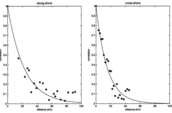
structure. It is thus expected that some covariance may exist between the misfits in both space and time. Inspection of the patch decorrelation scales (Fig. 11) in the along-shore and cross-shore directions suggests the possibility of an anisotropic spatial misfit

decorrelation. A misfit covariance matrix, Ce, is therefore included, where covariance decay is modeled with a simple function:

p,

Where rx and ry are exponential decay coefficients (kmn') in the cross-shore and alongshore directions respectively, Ax and Ay are the along-shore and cross-shore distances between any two points i, j, and 2_{is the misfit variance. The possibility of} temporal correlation is introduced with the factor p . The roughly equal bi-weekly spacing of the cruises makes it possible to use the number of cruises separating any two observations as a proxy for temporal lag. Thus, pa,= corresponds to the correlation between points at the same spatial location, but separated by 1 cruise. For points taken during the same cruise, this factor ( p,=0) has a value of 1. Only correlations between points separated by 1 or 2 cruises are considered herein. This simple representation of the covariance would likely be inadequate if, for example, the detailed dynamics across hydrodynamic fronts were being explored, but it should suffice for the goals of this analysis.

With this preliminary choice of misfit model, the likelihood can be written:

exp(- x e

CE)

L(O;e) =(2)nx

2

C )

Which is the N-dimensional joint normal distribution for a set of n misfits (e.g. Wunsch, 1996). Ois a vector consisting of the 4 free parameters in the biological model

(/, ,dg, ,KN , m) and 5 parameters in the misfit model (02, r , s , ,, p=2), and e is

the n x 1 vector of log-transformed model/data misfits:

Ei = ln(i + 1) -ln(y i + 1) (21)

One has been added to allow for the inclusion of 0 abundance observations in the analysis.

While an a-priori estimate of the misfit variance is not applied in the optimization directly, it is still useful to consider an expected level of fit. The goal of the analysis is to identify dynamics capable of recreating the timing and magnitude of the observed bloom. It is thus hoped that the model captures those portions of the data that are explained by the prominent, deterministically resolved aspects of the spring circulation combined with prominent seasonal patterns in the biological sources and sinks. Fig. 11 offers

information regarding how this level of agreement might translate to misfit variance. Much of the variability in the observations occurs over relatively short spatial scales (10-30 km), suggesting that small spatial displacements (that are acceptable to the goals of the analysis) will likely lead to large misfit variances. Recent data assimilative modeling efforts within the Gulf of Maine comparing the paths of modeled and observed drifters in the region just north of this domain (He, et al., submitted) show separations of this scale

are typical between 1 and 7 days after release despite considerable success at matching observed ADCP, mooring, and coastal sea level observations. It is not certain if the motions responsible for the separation in this particular set of drifters were random turbulent eddies or a persistent deterministic error in the flow field. However, if it is