HAL Id: hal-01730257
https://hal.archives-ouvertes.fr/hal-01730257
Submitted on 13 Mar 2018
HAL is a multi-disciplinary open access
archive for the deposit and dissemination of
sci-entific research documents, whether they are
pub-lished or not. The documents may come from
teaching and research institutions in France or
abroad, or from public or private research centers.
L’archive ouverte pluridisciplinaire HAL, est
destinée au dépôt et à la diffusion de documents
scientifiques de niveau recherche, publiés ou non,
émanant des établissements d’enseignement et de
recherche français ou étrangers, des laboratoires
publics ou privés.
Magnetic field continuity conditions in finite-element
analysis
Yvan Lefèvre, Carole Hénaux, Jean-François Llibre
To cite this version:
Yvan Lefèvre, Carole Hénaux, Jean-François Llibre. Magnetic field continuity conditions in
finite-element analysis. IEEE Transactions on Magnetics, Institute of Electrical and Electronics Engineers,
2018, 54 (3), pp.7400304. �10.1109/TMAG.2017.2762084�. �hal-01730257�
O
pen
A
rchive
T
OULOUSE
A
rchive
O
uverte (
OATAO
)
OATAO is an open access repository that collects the work of Toulouse researchers and
makes it freely available over the web where possible.
This is an author-deposited version published in :
http://oatao.univ-toulouse.fr/
Eprints ID : 19669
To link to this article : DOI:10.1109/TMAG.2017.2762084
URL :
http://dx.doi.org/10.1109/TMAG.2017.2762084
To cite this version :
Lefèvre, Yvan and Henaux, Carole and Llibre,
Jean-François Magnetic field continuity conditions in finite-element
analysis. (2018) IEEE Transactions on Magnetics, vol. 54 (n° 3). pp.
7400304/1-7400304/4. ISSN 0018-9464
Any correspondence concerning this service should be sent to the repository
administrator:
[email protected]
Magnetic Field Continuity Conditions in Finite-Element Analysis
Y. Lefevre , C. Henaux, and J. F. Llibre
LAPLACE, University of Toulouse—CNRS, Toulouse, 31071 France
This paper deals with the magnetic field continuity conditions in finite-element analysis. Our study is based on numerical and analytical models. Different known finite-element codes, based on 2-D nodal finite element or 3-D edge element, are used to analyze the magnetic field in a linear motor-like device. The use of an analytical model gives interesting insight on interface errors problems in finite-element analysis.
Index Terms— Analytical model, edge element, magnetic devices, magnetic fields, nodal finite element.
I. INTRODUCTION
T
HE normal component of the magnetic flux density B andthe tangential component of the magnetic field strength H satisfy the field continuity conditions at the interface of two media of different permeability values. It has been known that in finite-element method (FEM) there are interface error problems due to the fact that only one continuity condition is imposed strongly by FEM [1], [2]. This paper analyses in a simple device these interface error problems. As most of applications required only a 2-D numerical calculation, we will use first 2-D nodal FEM. In some applications, as in axial flux motor, 3-D numerical calculation is needed. The 3-D edge FEM will be used. Edge elements have been developed to overcome some drawbacks of 3-D nodal finite element [3]. First, the studied device is presented. Then the study of the interface error problems on our simple device is performed with different numerical models. Eventually, analytical model is used to theoretically analyze the results obtained.II. STUDIEDSLOTLESSDEVICE ANDFEM
COMPUTATIONS
A. Slotless Device
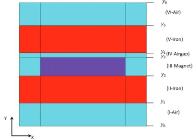
In order to quantify interface errors, the distribution of magnetic field inside a permanent magnet linear motor-like device is analyzed. The geometry of the motor is very simple. Fig. 1 shows a pole pitch of this device. It is easy to see where the permanent magnet and airgap are.
Above the airgap is the upper plate made of iron and under the permanent magnet is the bottom plate made also of iron. Above the upper plate and under the bottom plates there is air. The permanent magnet is polarized in the vertical axis (Oy). The axis (Ox) is horizontal. A slotless motor-like device is chosen in order to avoid corner effects that may affect the analyses.
Table I gives the geometric and physical parameters.
Color versions of one or more of the figures in this paper are available online at http://ieeexplore.ieee.org.
Digital Object Identifier 10.1109/TMAG.2017.2762084
Fig. 1. Studied device: in red iron, in dark blue the permanent magnet polarized parallel to the vertical axis (Oy) and in light blue the air region.
TABLE I
PARAMETERS OF THELINEARMOTORLIKEDEVICE
B. Study Domain
The geometry of the pole pitch is supposed to be repeated alternately in the horizontal direction (Ox). The pole pitch is composed of six isotropic and homogeneous regions (Fig. 1). The regions are numbered consecutively along the vertical axis (Oy): the lowest and mots upper are named as Region I and Region VI. Each region k is bounded by two planes with y constant (yk−1, yk). The regions numbered I and VI are air regions and they span to infinity in the vertical direction (Oy): y0 tends to minus infinity and y6 to infinity. Regions
num-bered II and V are iron regions. Region III corresponds to the magnet region and region IV is the airgap. Tangential magnetic field is imposed on the bottom and upper lines and the magnetic field is anti-cyclic along Ox.
Fig. 2. FEMM 2-D mesh with first-order triangular element.
Fig. 3. ANSYS Emag 2-D mesh with quadrangular elements.
C. Meshes Used for 2-D Nodal FEM and 3-D Edge FEM Two different FEM software have been used. The first one is finite element method magnetics (FEMM) which is a software package that can be downloaded from internet [4]. Fig. 2 shows a 2-D mesh with a first-order triangular element with 14557 elements and 7377 nodes obtained from FEMM. It can be seen the mesh in the airgap is very fine.
The second software is ANSYS Emag [5], [6]. Two different 2-D meshes with 3420 quadrangular elements have been performed.
The mesh with first-order element has 3565 nodes and the one with second-order element 10549 nodes (Fig. 3). The last mesh obtained with ANSYS Emag is a 3-D mesh with 62016 hexahedral edge elements (Fig. 4).
D. Distribution of Ht Along the Interface Iron Side
In 2-D, a nodal vector potential formulation is used and in 3-D, an edge element vector potential [3]–[6]. In both cases, the continuity of Htis not imposed. The theory guarantees that if the number of nodes increases the gap between the values of Ht at each side of the interface decreases [1]–[3]. As the continuity of Bn is guaranteed, only the continuity of Ht is studied here. The distribution of Ht along the interface has
Fig. 4. ANSYS Emag 3-D mesh with hexahedral egde element.
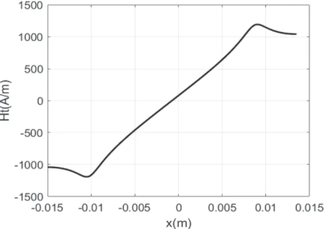
Fig. 5. Distribution of Ht, along the interface (y = y4) and in the plane
parallel to (x Oy) on the middle of the z-axis, calculated iron side.
been calculated by different finite-element codes with different meshes. Only some results are shown here.
The results obtained using the nodes and elements of the iron side do not change with the type of element, 2-D or 3-D, triangular or quadrangular, nor the order of approximation, first order or second order (Fig. 5).
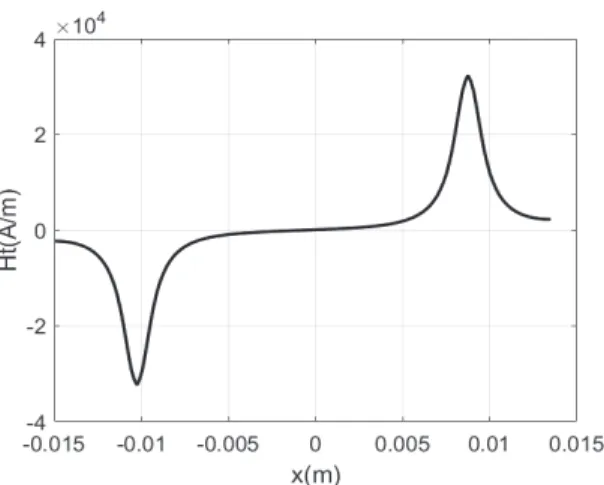
E. Distribution of Ht Along the Interface Airgap Side The distribution of Ht airgap side, calculated from nodes and elements of the airgap, with 2-D first-order element is very different from the distribution calculated in the iron side. It does not change very much with the type of ele-ment, triangular, or quadrangular (Fig. 6). A huge gap is observed between the two distributions of Ht along the interface (Figs. 5 and 6).
The distribution of Ht on the interface has been also calculated by means of a 3-D edge element model. It is quite similar that one on Fig. 6.
The Ht distribution in the airgap side obtained from second-order element is not very different from the distribution calculated in the iron side (Fig. 7). The gap of Ht on both sides is very much reduced but it is worth to recall that the second-order mesh has threefold of nodes (10549 nodes) than
Fig. 6. Distribution of Ht, along the interface (y = y4) and in the plane
parallel to (x Oy) on the middle of the z-axis, calculated airgap side.
Fig. 7. Distributions of Ht, along the interface (y = y4) and in the plane
parallel to (x Oy) on the middle of the z-axis, calculated in the airgap and iron sides with 2-D second-order quadrangular elements.
the first-order mesh (3565 nodes) which is already a very dense mesh.
We can notice ripples on the distribution calculated by second-order element. This result confirms that the gap between the two values of Ht on both side decreases when the number of nodes increases.
Furthermore, if the distribution in airgap side is not calcu-lated exactly on the interface but, for instance, at a distance of about one-tenth of the thickness of the airgap (see Table I), the distribution shown in Fig. 6 is obtained again. In the same way, the distribution observed in Fig. 5 does not change at all in the iron.
III. ANALYTICALMODEL OFSLOTLESSDEVICE
The geometry of this device, shown in Fig. 1, is very simple and a 2-D analytical model of the field distribution can be developed. Generally in such analytical models the magnetic core is assumed to have infinite permeability and only the regions having the permeability of air are considered [7]. Nevertheless, in this paper the continuity conditions between two regions of different permeabilities are taken into account and then the assumption of infinite permeability is not made.
In each region, the magnetic field density B and magnetic field intensity H are linked (2)
B =µH + JP (1)
where JPis the magnetic polarization and µ is the permeability
of the material. JPis null vector except in the magnet and has
only one component along the vertical (Oy) axis.
As the problem can be assumed to be invariant along the (Oz) axis, the vector potential A has only one non-null component along this axis. The vector potential is governed by a Poisson’s equation ∂2A ∂x2 + ∂2A ∂ y2 = − ∂JP ∂x . (2) Considering the symmetry of the device, the non-null com-ponent JP of the polarization of magnet varies only in the horizontal direction (Ox) and can be expressed as a Fourier series [8] JP(x , y) = ∞ % n=1,3,5,7,... Jnsin(nλx) Jn= 4JM nπ sin(nλwa) and λ = π wp . (3)
In (3), wp and wa are, respectively, the width of the pole pitch and the width of the magnet in (Ox) direction. In each region k, the solution of Laplace or Poisson’s equation (6) can be expressed in Fourier series [7]
A(k)(x , y) = ∞ % n=1,3,5,7,... A(k)n (y)sin(nλx)
A(k)n (y) = Cn(k)enλy+D(k)n e−nλy− Jn(k)
nλ .
(4)
In (6), Jn(k) is null in all regions except region III. The constants Cn(k)and Dn(k)are determined by boundary conditions and continuity conditions at each interface. When y tends to minus infinity or to infinity the vector potential is null so coefficientsD(1)n and Cn(6) are equal to zero. For each harmonic n, the ten left constants are determined by the continuity conditions on each interface yk, k = 1, 2, . . . , 5. The continuity of Bn and Ht on these interfaces give the ten equations ∂ A(k)(x , yk) ∂ x = ∂ A(k+1)(x , yk) ∂ x 1 µk ∂ A(k)(x , y k) ∂ y = 1 µk+1 ∂ A(k+1)(x ,yk) ∂ y . (5)
The distributions of Ht along lines parallel to (Ox) have been calculated by means of the proposed analytical model. Four lines in the airgap and four in region V iron have been defined in order to show how the Ht distributions along lines parallel to (Ox) vary. These lines Li are defined as follows:
Li :y = y4−2(i − 1)δy. (6) For the lines in the airgap, δy is chosen equal to the thick-ness of airgap (1 mm) divided by 1000. For the lines in region V, δy is negative and is equal to the thickness of the “stator” (6 mm) divided by 20. So in the airgap the four lines
Fig. 8. Distributions of Ht along lines L1, L2, L3, and L4in the airgap
(δy = 1 µm).
Fig. 9. Distributions of Ht along lines L1, L2, L3, and L4 in iron
(δy = 300 µm).
are very close to each other compared to the four lines in region V. The first of these lines L1 is, in each case, the
interface between airgap and region V.
In Figs. 8 and 9, the origin of x-axis is on the middle of the interface. In Figs. 5 to 7 the origin of x-axis is at the left side of the study domain (Fig. 1)
The distributions of Ht along lines in the airgap are shown in Fig. 8. Knowing that the lines are very close, Fig. 8 shows that Htvaries strongly in function of the vertical coordinate y. Note that the distribution on L1has the lowest variation.
The distributions of Ht along lines in iron are shown in Fig. 9. In this case, the distance between lines is much greater than the distance between lines in the airgap. Fig. 9 shows that Ht varies slowly in function of y in region V. The distribution on L1is the highest one.
It is important to note that the distributions of Htjust on the interface, line L1, in Figs. 8 and 9 are the same. This result
was expected because the analytical model imposes, by (7), the continuity of Ht on interface.
The results obtained from the analytical model show first that the variation of Ht as a function of y in the airgap is very strong and almost exponential according to (6). This variation is hardly described by FEM if first-order elements are used. It can explain why the computation of electromagnetic forces and torques regularly leads to uncertain results that are strongly dependent on the applied mesh [8], [9]. It is also worth noting that the distribution calculated analytically on the interface (L1) is the distribution calculated iron side by
finite-element analysis (Fig. 5).
IV. CONCLUSION
Theoretical considerations on FEM lead to the conclusion that interface errors are inherent to the weak formulation used in FEM. Gaps on interface are observed with 2-D nodal first-order finite element and 3-D edge element. An analytical model of the magnetic field shows that the variation of the tan-gential component of magnetic field strength with the distance from the iron-airgap interface is so strong that first-order finite element may hardly succeed to account of it. Better results are obtained with second-order 2-D nodal finite element. For this simple example without corners, the distribution calculated by finite-element iron side gives always the distribution on the interface calculated analytically.
REFERENCES
[1] A. Bossavit, “How weak is the ‘weak solution’ in finite element methods?” IEEE Trans. Magn., vol. 34, no. 5, pp. 2429–2432, Sep. 1998. [2] K. Reichert, R. E. Neubauer, and T. Tarnhuvud, “A new approach solving the interface error problem of finite element field calculation methods by means of fictitious interface current sheets or interface charges,” IEEE
Trans. Magn., vol. 28, no. 2, pp. 1696–1699, Mar. 1992.
[3] J. Jin, The Finite Element Method in Electromagnetics, 2nd ed. Hoboken, NJ, USA: Wiley, Jun. 2002.
[4] D. Meeker, “Finite element method magnetics—Version 4.0 user’s manual,” Univ. of Virginia, Charlottesville, VA, USA, Tech. Rep., 2004. [Online]. Available: http://www.femm.info/Archives/doc/manual42.pdf [5] “2-D static magnetic analysis,” in ANSYS Mechanical APDL Low
Frequency Electromagnetic Analysis Guide. Release 17.2, ch. 2, Aug. 2016.
[6] “3-D magnetostatics and fundamentals of edge-based analysis,” in
ANSYS Mechanical APDL Low Frequency Electromagnetic Analysis Guide. Release 17.2, ch. 6, Aug. 2016.
[7] K. Boughrara, B. L. Chikouche, R. Ibtiouen, D. Žarko, and O. Touhami, “Analytical model of slotted air-gap surface mounted permanent-magnet synchronous motor with magnet bars magnetized in the shifting direc-tion,” IEEE Trans. Magn., vol. 45, no. 2, pp. 747–758, Feb. 2009. [8] R. Castillo and J. M. Cañedo, “A 2D finite-element formulation for
unambiguous torque calculation,” IEEE Trans. Magn., vol. 44, no. 3, pp. 373–376, Mar. 2008.
[9] T. T. Overboom, J. P. C. Smeets, J. W. Jansen, and E. A. Lomonova, “Semianalytical calculation of the torque in a linear permanent-magnet motor with finite yoke length,” IEEE Trans. Magn., vol. 48, no. 11, pp. 3575–3578, Nov. 2012.