HAL Id: hal-03012944
https://hal.archives-ouvertes.fr/hal-03012944
Submitted on 18 Nov 2020
HAL is a multi-disciplinary open access
archive for the deposit and dissemination of
sci-entific research documents, whether they are
pub-lished or not. The documents may come from
teaching and research institutions in France or
abroad, or from public or private research centers.
L’archive ouverte pluridisciplinaire HAL, est
destinée au dépôt et à la diffusion de documents
scientifiques de niveau recherche, publiés ou non,
émanant des établissements d’enseignement et de
recherche français ou étrangers, des laboratoires
publics ou privés.
Magnet Shape
Théo Carpi, Yvan Lefèvre, Carole Hénaux, Jean-François Llibre, Dominique
Harribey
To cite this version:
Théo Carpi, Yvan Lefèvre, Carole Hénaux, Jean-François Llibre, Dominique Harribey. 3D Hybrid
Model of the Axial Flux Motor Accounting Magnet Shape. IEEE Transactions on Magnetics, Institute
of Electrical and Electronics Engineers, 2020, pp.1-1. �10.1109/TMAG.2019.2950892�. �hal-03012944�
3D Hybrid Model of the Axial Flux Motor Accounting Magnet Shape
T. Carpi, Y. Lefèvre, C. Hénaux, J.F. Llibre and D. Harribey
Laboratoire Plasma et Conversion d’Energie (LAPLACE), University of Toulouse, CNRS, 31000 Toulouse, France
This paper presents a generalization of an analytical model of an axial flux permanent magnet machine to any magnet shape. It uses an existing model which computes the 3D magnetic flux density by the separation of variables and finite difference method. The original magnet shape is modified by adding a radial dependency to the Fourier series description of permanent magnets magnetization. The model is then developed for a general complex magnet shape. As an example, the model will be computed for a circular magnet shape and will be compared to a finite element analysis.
Index Terms— Axial flux, finite difference method, Fourier series, magnetic scalar potential, magnet shape, permanent magnet,
separation of variables.
I. INTRODUCTION
HE structures of Axial Flux Permanent Magnet (AFPM) machine structures are still under development [1]. Thus, modeling some of their particularities is becoming an issue. In axial flux surface mounted permanent magnet machines, permanent magnets are often considered as sector shaped magnets. However, others magnet shapes can be found in some AFPM structures [1], [2], [3]. Nevertheless, considering 3D analytical modeling, despite the variety of the methods used, only sector shaped magnets have been considered [4], [5], [6].
The method developed in [6] consists in a combined resolution with analytical and finite difference method (FDM). The resolution is based on the image method where the geometry is repeated infinitely in the axial direction [5]. This way, the problem can be described by a double Fourier series in the axial and angular directions. The Laplacian is then solved by separation of variables. However, Bessel functions given for the radial solutions are not chosen because of their complexity. Instead, the r dependent function is kept unknown and solved by a 1D FDM.
This model is adaptable to any magnets distributions thanks to the Fourier series description. It is also adaptable to multistage machines thanks to the image method. Nevertheless, only sector shaped magnets can be modeled by this method. Benefiting from the FDM in the radial direction, this paper proposes to extend the model to any magnet shapes by modifying the Fourier series description for each discretized radius. Subsequently, the solution will be computed for circular magnet shape and compared to finite element analysis (FEA).
II. GENERALIZATION OF THE MAGNET SHAPE
A single sided AFPM machine with axially magnetized surface mounted permanent magnets is considered in this paper.
As in [6], the following assumptions are made:
- Because of the air-space between the magnets, we assume that the permeability of magnets and the air is the same and equal to µ0.
- Back-irons have infinite permeability so the boundary conditions (BC) at the planes z = 0 and z = hm + g is taken as
normal flux boundary conditions. Where g is the airgap width and hm the permanent magnet width.
- The problem is limited in the radial direction with parallel flux boundary conditions on cylinders at r = R0 and r = R1.
Using magnetic scalar potential formulation (MSP), Ω, the partial differential equation to be solved is deduced from Maxwell equations:
∆Ω = 𝑑𝑖𝑣 𝑴 (1) with M the magnetization vector.
To reduce the number of regions to consider, the image method is used to replace the normal flux BC by a periodical extension in the axial direction [6]. This leads to a double Fourier series description of the magnetization of the permanent magnets in the azimuthal θ and axial z directions.
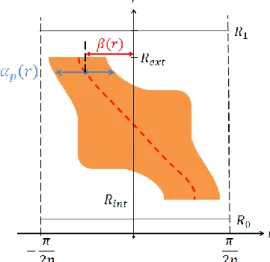
A complex magnet shape is considered in Fig. 1. To be able to compute this magnet shape, the Fourier series description has to be modified depending on the radial position. The parameters necessary to characterize any shape are the arc pole αp and the phase β between the origin and the center
position of the angular opening as shown in Fig. 1. Thus, a general Fourier series describing the magnetization Mz of any
magnet shape can be expressed as follows. 𝑀𝑧(𝑟, 𝜃, 𝑧) = ∑ 𝑛 ∑ 𝑀𝑛𝑘(𝑟) cos(𝑛𝑝𝜃 + 𝛽(𝑟)) cos (𝑘𝜋𝜏 𝑧) 𝑘 (2) where p is the number of pole pairs, τ = hm+g is the half period
of the magnetization in the z-direction.
Fig. 1. Complex magnet shapes with the arc pole and the phase depending on radial position.
The coefficients Mnk have to be determined in function of
αp(r) and the phase β(r) which represents purely the
asymmetrical feature of the magnet shape. Fig. 2 shows the angular and axial dependency of the magnetization for a given radius. The image method repeats the geometry in the axial direction, so Mz(z) is not impacted by the magnet shape.
Fig. 2. Angular (a) and axial (b) dependency of the magnetization.
III. HYBRID MODELING METHOD
Thanks to the double Fourier series description, there are three regions to be considered separated by cylindrical surfaces at r = Rint and r = Rext. Air regions I (Rint ≥ r ≥ R0) and
III (R1 ≥ r ≥ Rext), and the PM region II (Rext ≥ r ≥ Rint). The
new magnet shape must be included in the magnet region between Rint and Rext.
Fig. 3. Representation of the different regions considered in the problem.
In order to make the solution easier to handle, the Fourier series of the magnetization (2) is written in terms of cosine and sine functions.
𝑀𝑧(𝑟, 𝜃, 𝑧) = ∑ 𝑛 ∑ 𝑀𝑐𝑛𝑘(𝑟) cos(𝑛𝑝𝜃) cos (𝑘𝜋 𝜏 𝑧) 𝑘 + ∑ 𝑛 ∑ 𝑀𝑠𝑛𝑘(𝑟) sin(𝑛𝑝𝜃) cos (𝑘𝜋 𝜏 𝑧) 𝑘 (3) All the magnets are axially magnetized. Therefore, the magnetization 𝑴 has only a component in the axial direction. The second member of the equation (1) is reduced to:
𝜕𝑀𝑧 𝜕𝑧 = ∑ 𝑛 ∑ −𝑘𝜋 𝜏 𝑀𝑐𝑛𝑘(𝑟)cos(𝑛𝑝𝜃)sin( 𝑘𝜋 𝜏 𝑧) 𝑘 + ∑ 𝑛 ∑ −𝑘𝜋𝜏 𝑀𝑠𝑛𝑘(𝑟)sin(𝑛𝑝𝜃)sin(𝑘𝜋 𝜏𝑧) 𝑘 (4)
The separation of variables consists in assuming that the solution Ω is the product of three functions f, g and h:
Ω(𝑟, 𝜃, 𝑧) = 𝑓(𝑟). 𝑔(𝜃). ℎ(𝑧) (5) Combining (1) and (5) leads to three ordinary differential equations for each function f, g and h. The solutions for f are Bessel functions and cosine and sine functions both for h and g. To avoid using Bessel functions, f is kept unknown and will be determined by FD method. The principle of superposition allows writing the solution as follows:
Ω(𝑟, 𝜃, 𝑧) = ∑ ∞ 𝑛 ∑ 𝜔𝑐𝑛𝑘(𝑟) cos(𝑛𝑝𝜃) sin (𝑘𝜋 𝜏 𝑧) ∞ 𝑘 + ∑ ∞ 𝑛 ∑ 𝜔𝑠𝑛𝑘(𝑟) sin(𝑛𝑝𝜃) sin (𝑘𝜋 𝜏 𝑧) ∞ 𝑘 (6) The function f is now replaced by ωcnk and ωsnk which
depend on the harmonic rank, np and kπ/τ are respectively the periodicities in the angular and axial direction. Thus, inserting (6) in the partial differential equation (1) yields to three ordinary differential equations in each region I, II and III over the new unknowns ωcnk and ωsnk.
{ 𝑑2𝜔 𝑐𝑛𝑘𝐼 𝑑𝑟2 + 1 𝑟 𝑑𝜔𝑐𝑛𝑘𝐼 𝑑𝑟 − ( 𝑘2𝜋2 𝜏2 + 𝑛2𝑝2 𝑟2 ) 𝜔𝑐𝑛𝑘𝐼= 0 𝑑2𝜔 𝑐𝑛𝑘𝐼𝐼 𝑑𝑟2 + 1 𝑟 𝑑𝜔𝑐𝑛𝑘𝐼𝐼 𝑑𝑟 − ( 𝑘2𝜋2 𝜏2 + 𝑛2𝑝2 𝑟2 ) 𝜔𝑐𝑛𝑘𝐼𝐼= −𝑀𝑐𝑛𝑘 𝑘𝜋 𝜏 𝑑2𝜔 𝑐𝑛𝑘𝐼𝐼𝐼 𝑑𝑟2 + 1 𝑟 𝑑𝜔𝑐𝑛𝑘𝐼𝐼𝐼 𝑑𝑟 − ( 𝑘2𝜋2 𝜏2 + 𝑛2𝑝2 𝑟2 ) 𝜔𝑐𝑛𝑘𝐼𝐼𝐼= 0 (7) { 𝑑2𝜔 𝑠𝑛𝑘𝐼 𝑑𝑟2 + 1 𝑟 𝑑𝜔𝑠𝑛𝑘𝐼 𝑑𝑟 − ( 𝑘2𝜋2 𝜏2 + 𝑛2𝑝2 𝑟2 ) 𝜔𝑠𝑛𝑘𝐼= 0 𝑑2𝜔 𝑠𝑛𝑘𝐼𝐼 𝑑𝑟2 + 1 𝑟 𝑑𝜔𝑠𝑛𝑘𝐼𝐼 𝑑𝑟 − ( 𝑘2𝜋2 𝜏2 + 𝑛2𝑝2 𝑟2 ) 𝜔𝑠𝑛𝑘𝐼𝐼= −𝑀𝑠𝑛𝑘 𝑘𝜋 𝜏 𝑑2𝜔 𝑠𝑛𝑘𝐼𝐼𝐼 𝑑𝑟2 + 1 𝑟 𝑑𝜔𝑠𝑛𝑘𝐼𝐼𝐼 𝑑𝑟 − ( 𝑘2𝜋2 𝜏2 + 𝑛2𝑝2 𝑟2 ) 𝜔𝑠𝑛𝑘𝐼𝐼𝐼= 0 (8)
There are n x k equations to be solved in each region and for each cosine and sine component.
The boundary conditions (9) and (10) over the cylinders r = R0 and r = R1 are taken as parallel flux so that no flux goes out
of the region:
𝐵𝑟𝐼| 𝑟=𝑅0= 0 (9)
𝐵𝑟𝐼𝐼𝐼| 𝑟=𝑅1= 0 (10)
The interface conditions (11) to (16) between the permanent magnet region II and the air regions (I and III) over the cylinders r = Rint and r = Rext are the continuity of the normal
component of the magnet flux density Bn and the continuity of
the tangential component of the magnetic field density Ht:
𝐵𝑟𝐼| 𝑟=𝑅𝑖𝑛𝑡= 𝐵𝑟 𝐼𝐼| 𝑟=𝑅𝑖𝑛𝑡 (11) 𝐻𝜃𝐼| 𝑟=𝑅𝑖𝑛𝑡=𝐻𝜃 𝐼𝐼| 𝑟=𝑅𝑖𝑛𝑡 (12) 𝐻𝑧𝐼| 𝑟=𝑅𝑖𝑛𝑡=𝐻𝑧𝐼𝐼| 𝑟=𝑅𝑖𝑛𝑡 (13)
𝐵𝑟𝐼𝐼| 𝑟=𝑅𝑒𝑥𝑡=𝐵𝑟 𝐼𝐼𝐼| 𝑟=𝑅𝑒𝑥𝑡 (14) 𝐻𝜃𝐼| 𝑟=𝑅𝑒𝑥𝑡=𝐻𝜃 𝐼𝐼| 𝑟=𝑅𝑒𝑥𝑡 (15) 𝐻𝑧𝐼| 𝑟=𝑅𝑒𝑥𝑡=𝐻𝑧𝐼𝐼| 𝑟=𝑅𝑒𝑥𝑡 (16)
Continuity of the tangential component of the magnetic field density Ht leads to the continuity of the functions ωcnk
and ωsnk, while the continuity of the normal component of the
magnetic flux density Br yields to the continuity of ∂ωcnk/∂r
and ∂ωsnk/∂r.
Adding the interface and boundary conditions bring about a matrix system for each harmonic rank gathering all equations mentioned before:
𝐴𝑐𝑛𝑘. 𝑣𝑐𝑛𝑘= 𝐵𝑐𝑛𝑘 (17) 𝐴𝑠𝑛𝑘. 𝑣𝑠𝑛𝑘= 𝐵𝑠𝑛𝑘 (18) The final expression of the axial magnetic flux density is deduced from the magnetic scalar potential solved by FD method: 𝐵𝑧= −𝜇0[∑ ∞ 𝑛 ∑ 𝑣𝑐𝑛𝑘. cos(𝑛𝑝𝜃) .𝑘𝜋 𝜏 . cos ( 𝑘𝜋 𝜏 𝑧) ∞ 𝑘 + ∑ ∞ 𝑛 ∑ 𝑣𝑠𝑛𝑘. sin(𝑛𝑝𝜃) .𝑘𝜋 𝜏 . cos ( 𝑘𝜋 𝜏 𝑧) ∞ 𝑘 + 𝑀𝑧(𝑟, 𝜃, 𝑧)] (19)
where vnk are functions of 𝑟. Differential equations are solved
by FD method for each azimuthal n and axial k harmonics. The 1D FD method discretizes the problem in the radial direction and is continuous in the angular and axial directions thanks to the Fourier series description. The general method for any magnet shape was presented. In the next section, this model is applied to cylindrical magnet shape as an example.
IV. CIRCULAR MAGNET SHAPE
The model is applied to an AFPM machine with cylindrical magnets as shown in Fig. 4 and its parameters are given in Table 1. This magnet shape is often used in AFPM machines [1]. Thanks to the symmetrical shape of this type of magnet, the phase β(r)=0 and the Fourier series of the magnetization Mz is reduced to (20). 𝑀𝑧(𝑟, 𝜃, 𝑧) = ∑ ∞ 𝑛=1,3,5 ∑ 𝑀𝑛𝑘(𝑟) cos(𝑛𝑝𝜃) . cos (𝑘𝜋𝜏 𝑧) ∞ 𝑘=1 + ∑ 𝑀𝑛0(𝑟) cos(𝑛𝑝𝜃) ∞ 𝑛=1,3,5 (20)
Fig. 4. 3-D view of the AFPM machine with circular magnets.
TABLEI
PARAMETERS OF THE AFPMMACHINE
Parameter Value Magnetization (Remanence) (BM r) 1.026 MA/m (1.29 T) Magnet height hm 5 mm Airgap height g 6 mm Minimum radius R0 10 mm Maximum radius R1 32 mm
Magnet center radial position Rc 21 mm
Magnets radius R 7.5 mm Pole pairs number p 4
Mnk and Mn0 are the Fourier series coefficients:
𝑀𝑛𝑘(𝑟) = 8 𝑀 𝑛𝑘𝜋2sin (𝑘𝜋 ℎ𝑚 𝜏 ) sin ( 𝑛𝛼𝑝(𝑟)𝜋 2 ) (21) 𝑀𝑛0(𝑟) = ℎ𝑚 𝜏 4𝑀 𝑛𝜋sin ( 𝑛𝛼𝑝(𝑟)𝜋 2 ) (22) For each discretized radius r, the arc pole is calculated in order to create a circular shape.The arc pole expression is deduced from Fig. 5 (a):
𝛼𝑝(𝑟) = (𝑎𝑐𝑜𝑠𝑅𝑐 2+ 𝑟2− 𝑅2 2. 𝑅𝑐. 𝑟 ) 𝜋 2𝑝 ⁄ (23) As seen in Fig. 4, Rc is the radial position of the center of
the magnet and R the radius of the circular magnet. This allows creating an exact circular shape from the initial sector shape. The arc pole function is plotted in Fig. 5 (b).
The FEA is carried out on ANSYS/Emag 3D [7] and based on a magnetic scalar potential formulation. The FEA is done under the same condition as the model, that means on one pair of poles of the machine. Also, the same assumptions are made: the permeability of the magnets and BC.
To validate the fact that the magnet shape has changed, both computation methods are compared on a radial line at the middle of the airgap z = hm + g/2 and for several angles θ = 0°
(in front of the symmetrical axis), θ = 5.5° and θ = 7.5°. The results are computed for 16 harmonics. The root mean square (RMS) error between the hybrid model and the FEA on Fig. 6 are about 1.2% for the three plots.
Fig. 5. Modification of magnets shape (a) and arc pole in function of the radius (b).
Fig. 6. Axial flux density as a function of the radial coordinate computed by hybrid analytical-FD method and FEA.
The RMS errors are about 1.2% and 0.6% if we consider the influence of θ and z independently.
Back electromotive force and torque can be easily comput-ed from the Bz component of the magnetic flux density [6]. If
the field created by eddy currents may be neglected, eddy current losses in the magnets can be estimated. The armature reaction field must be computed. The laplacian can be solved in 2D (𝜃, 𝑧) using a MSP formulation [8]. Removing the magnets from this study and adding the boundary condition 𝐻𝑡= 𝐾 at the interface with the stator (𝑧 = ℎ𝑚+ 𝑔), where 𝐾
is the current sheet modeling the winding distribution, allows to solve the problem. Then, the same method used to calculate eddy current losses in [8] can be applied.
V. ACCURACY AND COMPUTATION TIME
The results of the hybrid model presented Fig. 6 are computed for 1) FDM part of the model: a radial discretization of 141 points and n and k equals 16 harmonics 2) analytical part of the model: 91 points and 221 points respectively for the angular and axial discretization. The total number of nodes is then 2,087,787 in the volume considered.
The computer used for the simulation is an Intel Core i7 at 1.9 GHz and 32 Go RAM. The computation time for 16 harmonics is 40 seconds to generate the entire solution. Nevertheless, the purpose here was to validate the model, so the computation time might be optimized. The addition of the radial dependency of the arc pole includes a loop into several initial nested loops, generating an increase of the computation time. It is approximately 4 times bigger than the one in [6], but remains much less than a FEA that took 74 seconds for 83,302 nodes within the same volume.
Fig. 7 presents the accuracy of the model and the computation time with respect to the number of harmonics. The RMS error mentioned above are the errors in the r-direction for z = hm + g/2 and θ = 0, θ-direction for r = Rint +
0.8(Rext-Rint) and z = hm + g/2 and z-direction for r = Rint +
0.8(Rext-Rint) and θ = 0. Therefore, a good accuracy can be
reached with a small number of harmonics, and the computation time is convenient to include the model into optimization studies for example. Thus, this model presents the advantage of being faster, easy to set up, and offering larger perspectives over the usual FEA.
Fig. 7. Accuracy and computation time in function of the number of harmonics.
VI. CONCLUSION
This paper presents a generalization of a 3D analytical model of AFPM with sector shaped magnets to AFPM with more complex magnet shapes. The method consists in including a radial dependency to the Fourier series description of the magnetization to be able to compute any magnets shape. The model was developed for a general complex magnet shape and the specific case of circular magnet shape was taken as an example, the method was validated by comparison with FEA. The initial model is suitable to model a lot of particularities that can be found in axial flux machines such as multistage machines, different winding distributions and different magnets distributions. This paper extends the model to possibly any magnets shapes. Thus, this paper provides a method to model a lot of particularities of AFPM machines that usually require FEA. This allows further optimization studies over the magnet shape.
VII. REFERENCES
[1] M. Shokri, N. Rostami, V. Behjat, J. Pyrhönen, M. Rostami, "Compari-son of performance characteristics of axial-flux permanent magnet syn-chronous machine with different magnet shapes", IEEE Trans. Magn., vol. 51, December 2015.
[2] M. R.A. Pahlavani, Y. S. Ayat, A. Vahedi, "Minimisation of torque ripple in slotless axial flux BLDC motors in terms of design considerations",
IET Electr. Power Appl., 2017, Vol. 11, Iss. 6, pp. 1124–1130.
[3] M. Gulec, M. Aydin, "Magnet asymmetry in reduction of cogging torque for integer slot axial flux permanent magnet motors", IET Electr. Power
Appl., vol. 8, no. 5, pp. 189-198, 2014.
[4] Y. Huang, B. Ge, J. Dong, H. Lin, J. Zhu, Y. Guo, "3-D analytical mod-eling of no-load magnetic field of ironless axial flux permanent magnet machine", IEEE Trans. Magn., vol. 48, no. 11, pp. 2929-2932, Nov. 2012.
[5] Ping Jin, Yue Yuan, Miyi Jin et al., "3-D analytical magnetic field analy-sis of axial flux permanent magnet machine", IEEE Trans. Magn., vol. 50, no. 11, pp. 3504-3507, 2014.
[6] T. Carpi, Y. Lefevre, C. Henaux, “Hybrid Modeling Method of Magnetic Field of Axial Flux Permanent Magnet Machine,” 2018 XIII
Interna-tional Conference on Electrical Machines (ICEM), Alexandroupoli,
Greece Sept. 2018.
[7] ANSYS Mechanical APDL Low Frequency Electromagnetic Analysis 215 Guide. Release 17.2 documents, Aug. 2016.
[8] A. Hemeida, P. Sergeant, "Analytical modeling of eddy current losses in Axial Flux PMSM using resistance network", 2014 Int. Conf. Electr.