A Connected-Tube MPP Model for Object Detection with Application to Materials and Remotely-Sensed Images

(1)

HAL Id: hal-02157080

https://hal.inria.fr/hal-02157080

Submitted on 18 Jun 2019

HAL is a multi-disciplinary open access

archive for the deposit and dissemination of

sci-entific research documents, whether they are

pub-lished or not. The documents may come from

teaching and research institutions in France or

abroad, or from public or private research centers.

L’archive ouverte pluridisciplinaire HAL, est

destinée au dépôt et à la diffusion de documents

scientifiques de niveau recherche, publiés ou non,

émanant des établissements d’enseignement et de

recherche français ou étrangers, des laboratoires

publics ou privés.

A Connected-Tube MPP Model for Object Detection

with Application to Materials and Remotely-Sensed

Images

Tianyu Li, Mary Comer, Josiane Zerubia

To cite this version:

Tianyu Li, Mary Comer, Josiane Zerubia. A Connected-Tube MPP Model for Object Detection with

Application to Materials and Remotely-Sensed Images. ICIP 2018 – IEEE International Conference

on Image Processing, Oct 2018, Athens, Greece. �hal-02157080�

(2)

A CONNECTED-TUBE MPP MODEL FOR OBJECT DETECTION WITH APPLICATION TO

MATERIALS AND REMOTELY-SENSED IMAGES

Tianyu Li, Mary Comer

School of Electrical and Computer Engineering

Purdue University

West Lafayette, IN, USA

Josiane Zerubia

Universit´e Cˆote d’Azur

Inria

Sophia Antipolis Cedex, France

ABSTRACT

In this paper, we propose a connected-tube model based on a Marked Point Process (MPP) for strip feature extraction in images. This model incorporates a connection prior that fa-vors certain connections between tubes based on their mu-tual positional relationship. Moreover, this model can easily be combined with other geometric models to form a mixed MPP model for more complex detection tasks. The proposed tube model is applied to fiber detection in microscopy images by combining connected-tube and ellipse models. The ellipse model is used for detecting short fibers, while the longer fibers are detected by tube model. We also test the model on road and building detection in remotely sensed images.

Index Terms— Mixed Marked Point Process, stochastic modeling, connected tube model, fiber detection, road and building detection

1 Introduction

For the characterization of microscope images of materi-als, stochastic image models, such as the Markov Random Field [1, 2] and the Marked Point Process (MPP) [3], have been shown to be very promising. This paper proposes a new MPP shape model for the analysis of fiber-reinforced composite materials [4, 5]. Fibers are modeled as geometric objects forming a point process [6–8] with marks for each object. The target object configuration can be sampled by the Markov Chain Monte Carlo (MCMC) based birth and death sampler [9].

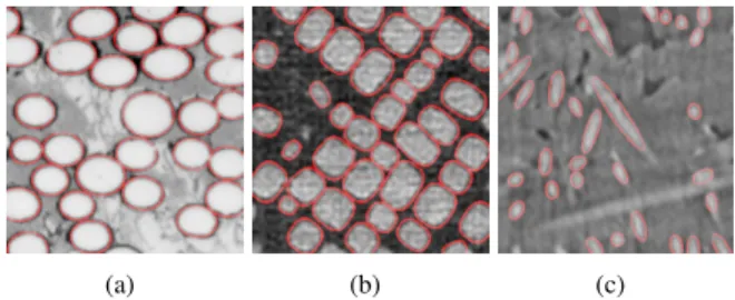
Previously proposed MPP shape models work well when the objects have similar size and shape in images, such as those shown in Figure1(a) and Figure1(b) which use el-lipses and super elel-lipses. However, these may not work well with fibers whose size vary over a wide range, as shown in Figure1(c), which miss the longest fiber. The approach is therefore both time-consuming and inaccurate in detection of fibers. There are mainly two reasons for the poor perfor-mance of MPP in this application. First, the long fiber can not be described by ellipse accurately. Second, the large variation

(a) (b) (c)

Fig. 1:(a) MPP result on ellipse fiber detection ; (b) MPP result on super ellipse fiber detection; (c) MPP result on long fiber detection.

of the fiber’s size increases the searching time.

In order to solve the problem of detecting long fibers in Figure1(c), we propose a connected-tube model based on a Marked Point Process. In our approach, instead of model-ing the long fiber by an ellipse object, we model it as a se-ries of connected tubes. Since the long fibers are modeled by connected tubes, the size of the tubes can be controlled in a smaller range.

The tube model can be combined easily with the ellipse or rectangle model to form a mixed MPP model. Compared with Lafarge et al. [10]’s approach, we replace the segments and lines by tubes, which have similar parameters and energy term as the ellipses, and the switching between tube and ellipse is simpler.

Moreover, we show that the connected-tube model can also be applied to road detection in 2D remotely sensed im-ages, which has been a popular topic in recent years [11–14]. When combined with a rectangle model, it is possible to de-tect the buildings and roads at the same time. Compared with the previously proposed Quality Candy model [15], our tube model has a much simpler prior for connection.

The paper is organized as follows: In Section 2, we de-scribe the proposed tube model under a mixed MPP frame-work. In Section 3, the optimization method is presented. In Section 4, experimental results for fiber detection in micro-scopic image, road and building detection in remotely sensed images are given. Conclusions are outlined in Section 5.

(3)

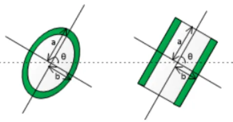
Fig. 2:Ellipse and Tube models

2 A Mixed Marked Point Process of

Ellipses and Tubes

The framework of the Mixed Marked Point Process of ellipses and tubes is similar to the framework of general multimarked point process in [10]. The point space is defined on an image lattice S = [0, Xmax] × [0, Ymax], S ⊂ IR2. The mark space

M is defined as the union of the ellipse mark set Meand the

tube mark set Mt, so M = Me ∪ Mt. In our model, an

ellipse object and a tube object have similar random variables for each mark, which makes it easier to switch between them, compared to the switch between an ellipse and a segment in [10]. Their shapes can be seen in Figure 2, where a,b are the major and minor axes which control the size of the ellipse and the tube respectively, and θ controls the orientation. Here, Me= Mt= [amin, amax] × [bmin, bmax] × [0, π], for some

parameters amin, amax, bmin, bmax.

A random marked object field W is a subset of S × M . A marked object is defined as a vector Wi= (Si, Mi) ∈ W . Let

ΩW be the configuration space, which denotes the space of

all possible realizations of W . Then w = (w1, ..., wn) ∈ ΩW

is a possible object configuration, where n is the number of objects in this configuration. Note the number of objects in the random field W is a random variable and could be quite a large number. Let Y be the observed image. Then the density of the mixture marked point process is given by

f (w|y) = 1

Zexp{−Vd(y|w) − Vp(w)} (1) where Z is the normalizing constant, Vd(y|w) is the data

en-ergy, which describes how well the objects fit the observed image, Vp(w) is the prior energy introducing the prior

knowl-edge on the object configuration.

2.1 Data Energy

Data energy Vd(y|w) is the sum of the individual object

ener-gies:

Vd(y|w) =

X

i

Vd(y|wi) (2)

where Vd(y|wi) describes how well object wifit the observed

image y. We associate an inner region Dinand outer region

Doutwith each object, shown as the white area and green area

inside objects in Figure 2, respectively. The outer area is set to be 2 pixels wide, good compromise for all the images tested. By defining the Bhattacharya distance B(y|wi) between the

inner region and outer region of each object, Vd(y|wi) can be

2.2 Prior Energy

Vp(w) describes the prior knowledge about objects. It is given

as Vp(w) = αVpol(w) + βV len p (w) + γV con p (w) (4) where Vol

p (w) penalizes overlapping between objects, Vplen(w)

penalizes the tubes with short length (the axis a); Vcon p (w)

encourages connections between tubes; and α, β and γ are weights for each term, which are set by trial and error. 2.2.1 Overlap Prior

The overlap prior Vpol(w) is applied to all objects.

Vpol(w) = X i,j Vpol(wi, wj) (5) V_pol(wi, wj) = ( R(wi, wj) if R(wi, wj) < Tol ∞ else (6)

where R(wi, wj) is the mutual overlap ratio between object

wiand wj as in [3]. Tolis the overlap threshold. It is set to

0.25 in our experiments. 2.2.2 Length Prior

Shorter tubes may over fit the observed image Y , which could unreasonably increase the dimension of object configuration w. So we introduce Vlen

p (w) to penalize the short tube

ob-jects. We let

V_plen(w) = X

wi∈wT

V_plen(wi) (7)

where wT is the collection of tube objects in w, Vplen(wi) =

exp((amax− ai)/amax), and ai is the major axis a of tube

object wi.

2.2.3 Connection Prior

To encourage the tubes to be connected, we introduce the con-nect prior Vpcon(w).

Vpcon(w) =

X

wi∈wT

(4)

(a) (b)

Fig. 3: (a) Joint area of a tube; (b) Illustration of connection rela-tionship between tubes.

(a) (b) (c)

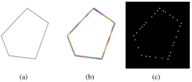
Fig. 4:(a) Polygon image; (b) Tubes detection result; (c) The con-nection map.

We define the front and back joint area at the two ends of a tube, as in Figure 3(a), where the blue part is the front joint area and the red part is the back joint area. Unlike the prior model used in the Quality Candy Model [15], we have no free, single or double connection relationship for tubes. Also we do not have orientation potential term for the alignment of tubes. From Figure 3(b), if the angle of two connected tubes is large, the overlapped area would be also large, which will penalize the orientation difference between two connected tubes.

In order to calculate the connection prior, we adopt a con-nection map, which has the same size as the observed image, to record the joint area of tubes in an object configuration. The map is initialized with zeros. When a tube is generated, the positions that correspond to the joint area of the tubes are incremented by one. Figure 4 shows an example of a connec-tion map.

With the connection map, the connection prior for each tube object Vpcon(wi) can be calculated as

V_pcon(wi) = 0.5 × Fcon(wi) + 0.5 × Bcon(wi) (9)

where Fcon(wi) =    1 −Rf(wi) Tcon if Rf(wi) < Tcon − √ Rf(wi)− √ Tcon 1−√Tcon else (10) Bcon(wi) =    1 −Rb(wi) Tcon if Rb(wi) < Tcon − √ Rb(wi)− √ Tcon 1−√Tcon else (11)

Rf(wi) is the connecting overlap ratio of a tube’s front joint

region in the connection map. Rb(wi) is the connecting

over-lap ratio of the tube’s back joint region on connection map. Tconis the connection threshold, which is set to 0.15 in our

experiments. These equations are used for penalizing connec-tions under Tcon, and encouraging a high connection rate.

3 Optimization Method

The conventional RJ MCMC algorithm [17] is used for find-ing the optimal configuration that minimizes the energy func-tion V (w|y) = Vd(w|y)+Vp(w). State transitions in the

con-figuration space are realized by three types of kernel: Birth and death kernel, perturbation kernel and switch kernel.

Birth and death kernel This kernel allows a dimension change in a configuration by adding or removing an object from w [9]. There are two types of objects in our configura-tion space. Tubes and ellipses are given the same probability for birth.

Perturbation kernel This kernel changes the marks ai, bi, θi

for each object wi in w. We choose Gaussion distributions

for updating the marks [17].

Switch kernel This kernel allows transition between tube objects and ellipse objects. Since we use the same marks for tubes and ellipses, the switch is simple. From tube object wt = (xt, yt, at, bt, θt) to an ellipse object we =

(xe, ye, ae, be, θe), we simply let xe= xt, ye= yt, be= bt,

θe= θt, ae = at+ X, where X ∼ N (0, 4). A switch from

an ellipse object weto a tube object wtis made in the same

way. In order to speed up the convergence, it is possible to use a Multiple Birth and Death algorithm [16, 18] instead of the classical RJMCMC [17]. This is what we did in the experiments.

4 Experiments

We apply the mixed MPP model to a series of fiber-reinforced composite materials images provided by industry. A compar-ison between our model and an ellipse-only MPP model is given. Also we test on some cut remotely sensed images from dataset [19] to show its potential to detect road network and buildings.

4.1 Fiber Detection

In the fiber detection tests, the parameters of our model are set as T = 50, Tol= 0.25, Tcon= 0.15, amin= 4, amax= 22,

bmin = 2, bmax = 8, α = 0.5, β = 0.12, γ = 0.38. These

(5)

(a) (b)

(c) (d)

Fig. 5: (a)Fiber-Reinforced Composite Materials image (Courtesy of Prof. Mike Sangid, Purdue University); (b) Hand drawn fibers (c) Ellipse-only MPP model result; (d) Mixed MPP model result.

results and are kept constant for all material images. Figure 3 presents the results of fiber detection in a microscopy image with dimension 308 × 308. From Figure 5(a), the ellipse-only MPP model, with long axis ranging from 2 to 70 pixels misses almost all long fibers , while our model can extract the long fibers. We use 10 images with dimension 308 × 308 to verify the performance of our model. The missed long fiber (with amax ≥ 18) rate, missed short fiber (with amax < 18) rate,

and over detection rate are listed Table 1. Our model not only outperforms the ellipse-only model for the long fiber detec-tion but also has lower missed detecdetec-tion rate. We believe this is because some short fibers can not be modeled as ellipses accurately. Unfortunately, this will also lead to higher false detection rate since fibers are modeled by two kinds of shape.

Missed detection rate for long fibers Missed detection rate for short fibers False detection rate ellipse MPP 81.53% 4.22% 2.10% mixed MPP 9.23% 1.40% 4.89%

Table 1: Fiber Detection Evaluation

4.2 Road Detection

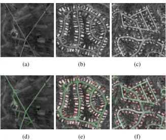
In the road detection problem, we test the proposed model on remotely sensed images to show the potential of it. Figure 6(a), (b), and (c) show three satellite images of road networks, trees, and buildings. Figure 6(d) shows the detection result by connected-tube model. In Figure 6(e), (f), we applied the mixed MPP model by replacing the ellipse model with a

rect-(a) (b) (c)

(d) (e) (f)

Fig. 6:Road detection. The upper row, original satellite images; the bottom row: our test result.

angle model for detecting buildings.

5 Conclusion

For extracting long strip features in images, we have proposed a connected-tube model based on marked point processes. In order to make the tubes connected well, a length prior and a connection prior are introduced. For fiber detection the tube model works well, when combined with the ellipse model in a mixed MPP framework. The tube model aims at detecting long fibers, while the ellipse model can detect short fibers. Since we use the same parameters to control the size and ori-entation of tubes and ellipses, switching between them is con-venient. This mixed model solves the problem of wide mark range in MPP model for detecting the fibers in microscopy image, and improves the accuracy of detecting. We present the result on fiber-reinforced composite materials images to show the advantages of our model. Furthermore the tests of our model on remotely sensed images shows its potential of detecting roads and buildings. More tests will be made in near future.

6 Acknowledgment

This research is supported by the Air Force Office of Sci-entific Research, MURI contract # FA9550-12-1-0458 and by the National Science Foundation(NSF) grant NSF CMMI MoM 16-62554.

J. Zerubia would like to thank the IEEE Signal Processing Society for financial support as IEEE SPS Distinguished Lec-turer in 2016-2017 which gave her the opportunity to meet with Prof. M. Comer and start this collaboration.

(6)

7 References

[1] J. P. Simmons, B. Bartha, M. D. Graef, and M. Comer, “Development of bayesian segmentation techniques for automated segmentation of titanium alloy images,” Mi-croscopy and Microanalysis, vol. 14(S2), pp. 602–603, 2008.

[2] J. P. Simmons, P. Chuang, M. Comer, J. E. Spowart, M. D. Uchic, and M De Graef, “Application and fur-ther development of advanced image processing algo-rithms for automated analysis of serial section image data,” Modelling and Simulation in Materials Science and Engineering, vol. 17, no. 2, pp. 025002, 2009. [3] H. Zhao, M. L. Comer, and M. De Graef, “A

uni-fied markov random field/marked point process image model and its application to computational materials,” pp. 6101–6105, 2014.

[4] J. Wang and B. Sharma M. D. Sangid F. Costa X. Jin C. L. Tucker III L. S. Fifield B. N. Nguyen, R. Mathur, “Fiber orientation in injection molded long carbon fiber thermoplastic composites,” in Proceedings of the Tech-nical Conference & Exhibition, 2015.

[5] R. F. Agyei, B. Sharma, and M. D. Sangid, “Inves-tigating sub-surface microstructure in fiber reinforced polymer composites via x-ray tomography characteriza-tion,” in 57th AIAA/ASCE/AHS/ASC Structures, Struc-tural Dynamics, and Materials Conference, 2016. [6] A. J. Baddeley and M. N. M. Van Lieshout, “Stochastic

geometry models in high-level vision,” Journal of Ap-plied Statistics, vol. 20, Issue 5-6, pp. 231–256, 1993. [7] X. Descombes and J. Zerubia, “Marked point process

in image analysis,” IEEE Signal Processing Magazine, vol. 19, Issue 5, pp. 77–84, 2002.

[8] J. Illian, A. Penttinen, H. Stoyan, and D. Stoyan, Statis-tical Analysis and Modelling of Spatial Point Patterns, Wiley-Interscience, 2008.

[9] C. J. Geyer and J. Møller, “Simulation and likehood in-ference for spatial point processes,” Scandinavian Jour-nal of Statistics, vol. 21, no. 4, pp. 359–373, 1994. [10] F. Lafarge, G. Gimel farb, and X. Descombes,

“Geomet-ric feature extraction by a multimarked point process,” IEEE Transactions on Pattern Analysis and Machine In-telligence, vol. 32, Issue 9, pp. 1597–1609, 2010. [11] J. D. Wegner, J. Montoya, and K. Schindler, “Road

net-works as collections of minimum cost paths,” ISPRS Journal of Photogrammetry and Remote Sensing, vol. 108, pp. 128–137, 2015.

[12] S. G. Jeong, Y. Tarabalka, N. Nisse, and J. Zeru-bia, “Progressive Tree-like Curvilinear Structure Recon-struction with Structured Ranking Learning and Graph Algorithm,” hhal − 01414864i, 2016.

[13] A. Schmidt, F. Lafarge, C. Brenner, F. Rottensteiner, and C. Heipke, “Forest point processes for the automatic extraction of networks in raster data,” ISPRS Journal of Photogrammetry and Remote Sensing, vol. 126, pp. 38–55, 2017.

[14] G. Moser and J. Zerubia (Ed.), Mathematical Models for Remote Sensing Image Processing, Springer Inter-national Publishing, 2018.

[15] C. Lacoste, X. Descombes, and J. Zerubia, “Point pro-cesses for unsupervised line network extraction in re-mote sensing,” IEEE Transactions on Pattern Analysis and Machine Intelligence, vol. 27, Issue 10, pp. 1568– 1579, 2005.

[16] X. Descombes, R. Minlos, and E. Zhizhina, “Object extraction using a stochastic birth-and-death dynamics in continuum,” Journal of Mathematical Imaging and Vision, vol. 33, Issue 3, pp. 347–359, 2009.

[17] P. J. Green, “Reversible jump markov chain monte carlo computation and bayesian model determination,” Biometrika, vol. 82, Issue 4, pp. 711–732, 1995. [18] Xavier Descombes, “Multiple objects detection in

bi-ological images using a marked point process frame-work,” Methods, vol. 115, pp. 2–8, 2017.

[19] V. Mnih, Machine Learning for Aerial Image Labeling, Ph.D. thesis, University of Toronto, 2013.