UNIVERSITÉ DU QUÉBEC À MONTRÉAL
LES IMPACTS BIOPHYSIQUES DES CHANGEMENTS DE L'UTILISATION DES TERRES EN AMÉRIQUE DU NORD AVEC LE MODÈLE RÉGIONAL DU
CLIMAT CANADIEN
MÉMOIRE PRÉSENTÉ
COMME EXIGENCE PARTIELLE
DE LA MAÎTRISE EN SCIENCES DE L'ATMOSPHÈRE
PAR
ARLETTE CONST ANZA CHA CON OELCKERS
Avertissement
La diffusion de ce mémoire se fait dans le respect des droits de son auteur, qui a signé le formulaire Autorisation de reproduire et de diffuser un travail de recherche de cycles supérieurs (SDU-522 - Rév.0?-2011). Cette autorisation stipule que ••conformément à l'article 11 du Règlement no 8 des études de cycles supérieurs, [l'auteur] concède à l'Université du Québec à Montréal une licence non exclusive d'utilisation et de publication de la totalité ou d'une partie importante de [son] travail de recherche pour des fins pédagogiques et non commerciales. Plus précisément, [l'auteur] autorise l'Université du Québec à Montréal à reproduire, diffuser, prêter, distribuer ou vendre des copies de [son] travail de recherche à des fins non commerciales sur quelque support que ce soit, y compris l'Internet. Cette licence et cette autorisation n'entraînent pas une renonciation de [la] part [de l'auteur] à [ses] droits moraux ni à [ses] droits de propriété intellectuelle. Sauf entente contraire, [l'auteur] conserve la liberté de diffuser et de commercialiser ou non ce travail dont [il] possède un exemplaire.>>
REMERCIEMENTS
Je tiens à remercier ma directrice de recherche Laxrni Sushama et mon co-superviseur Hugo Beltrami pour leur soutien.
Pour leur soutien inconditionnel, je tiens à remercier ma famille qui ont représenté un pilier fondamental à mon développement mental et professionneL
Je remercie aussi Melissa Cholette, Dominic Matte, Marilys Clement, Carolyne Pickler et Gregory Yang pour leur aide dans la traduction des séminaires et du mémoire. Je voudrais également remercier tous mes camarades de la promotion 2012, sans eux je aurrais pas surmonter la barrière linguistique.
Je tiens à remercier à Katja Winger et Luis Duarte pour lem assistance technique en ce qui concerne les simulations MRCC. Oleksandr Huziy et Camille Garnaud pour leur aide dans le traitement des ensembles de données et Gulilat Tefera Diro pour son soutien et ses commentaires.
Cette recherche a été financée par Conseil de recherches en sciences natmelles et en génie du Canada de subventions à la découverte (CRSNG-SD) et le programme chaires de recherche du Canada. J'ai bénéficié d'une boure d'etudes supérieyres à travers «CREA TE - Training Program in Climate Sciences » bourse d'études supérieures et Le Centre pour l'Étude et la Simulation du Climat à l'Échelle Régional (ESCER). Les ressources informatiques ont été fournies par l'Université du Québec à Montréal (UQAM) et Calcul Québec, un regroupement d'universités québécoises pour le calcul informatique de pointe (CIP).
LISTE DES FIGURES ... iv
LISTE DES ABRÉVIATIONS, SIGLES ET ACRONYMES ... vi
LISTE DES SYMBOLES ... ix
RÉSUMÉ ... x
CHAPITRE! INTRODUCTION ... 1
CHAPITRE II LES IMPACTS BIOPHYSIQUES DES CHANGEMENTS DE L'UTILISATION DES TERRES EN AMÉRIQUE DU NORD AVEC LE MODÈLE RÉGIONAL DU CLIMAT CANADIEN ... 7
BIOPHYSICAL IMPACTS OF LAND USE CHANGE OVER NORTH AMERICA AS SIMULA TED BY THE CANADIAN REGIONAL CUMA TE MO DEL ... 8
ABSTRACT ... 9
2.1 Introduction ... 10
2.2 Model and Methods ... 13
2.2.1 The Canadian Regional Climate Model.. ... 13
2.2.2 Methodology ... 14
2.3 Results ... 17
2.3 .1 Spatial Seasonal Analysis ... 17
2.3 .2 Anal y sis of Average Annual Cycles ... 19
CHAPITRE III CONCLUSION ... 25
APPENDICE A FIGURES ... 28
APPENDICES SUPPLEMENTARY MATERIAL ... 38
LISTE DES FIGURES
Figure Page
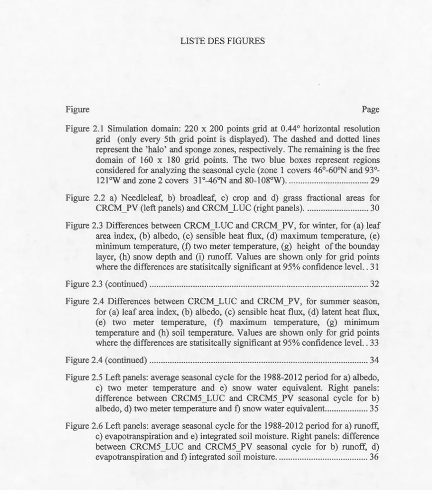
Figure 2.1 Simulation domain: 220 x 200 points grid at 0.44 ° horizontal resolution grid ( only every 5th grid point is displayed). The dashed and dotted lines represent the 'halo' and sponge zones, respectively. The remaining is the free domain of 160 x 180 grid points. The two blue boxes represent regions considered for analyzing the seasonal cycle (zone 1 covers 46°-60°N and
93°-1210W and zone 2 covers 31°-46°N and 80-108°W) ... 29 Figure 2.2 a) Needleleaf, b) broadleaf, c) crop and d) grass fractional areas for CRCM_PV (left panels) and CRCM_LUC (right panels) ... 30 Figure 2.3 Differences between CRCM_LUC and CRCM_PV, for winter, for (a) leaf
area index, (b) albedo, (c) sensible heat flux, (d) maximum temperature, (e) minimwn temperature, (f) two meter temperature, (g) height of the bounday layer, (h) snow depth and (i) runoff. Values are shown only for grid points where the differences are statisitcally significant at 95% confidence level. . 31 Figure 2.3 ( continued) ... 32 Figure 2.4 Differences between CRCM_LUC and CRCM_PV, for summer season, for (a) leaf area index, (b) albedo, ( c) sensible heat flux, ( d) latent heat flux, ( e) two meter temperature, (f) maximwn temperature, (g) minimum temperature and (h) soil temperature. Values are shown onJy for grid points where the differences are statisitcally significant at 95% confidence level.. 33 Figure 2.4 (continued) ... 34 Figure 2.5 Left panels: average seasonaJ cycle for the 1988-2012 period for a) albedo, c) two meter temperature and e) snow water equivalent. Right panels: difference between CRCM5_LUC and CRCM5_PV seasonal cycle for b) albedo, d) two meter temperature and f) snow water equivalent... ... 35 Figure 2.6 Left panels: average seasonal cycle for the 1988-2012 period for a) runoff,
c) evapotranspiration and e) integrated soil moisture. Right panels: difference between CRCM5_LUC and CRCM5_PV seasonal cycle for b) runoff, d) evapotranspiration and f) integrated soil moisture ... 36
Figure 2.7 Left panel: average seasonal cycle for the 1988-2012 period for a) precipitation. Right panel: difference between CRCM5_LUC and CRCM5
YV
seasonal cycle for b) precipitation ... 37ARC BU-MODIS CIP CLASS COz CRCM5 - - - -- - - - -
-LISTE DES ABRÉVIATIONS, SIGLES ET ACRONYMES
Advanced Research Computing
Boston University's Moderate Resolution Imaging Spectrometer (US)
Méthane
Methane
Calcul Informatique de Pointe
Canadian Land Surface Scheme, version 3.5 (Canada)
Dioxyde de Carbone
Carbon dioxide
Canadian Regional Climate Mode!, version 5 (UQAM, Canada)
CRCM5 LUC CRCM5 simulation using potential vegetation dataset
CRCM5 PV CRCM5 simulation using the vegetation that has presence ofLUC
CREA TE Training Program in Climate Sciences
ECMWF European Centre Medium-Range Weather Forecasts (Europe)
ERA-40 Second generation reanalysis ofECMWF
ESCER Centre pour 1 'Étude et la Simulation du Climat à 1 'Échelle Régional
GCM Global Climate Model
GEM Global Environmental Multiscale model developed by the Canadian Meteorological Centre (CMC, Canada)
LAI Leaf Area Index
LHF Latent Heat Flux
LUC Land Use Change
MCG Modèle climatique global
MRCCS Modèle régional canadien du climat, cinquième version (UQAM, Canada)
N North
NSERC-DG Natural Sciences and Engineering Research Council of Canada Discovery Grant
NWP Numerical Weather Prediction
SHF Sensible Heat Flux
SPOT Satellite Pom l'Observation de la Terre
T2M Two meter temperatme
TMax Maximum Temperature
UQAM
us
w
Université du Québec à Montréal
United States
West
cm km m mm/day mm/month W/m2 0 % Centimeter
Kilogram per meter square Kilometer
Kilomètre carré Kilometer square Meter
Millimeter per day Millimeter per month Watt per square me ter Degrees Celsius
Degrees of latitude and longuitude
Pourcentage Percentage
RÉSUMÉ
Les changements dans 1 'utilisation des terres sont des manifestations évidentes de l'activité humaine de par le changement de la végétation naturelle par des terres cultivées. Cela modifie les caractéristiques biophysiques de la région et affecte le climat local. Ce projet a pour but d'étudier les impacts des effets biophysiques des changements dans l'utilisation des terres sur le climat régional en Amérique du Nord.
La cinquième génération du Modèle Régional Canadien du Climat (MRCC5) a été utilisé afin de comparer deux simulations utilisant différents ensembles de données de la couverture terrestre. Le premier ensemble de données représente la végétation terrestre sans activité humaine de par l'absence de terres cultivées (végétation potentielle) et le deuxième ensemble est l'utilisation actuelle des terres correspondant à la fusion de la végétation potentielle et de ten·es cultivées. Dans la simulation utilisant le deuxième ensemble de données, les forêts et les prairies sont remplacées par des tenes cultivées dans les régions centre-ouest des Etats-Unis et centre-sud du Canada. Par conséquent, les caractéristiques de surface, comme la couvetture fractionnaire de végétation, 1 'indice de surface foliaire, 1 'albédo, la longueur de rugosité et la profondeur des racines, sont différentes de la simulation utilisant le premier ensemble de données. Les deux simulations couvrent la période de 1988-2012 et les conditions aux frontières latérales sont fournies par les réanalyses ERA-Interim. La couverture de glace et la température de surface de la mer sont également données par ERA-Interim.
La comparaison des deux simulations suggère des valeurs d'albédo plus élevées en hiver sur les régions où il y a des changements dans 1 'utilisation des terres. L'absence de cultures en hiver conduit à une rétroaction positive avec la neige. Ces valeurs plus élevées d'albédo se reflètent dans des valeurs plus basses de la température à 2 mètres. Certaines régions, comme l'est d~s Etats-Unis, montrent également un refroidissement en été pour la simulation avec changements dans l'utilisation des tenes en raison de flux de chaleur latente plus élevés et de flux de chaleur sensible plus basse. Les cycles annuels de certaines variables d'intérêts ont été analysés pour deux régions où les changements dans 1 'utilisation des tetTes sont manifestes, à savoir le centre-sud du Canada et le centre-nord des États-Unis. L'analyse des cycles saisonniers suggère que l'effet de refroidissement dû aux changements dans 1 'utilisation des terres est présent durant toute l'année. Les impacts des changements dans 1 'utilisation des terres sur l'évapotranspiration, l'humidité du sol et les précipitations sont également présents tout au long du cycle annuel. Cependant, les
impacts des changements dans l'utilisation des terres sur les eaux de ruissellement se limitent essentiellement à la saison de la fonte des neiges.
Cette étude a permis de fournir des informations utiles concernant les impacts des changements dans l'utilisation des terres sur le climat et l'hydrologie de l'Amérique du Nord.
Mots clés: impacts biophysiques, changements dans 1 'utilisation des terres, modélisation régionale du climat, Amérique du Nord
CHAPITRE I
INTRODUCTION
À travers le temps, le climat et l'environnement de notre planète ont été fortement modifiés par les activités humaines [Mahmood et al., 201 0]. Ces modifications se reflètent entre autres. Dans l'évolution des ressources en eau, dans les émissions de gaz traces dans 1 'atmosphère et dans les changements de l'utilisation des tenes [GIEC, 2014]. Ce dernier est la manifestation la plus évidente des activités humaines, par la déforestation et par la transformation des prairies naturelles en des zones urbaines ou des teiTes cultivées [DeFries et al., 2004; CEC, 2008]. Par exemple, en date de l'année 2000, une superficie globale de 15 millions de km2 de savanes, prairies et forêts, a été remplacée par des cultures à des fins agricoles. Cette superficie représente presque 40% de la surface libre de glace de la Tene [Foley et al., 2005]). Les régions les plus touchées étaient le sud de l'Asie, le sud de l'Europe et les États-Unis [Ramankutty et al., 2008; Klein et al., 2011].
Le climat peut être influencé par les changements dans 1 'utilisation des tenes via des interactions biogéochimiques et biophysiques. Les effets biogéochimiques modifient la composition des gaz atmosphériques en augmentant la concentration des gaz à effet de serre, comme le C02 et CH4, ce qui provoque une rétroaction positive de réchauffement [Georgescu et al., 2010; Boysen et al, 2014.; Friedlingstein et al., 2004]. Les effets biophysiques influent sur le budget de l'énergie de surface en modifiant les flux de chaleur sensible, les flux de chaleur latente et le budget de l'eau de surface en altérant la répartition des précipitations dans l'évapotranspiration, Je
ruissellement et la teneur en eau du sol [Bonan, 2008; Davin et al., 2010; de Norblet-Ducourdré et al., 2012]. Ces modifications sont une conséquence des changements dans les caractéristiques de surface résultant du remplacement des forêts par des
terres cultivées ou des prairies. Par exemple, l'albédo, qui joue un rôle important dans
le budget du rayonnement net de la Terre, est plus faible pour les forêts que pour les pâturages ou les terres cultivées. La profondeur des racines, qui détermine la quantité d'eau disponible pour la transpiration, est plus grande pour les arbres comparativement aux cultures, ce qui permet d'extraire davantage d'eau des couches profondes, conduisant donc à des valeurs plus élevées d'évapotranspiration [Bonan,
2008; Pitman et al., 2011; Mahmood et al., 2014].
Pour comprendre l'influence des changements dans 1 'utili ation des terres, les modèles numériques du climat sont généralement employés [Brovkin et al., 2006]
afin de comparer des simulations sans changements dans l'utilisation des terres avec
des simulations ayant des changements dans l'utilisation des terres. En utilisant cette
méthodologie, des études antérieures ont montré que les changements dans
l'utilisation des terres provoquent un refroidissement à l'échelle globale [Brovkin et al., 1999; Feddema et al., 2005; Brovkin et al., 2006], mais qu'il y a beaucoup de disparités au niveau régional. Plus précisément, les modèles ont montré un refroidissement dans les hautes latitudes et les latitudes tempérées latitudes de l'Amérique du Nord, et un réchauffement dans les latitudes tropicales [Laurent et Chase, 2010; Bonan et al., 1997]. Le refroidissement des hautes latitudes peut être
directement et/ou indirectement attribué à l'augmentation de l'albédo, à la réduction de longueur de rugosité et à la diminution de l'indice de surface foliaire en raison du
changement des forêts par des cultures [Bonan, 2008; Findell et al., 2007; Pitman et
al., 2011]. D'autre part, le réchauffement des latitudes tropicales peut être dû à la diminution de l'évapotranspiration et à l'augmentation du :flux de chaleur sensible,
principalement en raison de la diminution de la profondeur d'enracinement [Pielke,
3
Toutefois, il y a encore des incertitudes sur la façon dont les changements dans l'utilisation des terres modifient le climat en raison des questions concernant
l'exactitude des les ensembles de données de végétation [Oelson et al., 2004] et sur
les caractéristiques des modèles climatiques [Findell et al., 2007]. Par exemple, Hua et Chen (2013) a montré que les changements dans l'utilisation des terres affectent le
cycle diurne de température dans les régions des latitudes moyennes de l'Amérique du Nord, de l'Amérique du Sud et de l'Eurasie, et ce, pour la période de 1971 à 2000. Le cycle diurne est effectivement affecté par une augmentation du flux de chaleur latente
et une plus grande couverture nuageuse, ce qui entraîne une diminution des
températures maximales quotidiennes. Cette étude a également révélé une
augmentation de la température minimale quotidienne en Inde, ce qui a entraîné des
changements dans l'albédo et l'évapotranspiration. Pitman et al., (2009) ont étudié les impacts des changements dans l'utilisation des terres en utilisant six modèles climatiques globaux (MCG). Leurs résultats suggèrent une diminution statistiquement
significative du flux de chaleur latente dans la moitié des MCG, tandis que l'autre
moitié montre une augmentation du flux de chaleur latente dans l'hémisphère nord au cours de l'été. D'un autre côté, cinq des six simulations suggèrent une diminution de la température de surface. Ces différences entre les MCG peuvent être attribuées
principalement aux différences dans: (a) la configuration des changements dans 1 'utilisation des terres dans les modèles de végétation de surface, (b) la représentation
de la phénologie des cultures, (c) le paramétrage de l'albédo et (d) la représentation de l'évapotranspiration pour différents types d'occupation du sol. Les expériences de
modèles climatiques globaux discutés ci-dessus suggèrent que les impacts des
changements dans 1 'utilisation des terres devraient être davantage étudiés de manière régionale [Fedeman et al., 2005; Findell et al., 2007; Pitman et al., 2009; Pielke et
al., 2011].
C'est pourquoi des études à l'échelle régionale ont été effectuées afin de mieux
et al. (2007), étude d'impacts des changements dans l'utilisation des terres sur la région de la Chine, ont constaté que les changements dans 1 'utilisation des terres permettent (1) le renforcement de la circulation de la mousson, (2) la diminution des précipitations sur les régions méridionales de la Chine, (3) 1 'augmentation des précipitations sur le nord de la Chine en hiver et (4) un effet de refroidissement de la température moyenne annuelle. Des études sur les régions tropicales ont montré une diminution de l'évapotranspiration, résultant principalement de la diminution de la profondeur des racines en raison des changements dans l'utilisation des terres,
conduisant à une augmentation de la température et à une diminution des
précipitations [Nogherotto et al., 2013 ; Akkermans et al., 2014.; Lawrence & Vandecar, 2015].
Au cours des dernières années, l'Amérique du Nord a été une région fortement influencée par des changements dans l'utilisation des terres. Son impact a été détecté dans des études antérieures avec des MCG, mais pour une meilleure compréhension de cette influence, il est utile de réaliser des études à l'échelle régionale. Pour cette raison, cette étude se concentre sur les effets biophysique du changement dans l'utilisation des terres en Amérique du Nord avec une résolution plus élevée, en utilisant la cinquième génération du modèle régional canadien du climat (MRCCS)
couplé avec le schéma canadien de paramétrisation de la surface terrestre (CLASS).
L'objectif de cette étude est d'évaluer les impacts des changements dans 1 'utilisation
des terres sur le climat en Amérique du Nord en utilisant des expériences
soigneusement conçues avec la cinquième génération du modèle régional canadien du
climat (MRCCS). Seuls les impacts biophysiques des changements dans 1 'utilisation des terres seront considérés dans cette étude. Deux simulations utilisant différents ensembles de données de végétation seront produites: (1) avec une végétation potentiel, donc sans l'influence des activités humaines et (2) un ensemble de données qui correspond à l'utilisation actuelle des terres, représenté par l'ensemble de données de végétation potentielle intégré à un ensemble de données de terres cultivées. Les
5
deux expériences seront comparées entre elles afm d'évaluer les impacts des
changements dans l'utilisation des terres sur les caractéristiques de· surface et des différents flux.
Organisation du mémoire
Pour faire suite à cette introduction, un article rédigé en anglais correspond au chapitre II de ce mémoire. Cet article comprend l'Introduction (section 2.1) pour discuter du cadre théorique et l'objectif de l'étude. Puis, il y les descriptions du modèle et de la Méthodologie (section 2.2), suivi de la présentation des Résultats (section 2.3) qui se concentrent sur la comparaison entre simulations pour les saisons d'hiver et d'été, et sur l'évaluation de variables de surface et de cycles annuels. Finalement, la section 2.4 fournit le résumé et les conclusions de cet article. Les conclusions de ce mémoire seront présentées au chapitre III et le chapitre IV liste les références.
CHAPITRE II
LES IMPACTS BIOPHYSIQUES DES· CHANGEMENTS DE L'UTILISATION
DES TERRES EN AMÉRIQUE DU NORD AVEC LE MODÈLE RÉGIONAL DU CLIMAT CANADIEN
Ce chapitre, présenté sous fonne d'un article rédigé en anglais, est principalement concentré sur les impacts biophysiques des changements de l'utilisation des terres sur
l'Amérique du Nord avec la cinquième génération ·du Modèle Régional Canadien du
Climat (MRCC5). Ce chapitre contient les descriptions du MRCCS, des expériences,
BIOPHYSICAL IMPACTS OF LAND USE CHANGE OVER NORTH AMERICA AS SIMULATED BY THE CANADIAN REGIONAL CLIMATE MODEL
by
Arlette Chacôn',I, Laxmi Sushama1 and Hugo Beltrami2
1
Centre pour l 'Ètude et la Simulation du Climat à l'Échelle Régionale (ESCER), Département des Sciences de la Terre et de l'Atmosphère, Université de Québec à
Montréal, Montréal, Québec, Canada. 2
Climate & Atmospheric Sciences lnstitute (CASI) and Department of Earth Sciences,
St. Francis Xavier University, Antigonish, Nova Scotia, Canada.
Submitted at Atmosphere- Open Access Journal
Received: 4 November 20151 Accepted: 19 February 20161 Published: 26 February 2016
*Corresponding author's address: Arlette Chacôn
Centre ESCER, Départment des Sciences de la Terre et de 1 'Atmosphère, UQAM BP 8888, Suce. Centre-ville
Montréal (Québec) Canada, H2H 212 e-mail: achacon@sca.uqam.ca
9
Abstract
This study investigates the biophysical impacts of human-induced land use change
(LUC) on the regional climate ofNorth America, using the fifth generation Canadian
Regional Climate Mode! (CRCM5). To this end, two simulations are performed with
CRCMS using different land cover datasets, one corresponding to the potential
vegetation and the other corresponding to current land use, spanning the 1988-2012 period, driven by European Centre for Medium-Range Weather Re-Analysis (ERA)-Interim at the lateral boundaries. Compari on of the two suggests higher albedo values, and therefore cooler temperatures, over the LUC regions, in the simulation with LUC, in winter. This is due to the absence of crops in winter, and also possibly
due to a snow-mediated positive feedback. Sorne cooling is observed in surnmer for the simulation with LUC, mostly due to the higher latent beat fluxes and lower
sensible heat fluxes over eastern US. Precipitation changes for these regions are not
statistically significant. Analysis of the annual cycles for two LUC regions suggests that the impact of LUC on two meter temperature, evapotranspiration, soil moisture
and precipitation are present year rOtmd. However, the impact on runoff is mostly
restricted to the snowrnelt season. Thjs study thus highlights regions and variables
most affected by LUC over North America.
Keywords: biophysical impacts; land use change; regional climate modeling; North
2.1 Introduction
The climate and the general environment of our planet have been strongly modified by human activities [Mahmood et al., 2010] through time that are reflected in changes
in emissions of trace gases into the atmosphere and land use change (LUC) [IPCC,
2014]. However, the most obvious manifestation of human activities is seen in the
latter, in the form of deforestation or transformation of natural grasslands into urban
or cropland areas [DeFries et al., 2004; CEC, 2008]. As of year 2000, savannas,
grasslands and forests, with a global area of 15 million krn2 (which is almost 40% of
Earth's ice free land surface [Foley et al., 2005]), have been replaced for agricultural
pw-poses, with LUC being largest over south and southeast Asia, Europe and the
United States (US) [Ramankutty et al., 2008; Klein Goldewijk et al., 2011].
Climate can be influenced by LUC through biogeochemical and biophysical
interactions. The biogeochemical effects alter the atmospheric gas composition by modifying greenhouse gases, such as C02 and C&; this increase in the concentration
of greenhouse gases can further augment climate warming through a positive
feedback [Georgescu et al., 2010; Boysen et al., 2014; Friedlingstein et al., 2004]. The biophysical effects influence the surface energy budget by altering the sensible and latent heat fluxes and the surface water budget by alterating the partitioning of
precipitation into evapotranspiration, runoff and soi] water content [Bonan, 2005;
Davin et al., 2010; Norbley-Ducourdré et al., 2012]. These alterations are a
consequence of the changes in surface characteristics resulting from replacing forests
by croplands or grasslands. For example, forests have lower albedo than pastures or
croplands. Therefore, clearing forests or transfonning grasslands to croplands results
in higher albedo values. Another important variable is root depth, which determines transpiration. Trees with deeper roots compared to crops extract water from deeper layers, leading to higher evapotranspiration values [Bonan, 2008; Pitman et al., 2011;
11
To understand the influence of LUC, nurnerical climate models are generally employed [Brovkin et al., 2006]. Usually, two simulations, with and without LUC,
are perforrned with global or regional climate mode! to assess the impact of LUC. Using this methodology, past studies have shown that LUC causes a cooling at the global scale [Brovkin et al., 1999; Feddema et al., 2005; Brovkin et al., 2006],
though there are important differences regionally. LUC is shown to cool temperatures
in the high and temperate latitudes of North America, while warrning is noted for the tropical latitudes [Lawrence and Chase, 2009; Bonan et al., 1997]. This can be directly and/or indirectly attributed to increases in albedo, reduction in roughness length and leaf area index due to the change of forest to crops in high and temperate latitudes [Bonan, 2005; Findell et al., 2007; Pitman et al., 2011]. On the other hand,
the LUC associated wanning presented in the tropical latitudes is due to the reduction of evapotranspiration and an increase in sensible heat flux, primarily due to the decrease in rooting depth [Pielke, 2001; Fedeman et al., 2005].
Nevertheless, there is still uncertainty about how LUC alters the climate due to questions about the accuracy of the vegetation datasets [Oelson et al., 2004] and the characteristics of the climate models [Findell et al., 2007]. For example, Hua and Chen (2013), in their global scale study, for the period of 1971 to 2000, found that LUC affects the diurnal temperature range in the mid-latitude regions of North America, South America and Eurasia and increases the latent heat flux, enhancing the cloud cover, thus resulting in decreased daily maximum temperatures. This tudy also
found a decrease in the diurnal temperature range over India that was due to an increase in the daily minimum temperature, which resulted from changes in albedo and evapotranspiration. Pitman et al. (2009) studied the impact of LUC using six
global climate models (GCMs), and their results suggest statistically significant decreases in the latent heat flux in three GCMs and increa es in the other tlu·ee GCMs, for the northem hemisphere during summer. However, for the near-surface temperature five GCMs suggest cooling and the sixth one suggests wanning. These
differences between the GCMs can be attributed primarily to the differences in: (a) the implementation of LUC in the vegetation/land surface models, (b) representation of crop phenology, (c) parametrization of albedo and (d) representation of
evapotranspiration for different land cover types, among others. Despite these
differences, the above discussed GCM experiments suggest that the impacts of LUC are more regional in nature [Fedeman et al., 2005; Findell et al., 2007; Pitman et al., 2009; Pielke et al., 2011].
Taking this into consideration, studies at regional scale have been performed to further understand the impact of LUC. For example, Gao et al., (2007) in their study of the impacts of LUC over China found that LUC reinforces the monsoon circulation, reduces precipitation over the southem regions of China and increases precipitation over the north in winter (opposite situation happens during summer), and causes a cooling effect in the annual mean temperature. Regional studies over tropical regions, confirming global studies discussed above, have shown that a decrease in evapotranspiration, mainly resulting from the reduction in root depth due to LUC, lead to an increase in temperature and a reduction in precipitation
[Nogherotto et al., 2013; Akkermans et al., 2014; Lawrence & Vandecar 2015]. In the past years, North America has been a region greatly irrfluenced by LUC. Its impact was detected in past studies with GCMs, but for better understanding of this influence, it is useful to perform regional scale studies. For this reason, this study is
focused on the biophysical effects of LUC over North America in a higher resolution,
using the fifth generation Canadian Regional Climate model (CRCM5) coupled with the Canadian Land Surface Scheme (CLASS). Two simulations using different vegetation datasets are used: ( 1) a potential vegetation datas et without the influence of human activities and (2) a dataset that corresponds to current land use, represented by the potential vegetation dataset modified for land use using a cropland dataset. The aim of this study is to understand how climate has been altered by the change in
13
potential vegetation due to land use changes and how this change affects surface characteristics and fluxes for various seasons.
The paper is organized as follows. A brief description of the mode! and the methodology is presented in section 2.2. The impacts of land use change are presented in section 2.3, followed by summary and conclusions in section 2.4.
2.2 Mode! and Methods
2.2.1 The Canadian Regional Climate Mode!
The mode! used in this study is CRCM5 [Martynov et al., 20 12], which is based on a limited-area version of the Global Environment Multiscale (GEM) mode! used for Numerical Weather Prediction (NWP) at Environment Canada [Côté et al., 1998]. GEM employs semi-Lagrangian transport and (quasi) fully implicit stepping scheme. In its full y elastic non-hydrostatic formulation [Y eh et al., 2002], GEM uses a vertical coordinate based on hydrostatic pressure [Laprise, 1992]. The following GEM parameterisations are used in CRCM5: deep convection following Kain and Fritsch ( 1990), shallow convection based on a transient version of Kuo (1965) scheme [Bélair et al., 2005], large-scale condensation [Sundqvist et al., 1989], correlated-K solar and terrestrial radiations [Li and Barker, 2005], subgrid-scale orographie gravity-wave drag [McFarlane, 1987], low-level orographie blocking [Zadra et al., 2003], and turbulent kinetic energy closure in the planetary boundary layer and vertical diffusion [Benoit et al., 1989; Delage and Girard, 1992; Delage, 1997].
The land surface scheme in CRCM5 is the Canadian Land Sw-face Scheme [CLASS, Verseghy 1991, 2011; Verseghy et al., 1993]. CLASS is set up with 26 soi! layers reaching a depth of 60 m, instead of the default three layers with a total depth of 4.1 m, in this study. It includes prognostic equations for energy and water conservation, and a thermal and hydrologically distinct snowpack where applicable (treated as a variable-depth layer). The hydrological budget is calculated only for the layers above
the bedrock, but the energy balance and the thermal budget are calculated for the
whole soil depth. In an attempt to crudely mimic subgrid-scale variability, CLASS
adopts a pseudo-mosaic approach and divides each grid cell into a maximum of four sub-areas: bare soil, vegetation, snow over bare soi] and snow with vegetation. For
each sub-area the water and energy balance are calculated separately and then
averaged over the grid cell. Also, CLASS recognizes 4 main vegetation categories:
needleleaf trees, broadleaf trees, crops and grasses. For each type of vegetation, the structural attributes such as leaf area index, roughness length, canopy mass and
rooting depth have to be specified if they are present in a grid ce il.
2.2.2 Methodology
The aim ofthis study as discussed above is to assess the impact of LUC on the North
American climate. To this end, as mentioned earlier, two CRCM5 simulations, with
different land caver datasets, i.e. one with potential vegetation, or in other words
vegetation that would exist if the region was void of human activity, and the other
representing exclusively the present-day land use of cropland, are performed. These
simulations will be referred to as CRCM5_PV and CRCM5_LUC, hereafter.
The potential vegetation dataset used in CRCM5 _PV cornes from Ramankutty and
Foley (1999), which includes 15 vegetation types, available at 5 min resolution. This
dataset is mainly derived from the DISCover dataset [Loveland and Belward, 1997]
for the April 1992 to March 1993 period, where the potential vegetation for areas
subject to land use were modified using the dataset ofHaxeltine and Prentice (1996).
More details about this dataset can be found in Ramankutty and Foley (1999).
A new vegetation dataset obtained by merging the potential vegetation dataset from
CRCM5 _PV and the cropland dataset of Ramankutty et al. (2008) is used in
CRCM5_LUC. Ramankutty et al. (2008) compiled this cropland dataset such that it is
consistent with the Food and Agriculture Organization's (F AO) definition of' Arable
15
humans have had on LUC. This dataset is created by combining global agricultural inventories from 1998 to 2002 (the proxies for that period were used when data were unavailable) along with data from satellites from the Boston University's Moderate resolution Imaging Spectrometer (BU-MODIS) [Friedl et al., 2002] and the Satellite Pour l'Observation de la Terre (SPOT) VEGETATION [Bartholome and Belward, 2005]. The potential vegetation fractions were reduced for ceJis with LUC in CRCM5_LUC, such that the total fractional area is 1.
The CRCM5 simulations are perforrned over a grid covering North America and adjoining oceans (Figure 2.1), at 0.44° horizontal resolution (-50 km), for the 1979-2012 period. The soil moisture and temperature fields are initialized with values obtained by spinning CLASS offline for 100 years, driven by European Centre for Medium-Range Weather Forecasts Reanalysis (ERA)-40 reanalysis for the 1958-1978 period repeatedly, using respective vegetations in the two spin-up simulations. The CRCM5 simulation for the 1979-2012 period were driven at the lateral boundaries by ERA-Interim reanalysis data [Dee et al., 20 11] from the European Centre for Medium-Range Weather Forecasts (ECMWF) and the frrst 9 years are considered as spin-up and therefore not included in the analysis presented in the paper. The ERA-Interim data is available at 0.75° horizontal resolution (- 80 km). The fractioned areas of the 4 main categories of vegetation considered for CRCM5_PV and CRCM5_LUC simulations are shown in Figure 2.2.
In CRCM5 _LUC simulation, large parts of the grasslands over the central regions of the US and the Canadian prairies, are replaced with cropland. Small fractions of broadleaf and needleleaf are also replaced with crops, particularly in the north-east US and central Canada. The seasonal variations in the morphological characteristics of the 4 main vegetation categories are taken into account in CLA [Verseghy, 1991 and Verseghy et al., 1993]. During maturity and/or fully leafed periods, the growth index bas a value of 1, while it is 0 during leafless periods. The transition period
between these two states is assumed to be linear, lasting up to 2 months for needleleaf trees and up to 1 month for broadleaf trees. For the growth index of crops, Earth is divided in 10° latitudinal bands (in both hemispheres). The tart of growing season and the end of harvest are set to occur on certain days of the year based on average dates from the Food and Agriculture Organization of the United Nations (UN F AO)
for regions above 30°N. It is assumed that it takes 2 months for crops to reach maturity and 1 month between the beginning of senescence and the end of harvest.
For grass, the growth index is set at 1 all year round because the annual variation in height and leaf area index are negligible. The roughness Jength of trees does not undergo seasonal variation, therefore is always equal to the maximum value. The height of crops and grasses varies (Iower than the maximum height) because of partial burying by snow and, for crops, an immature growth stage. The rooting depth of trees and grasses remain at their maximwn values as they are not affected by snow cover. However, for crops, it is corrected for its growth stage. The leaf area index presents seasonal variations and ranges between its minimum and maximwn values. For trees,
this variable is unaffected by the presence of snow. As for crops and grasses, the presence of snow must be taken into account for its calculation. On the other hand, for trees, both visible and near-infrared albedo are set to their average observed values but under leafless conditions, different values are set for the case of snow -cover and that of snow-free grou nd un der the canopy. Wh en half of the leaves have fallen, albedo varies linearly with leaf area index. For crops and grass, the leaf area index does not go below 1; therefore, the albedo values remain and do not vary from fully leafed values except when the ground is snow-covered. CLASS simulates reasonably well the seasonal variations in the canopy parameters, when proper fractional vegetation cover is specified. Validation of the previous version of CLASS has been performed as part of Project for Inter-comparison of Land Surface Parameterization (PILPS) [Henderson- elier et al., 1995; Bender on- ellers et al., 1996; Pitman & Henderson-Sellers, 1998]. Langlois et al. (2014) and Haghnegahdar
17
et al. (2014), have evaluated the performance of the recent version 3.5 ofCLASS, but when coupled with RCMs, focusing on snow simulations and hydrological modelling. The biophysical effects of LUC over North America on selected surface variables and fluxes are assessed by comparing CRCM5_LUC and CRCM5_PV simulations. The statistical significance of these differences is assessed through a t-test at 95% confidence level.
2.3 Results
2.3.1 Spatial Seasonal Analysis
The differences between CRCM5 LUC and CRCM5 PV for the winter artd summer months are presented here. References are made to other seasons where required. Figure 2.3 shows the differences between CRCM5_LUC and CRCM5_PV for selected surface fluxes and variables for the winter season. Regions with statistically significant differences in leaf area index (LAI) show a dipole pattern, with smaller LAI values in the north and higher values in the south in CRCM5_LUC compared to CRCM5 _PV (Figure 2.3a). This is because, for the northerly regions, the growing season for crop is mostly limited to the spring--early fall periods, leading to zero LAI in winter in CRCM5_LUC. However, for the southem regions (below 30°N), growing season for crops is year round as for broadleaf trees and therefore the LAI values are higher in CRCM5_LUC compared to CRCM5_PV (Figure 2.3a). Note that for this southern region, fractional areas of both grass and broadleaf were replaced with crops. The above changes to LAI leads to statistically significant differences in albedo between CRCM5_LUC and CRCM5_PV over these LUC regions, particularly for the northem regions (Figure 2.3 b ), where albedo value are higher in CRCM5_LUC compared to CRCM5_pV. The regions south of 30°N show slightly higher values of albedo in CRCM5 _LUC, despite the higher values of LAI, which is due to relatively drier soil layer at the surface in this simulation. The higher values of
albedo in CRCM5_LUC are reflected in the negative differences in sensible beat flux
(SHF, Figure 2.3c) and two rneter temperatures (T2M). The differences in T2M is
more than 1.4 °C over central Canada and central east US (Figure 2.3d). The signature of high albedo in CRCM5_LUC can also be seen in the lower values of the daily minimum (TMin) and maximum (TMax) temperatures; the maximum differences between CRCM5_LUC and CRCM5_PV for these temperatures are l.4°C and 1.7°C, respectively (Figure 2.3e and f). The cooler temperatures in CRCM5 _LUC lead to boundary layer heights that are 80 to 200 m lower than that in CRCM5 _PV in LUC
affected regions. Snow water equivalent presents higher values over central Canada
and central-east US (Figure 2.3h), in CRCM5_LUC, which is due to cooler
temperatures in this simulation. The higher snow water equivalent values can further
increase the albedo values, leading to further cooling and snow water equivalent
augmentation through snow-albedo feedback. Furthermore, high values of runoff are
noted during spring in CRCM5_LUC, which is consistent with the higher snow water
equivalent values in this simulation (Figure 2.3 h and i), as spring runoff is primarily
related to snow melt.
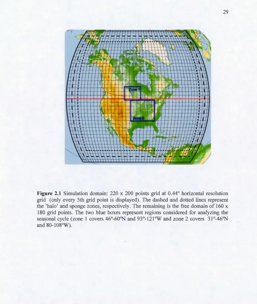
The impacts of LUC during the summer season are presented in Figure 2.4. The
differences in LAI between CRCM5_LUC and CRCM5_PV are statistically
significant over a larger region, covering regions with important LUC and adjoining
areas (Figure 2.4a). For southerly regions (south of 50°N), the differences are
positive, suggesting higher LAI, while for northerly regions (north of 50°N) it is
negative, suggesting lower LAI in CRCM5 _LUC compared to CRCM5 _PV. These
negative values for the northern regions are due to shorter growing season of crops,
compared to that of grass (which is year round in the model), leading to lower
average LAI values. For the northerly regions (north of 50°N) the onset (harvest)
happens later (earlier), compared to southern regions. The higher values of LAI for the regions south of 50°N is due to the higher LAI values of crops compared to grass
19
significant differences m albedo (Figure 2.4b), with albedo being higher rn
CRCM5 LUC.
The differences in albedo for surnmer are much smaller than that for winter. The
higher values of albedo in CRCM5 _LUC for the northem regions is primarily due to the lower LAI values, while for the southern regions, the noted higher values of albedo, despite higher LAI values is partly due to the drier surface soil layers due to increased evaporation. The differences in albedo are reflected in the reduced SHF
values over the central and eastern parts of the US in CRCM5_LUC (Figure 2.4c). The latent heat flux (LHF), on the other hand, appears hig_her in CRCM5_LUC due to
higher LAI for these regions. The lower SHF, and the increased LHF and associated evaporative cooling lead to cooler temperatures in CRCM5_LUC (Figure 2.4c). This
is also reflected in the TMin, TMax and in the soil temperatures (Figure 2.4f-h).
The comparison of the 10 rn wind field between CRCM5_LUC and CRCM5_PV shows statistically significant high wind magnitude values over a small region of
northeast US during winter and summer seasons (Appendice B). These high values could be a response to the replacement of broadleaf trees with crops. In central US, statistically significant changes in wind magnitude are observed, where lower values are displayed in both seasons. However, the differences are smaller than 0.5 m/s and
0.25 m/s for summer and winter, respectively (Annexe A). These two small zones, northeast and central US, present changes in the wind field but do not show that LUC impacts circulation and are not indicative of a LUC influenced teleconnection over North America.
2.3.2 Analysis of Average Annual Cycles
Results presented above show that the statistically significant differences are mostly
collocated with regions of important LUC. Therefore, two regions, zone 1 and zone 2, are defined to look carefully at the differences in the annual cycles in CRCM5_LUC and CRCM5 PV of selected surface variables. Zone 1 covers 46°-60°N and
94°-114.5°W, and includes central Canada and a small region of northern central US. Zone 2 covers 31 °-46°N and 80-1 03°W, which includes most of the LUC regions in the central to eastern US (Figure 2.1).
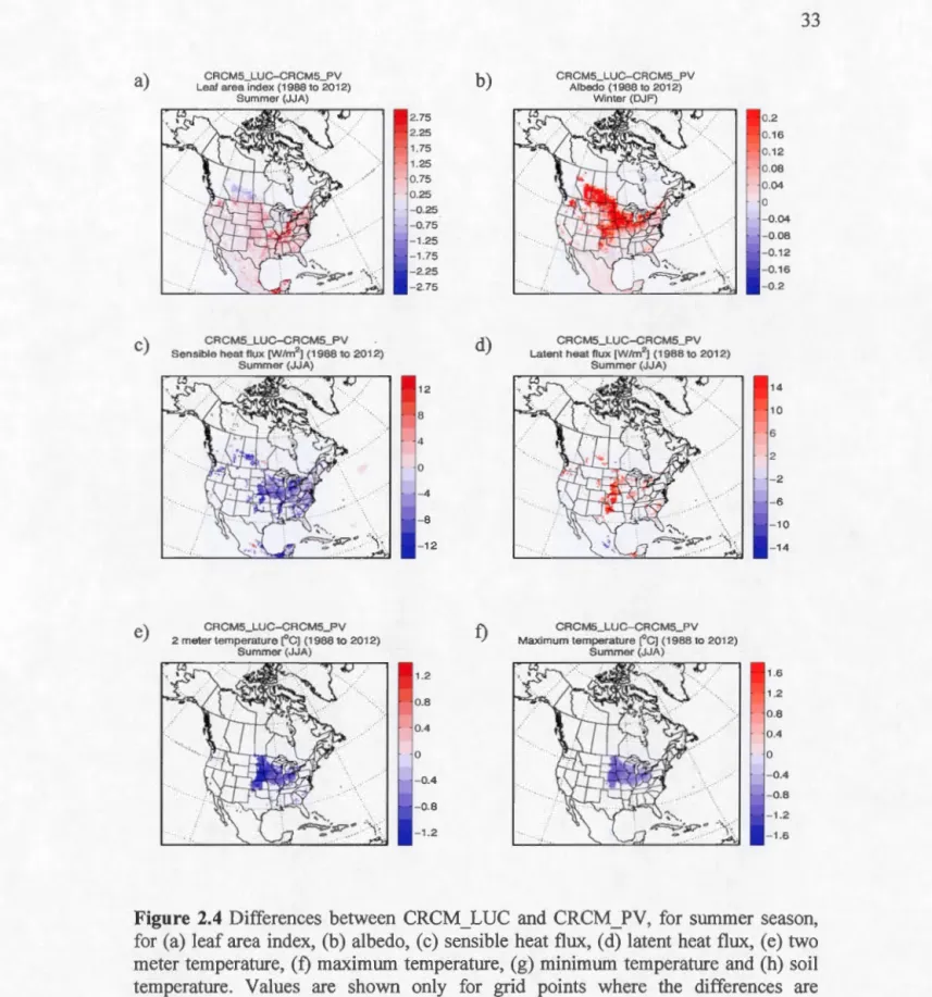
In order to evaluate the LUC effects over these zones, grid points with crops in the CRCM5_LUC simulation in zones 1 and 2 are selected for analyzing the mean annual cycles in both CRCM5_LUC and CRCM5_PV simulations (Figure 2.5, 2.6 and 2.7). The annual cycle of albedo shows high values from January to April and from October to December and low values during the summer months, as expected, due to the presence of snow during the late winter to early spring seasons. Both zones present the same tendency, but zone 2 has lower values in winter compared to zone 1,
given its southerly location (Figure 2.5a). The annual cycle of the differences between the two simulations, suggest larger differences during the fall to spring periods (Figure 2.5b ). Differences in albedo between the two simulations are larger for zone 1 compared to zone 2, mainly due to the larger differences in snow water equivalent over zone 1 (Figure 2.5b and f). This relationship reinforces the snow-albedo feedback, as suggested before, during winter months (Figure 2.5a ande). The higher snow water equivalent values in CRCM5_LUC leads to higher spring peak flows for both zones as shown in Figure 2.6a. The differences are again larger for zone 1 compared to zone 2 due to its northem location (Figure 2.5b ). Generally higher runoff values are noted for ail months, except for summer and begining and
end of fall and spring, respectively. The maximum differences in runoff occur at different times for the two zones (Figure 2.6b ). This is due to the fact that snowmelt
starts one month earlier in zone 2 because of its geographie location. As for the period of May to October, as discussed earlier, the differences between the two imulations are near zero since runoff is mostly coming from baseflow and surface runoff during precipitation events. Note that no significant differences are noted for precipitation for the two zones.
21
Figme 2.5c shows the annual cycle ofT2M. The comparison between CRCMS_LUC
and CRCMS_PV shows that the cooling effect ofLUC occurs throughout the year; it is however higher from January to April, with differences higher than 0.9°C (Figure 2.5d). The cooling over this period is related to high albedo and snow water equivalent values in CRCMS_LUC as already disccussed (Figure 2.5). On the other hand, the CRCMS_LUC cooling trend observed from May to September is related to higher evapotranspiration values, which is particularly noticeable over zone 2 (Figure 2.5a, b, 2.6c and d). Maximum evapotranspiration is observed in June and July for zone 1 and 2, respective! y (Figure 2.6c ). As for the difference between the simulations, CRCMS_LUC for zone 2 shows higher evapotranspiration values over the period of June to November, mostly during the presence of crops over that zone. As for zone 1, the higher evapotranspiration differences are noted from June to August and are smaller than for zone 2, mainly due to shorter growing season in this zone compared to zone 2 (Figure 2.6d).
The annual cycle of integrated soil moisture shows high value during snowmelt, for both zones (Figure 2.6 e). During the warm months, there is a decreasing tendency in oil moisture as a result of high evapotranspiration (Figure 2.6e). The integrated soil moisture is higher in the CRCM5_LUC experiment for both zones. The integrated soi! moisture is generally higher for zone 1, compared to zone 2, despite the higher values of precipitation for zone 2 compared to zone 1 (Figure 2.7a). The lower values for zone 2 are related partly to the higher rate of evapotranspiration and partly due to relatively shallow depth to bed rock (figure not shown). The differences in soil moisture between CRCMS_LUC and CRCMS_PV are smaller for zone 1 (Figure 2.6f), compared to zone 2. The differences in precipitation between the two simulations are small (Figure 7b ). The precipitation is slightly higher in CRCMS_LUC during the swnmer months for zone 1 and zone 2, but the differnces are not statistically significant.
2.4 Discussion and conclusions
The biophysical effects of LUC can result in cooling or warming depending on the duration of the growing season, changes in albedo and partitioning of available energy between sensible and latent heat fluxes. The
!WO
CRCMS simulations considered in this study, with and without LUC, suggest significant impacts of LUC on the regional climate of North America. The results show a cooling effect over the LUC regions during winter and summer. The mechanisms leading to this cooling are different for the two periods. The cooling effect of LUC in winter is more than 1.4o
c.
This is mainly attributed to the high albedo values in LUC regions, which is further enhanced via snow-albedo feedback, in agreement with Bonan G. (2008), Feddeman et al. (2005) and Brovkin et al. (1999). As for the summer season, the regions with statistically significant cooling are smaller, with differences in two meter temperature values less than 1.2
o
c_
The cooling here is prima.Jily due to high (low) latent (sensible) heat flux values. The above impacts of LUC a.J·e congruent with the studies of Bonan (1997) and Oleson et al. (2004) where they report cooler temperatures over the LUCregions ofNorth America in summer season because ofhigh latent heat flux values. Two zones were analyzed to further understand the influence of LUC, one covering central Canada and the other central east US, using onJy grid points with crops in the simulation with LUC. Analysis of the seasonal cycles for bath simulations suggests that the cooling effect of LUC is present year round. The impacts of LUC on evapotranspiration and sail moisture are also year round. However, the impact on runoff is mostly restricted to snowmelt season. It should be noted that the precipitation differences are not statistically significant. This could be due to the weak sail moisture-precipitation coupling over the Great Plains in CRCMS as discussed in Dira et al. (2014). Furthermore, the absence of irrigation m
,~
23
CRCM5_LUC, could also contribute to the non-signi:ficant differences m
precipitation between the two simulations.
In this study, only croplands were used to represent human activity over North
America and the biophysical effects of thjs LUC were evaluated. The influence of
inigation over croplands is not included, but it would be important to implement it in
future regional climate simulations. Studies, however, have been done using GCMs
that include irrigation. For example, Haddeland et al. (2006) in their study used an
irrigation scheme over Colorado and Mekong River basins and found that latent heat
flux increases along with a decreases of temperature, over these areas. Trus was
identified over large fraction of grid cells where the irrigation was implemented. Lo
and Famiglietti (20 13), in their study using a regional climate mode! with irrigation
over the central valley of Califorrna, showed that iuigation leads to an increase in
evapotranspiration leading to net land surface cooling. Another important influence
was an increase in precipitation, mainly in summer, enhancing the monsoon rainfall
over the southwest US.
It must also be noted that sub-grid lakes and wetlands were not considered in trus
study. These should also be included in futures studies. Furthermore, future studies
should also take into account pastures, urban areas and disturbances such as fire. It is
also important to consider LUC in transient climate change simulations with regional
climate models. Currently, many regional clirnate models do not include trus. Studies
with global climate models have shown that urballization leads to wruming at
regional and local scales, pastures lead to cooling over temperate zones and :fires lead
to decreases in precipitation due to reduced evapotranspiration [Boysen et al., 2014;
He et al., 2007; Cochrane & Laurance, 2008]. CRCM5 transient climate change simulations, including land use change will be perfonned in the near future to investigate the biophysical effects of LUC on projected changes to the urface clirnate
Acknowledgments
This work was supported by the Natural Sciences and Engineering Research Council
of Canada Discovery Grant (NSERC-DG) and the Canada Research Chairs progrmn.
Arlette Chacôn was the recipient of a CREA TE - Training Pro grain in Climate Sciences graduate fellowship. Computational resources were provided by Centre pour l'Étude et la Simulation du Climat à l'Échelle Régional (ESCER) at Université
du Québec à Montréal (UQAM) and Calcul Québec, an organization of Québec
Universities brought together by Advanced Research Computing (ARC). We would
like to thank Katja Winger and Luis Dumte for theit· technical assistance regarding
the CRCMS simulations, Oleksandr Huziy and Cmnille Garnaud for their assistance with procesing datasets and Gulilat Tefera Diro for useful discussions.
CHAPITRE III
CONCLUSION
Des études récentes sur les impacts des changements de l'utilisation des terres qui utilisaient des modèles climatiques globaux ont démontré que ces impacts sont propres à la localisation de la région étudiée. C'est pourquoi plusieurs études avec des modèles climatiques régionaux ont été menées sur différente régions afin de comprendre les impacts locaux des changements de 1 'utilisation des terres. Dans cette étude, nous avons évalué les impacts des changements de l'utilisation des terres en Amérique du Nord en utilisant la cinquième génération du Modèle Régional Canadien du Climat (MRCC5).
Pour ce faire, deux simulations du MRCCS ont été effectuées sur une grille couvrant essentiellement l'Amérique du Nord à 0,44° de résolution hmizontale (- 50 km), pour la période de 1979 à 2012. Les deux simulations se différencient de par les ensembles de données fournissant la couverture terrestre. La première simulation, nommée CRCMS _PV, est réalisée avec la végétation potentielle, ou en d'autres termes, la végétation qui existerait si la région était sans activités humaines. L'ensemble de doru1ées de végétation potentielle utilisée dans cette étude suit Ramankutty et Foley (1999), qui comprend 15 types de végétation, disponibles à une résolution temporelle de 5 min. La deuxième simulation, nommée CRCM5_LUC, représente l'utilisation actuelle des terres, créé par la fusion des données de végétation potentielle et des
données de teiTes cultivées qui représente les terres agricoles de 1 'année 2000 suivant
l'étude de Ramankutty et al. (2008). Les deux simulations sont pilotées par
ERA-Interim aux frontières latérales pour la période de 1979 à 2012 et les neuf premières
années correspondent au spin-up de la simulation et ne sont donc pas considérées
dans l'analyse de cette étude.
Les deux simulations du MRCCS montrent que le changement de la végétation
potentielle en terres cultivées influence le climat régional de l'Amérique du Nord,
avec des températures plus basses sur les régions des changements de l'utilisation des
terres pendant l'hiver et l'été. Les mécanismes conduisant à ce refroidissement sont
différents pour les deux saisons. L'effet de refroidissement dû aux changements de l'utilisation des tenes en hiver est de 1,4 °C. Ceci est principalement attribuable à la
rétroaction positive entre les valeurs plus élevées de l'albédo et la neige dans les
régions des changements de l'utilisation des terres. Pour la saison estivale, le refroidissement dû aux changements de l'utilisation des terres est moins important,
avec des différences de 1,2
o
c
dans la température à 2 mètres. Ceci estprincipalement dû à des valeurs élevées (faibles) des flux de chaleur latente
(sensible). Les impacts des changements de l'utilisation des terres sont en accord avec
les études de Bonan (1999) et Oleson et al. (2004), où ils rapportent des températures
plus basses sur les régions des changements de 1 'utilisation des terres en Amérique du
Nord pour la saison estivale en raison des valeurs plus élevées des flux de chaleur
latente. ·
Deux sous-régions ont été analysées afin de mieux comprendre l'influence locale des
changements de l'utilisation des tenes. L'une couvre le centre du Canada et l'autre le
centre-est des États-Unis (Figure 2.1). L'analyse des cycles saisonnjers pour les deux
simulations suggère que l'effet de refroidissement des changements de 1 'utilisation des terres est présent toute l'année. Les impacts des changements de l'utilisation des
27
présents toute l'année. Cependant, l'impact sur le ruissellement est principalement
limité à la saison de la fonte des neiges.
Dans cette étude, seules les terres cultivées ont été utilisées pour représenter l'activité
humaine en l'Amérique du Nord et seuls les effets biophysiques des changements de
1 'utilisation des terres ont été évalués. Des études futures devraient également prendre
en considération les pâturages, les zones urbaines et les perturbations comme les
incendies. Il est également important de considérer les impacts des changements de
1 'utilisation des tenes dans un contexte de changements climatiques avec des modèles
climatiques régionaux. Des études avec des modèles climatiques globaux ont montré
que l'urbarusation peut conduire à un réchauffement local, les pâturages peuvent
conduire à un refroidissement sur les zones tempérées et les feux de forêts peuvent
entraîner une baisse des précipitations en raison d'une évapotranspiration réduite
[Boysen et al., 2014.; He et al., 2007; Yao et al., 2015 et Cochrane et Laurance,
2008]. Les études futures devraient donc analyser les changements projetés des effets
biophysiques des changements de 1 'utilisation des terres sur l'hydrologie de surface et
Figure 2.1 Figure 2.2 Figure 2.3 Figure 2.4 Figure 2.5 Figure 2.6 Figure 2.7 FIGURES Sub-section 2.2.2 : Methodology Section 2.3 : Results
Section 2.4 : Summary and conclusions Sub-section 2.2.2 : Methodology Section 2.3 : Results Section 2.3 : Results Section 2.3 : Results Section 2.3 : Results Section 2.3 : Results
29
Figure 2.1 Simulation domain: 220 x 200 points grid at 0.44° horizontal resolution grid ( only every 5th g:rid point is displayed). The dashed and dotted lines represent the 'halo' and sponge zones, respectively. The remaining is the free domain of 160 x 180 grid points. The two blue boxes represent regions considered for analyzing the seasonal cycle (zone 1 covers 46°-60°N and 93°-121°W and zone 2 covers 31°-46°N and 80-1 08°W).
a)
b)
c)
d)
CRCMS PV CRCMS LUC
Figure 2.2 a) Needleleaf, b) broadleaf, c) crop and d) gra s fractional areas for
CRCM_PV (left panels) and CRCM_LUC (right panels).
09 0.8 0.7 0.6 0.5 0.4 03 02 01
a) c) e) CRCM5_LUC-CRCM5_PV Leal area index ( 1988 to 2012) Winter (DJF) CRCM5_LUC-CRCM5_PV Sensible heat flux [W/m2] (1988 to 2012) Winter (DJF) CRCM5_LUC-CRCM5_PV
Maximum temperature I"CJ (1988 to 2012)
Winter (DJF) b) d) f) ··./. CRCM5_LUC-CRCM5_PV Albedo ( 1988 to 2012) Winter (DJF) CRCM5_LUC-CRCM5_PV 2 meter temperature [0 C] (1988 to 2012) Winter (DJF) CRCM5_LUC-CRCM5_PV
Minimum temperature ["C] (1988 to 2012)
Winter (DJF) 0.08 0.04 0 -0.04 -0.08 -0.12 -0.16 -0.2 31
Figure 2.3 Differences between CRCM_LUC and CRCM_PV, for winter, for (a) leaf
area index, (b) albedo, (c) sensible heat flux, (d) maximum temperature, (e) minimum
temperature, (f) two meter temperature, (g) height of the bounday layer, (h) snow
depth and (i) runoff. Values are shown only for grid points where the differences are
g)
i)
CRCM5_LUC-CRCM5_PV
Height boundary layer [m] (1 988 to 2012)
Winter (DJF) CRCM5_LUC-CRCM5_PV Runoff [mm/day] (1988 to 2012) Spring (MAM) Fi gu re 2.3 ( continued) h) CRCM5_LUC-CRCM5_PV Snow water equivalent [cm] (1988 to 2012) Winter (DJF)
a) c) e) CRCM5_LUC-CRCM5_PV Leaf area index (1988 to 2012) Summer (JJA) CRCM5_LUC-CRCM5_PV Sensible heat flux [W/m2] (1988 to 2012)
Summer (JJA) CRCM5_LUC-CRCM5_PV 2 meter temperature ["C) (1988 to 2012) Summer (JJA) 1.75 1.25 0.75 0.25 -0.25 -0.75 -1.25 -1.75 -2.25 -2.75 b) d) f) CRCM5_LUC-CRCM5_PV Albedo (1988 to 2012) Winter (DJF) CRCMS_LUC-CRCMS_PV Latent heat flux [W/m2] (1988 to 2012) Summer (JJA) CRCM5_LUC-CRCMS_PV
Maximum temperature ["C) (1988 to 2012) Summer (JJA)
33
Figure 2.4 Differences between CRCM_LUC and CRCM_PV, for summer season, for (a) leaf area index, (b) albedo, ( c) sensible heat flux, ( d) latent heat flux, ( e) two
meter temperature, (f) maximum temperature, (g) minimum temperature and (h) soil
temperature. Values are shown only for grid points where the differences are
g) CRCM5_LUC-CRCM5_PV Minimum temperature ('C] (1988 to 2012) Summer (JJA) Figure 2.4 ( continued)
h)
CRCMS_LUC-CRCMS_PV Sail temperature ('C] (1988 to 2012) Summer (JJA)a) c) e) ü Q.... Q) :; (ij Iii Q. E Q) f-Iii (ij ~ ;: 0 c
Avg. annual cycle of Albedo (1988-2012)
02 03 04 05 06 07 08 09 10 11 12
Months
-+-LUC-Zone1 -+-LUC-Zone2-+-PV-Zone1 -+-PV-Zone2
Avg. annual cycle of temperature (1988-2012)
02 03 04 05 06 07 08 09 10 11 12
Months
-+-LUC-Zone1 -+-LUC-Zone2-+-PV-Zone1 -+-PV-Zone2
Avg. annual cycle of snow water equivalent (1988-2012)
Cl) 2
0
01 02 03 04 05 06 07 08 09 10 11 12
Months
-+-LUC-Zone1-+-LUC-Zone2-+-PV-Zone1-+-PV-Zone2
b) d) f) 'E ~ ë Q) ~ ·:; cr w Q;
~
;: 0 c Cl) 0.06 . 'Dili. annual cycle of Albedo
CRCM5_LUC-CRCM5_PV 1988-2012
35
0.04 ! .,. 0.02 .. 0~0~1-702~~~~~~~~~~~11~1~2 -2.7Diff. annual cycle of temperature
CRCM5_LUC-CRCM5_PV 1988-2012
-3 01 02 03 04 05 06 07 08 09 10 11 12
Months -+-Zone1 -+-Zone2
Diff. annual cycle of snow water equivalent
CRCM5_LUC-CRCM5_PV 1988-2012
02 03 04 05 06 07 08 09 10 11 12
Months
-+-Zone1 -+-Zone2
Figure 2.5 Left panels: average seasonal cycle for the 1988-2012 period for a) albedo, c) two meter temperature and e) snow water equivalent. Right panels:
difference between CRCM5_LUC and CRCM5_PV seasonal cycle for b) albedo, d)
a) c) e) 450 400 350 >: "'300 :!;?
ê
250 ;; 200 0 3 150 a: 100 50Avg. annual cycle of runoff (1988-2012)
.;. ... .; . -~ ... ! .
02 03 04 05 06 07 08 09 10 11 12
Months
--+-LUC-Zone1 -+-LUC-Zone2--+-PV-Zone1 -+-PV-Zone2
Avg. annual cycle of evapotranspiration (1988-2012)
4rr--~~-r-,--~-r~--~~-. --r-~3.5 :!;? E 3 E -; 2.5 0 ~ 2 o. ~ 1.5 ~ 1
"'
dJ 05 04 05 06 07 08 09 Months--+-LUC-Zone1 -+-LUC-Zone2--+-PV-Zone1 -+-PV-Zone2
Avg. annual cycle of integr. sail moisture (1988-2012)
b)
d)
f)
Diff. annual cycle of runoff
CRCM5_LUC-CRCM5_PV 1988-2012 200,.--~--.--.----.-~--,----,--,.-~---.---.-, 175 . . . .. 150 >: :!2 125 ~ 100 ;; 7S 0 c ::J a: . ,, . -~ ... . ... . .. ····: -2S 01 02 03 04 os 06 07 08 09 10 11 12 Months --+-Zone1 --+-Zone2
Diff. annual cycle of evapolranspiration CRCMS_LUC-CRCMS_PV 1988-2012 0.2S,.----.-~--,----,----,--,---,----,--~-.---r-, >: 0.2
"'
~ 0.15 É. 0.1 .Q 0.05 "§ o. g? -D.OS ~ -{)1 0 g.-D.1S > w -{).2 -D.2s'Lo~1--=o'=""2 -0:':3--::0L-4 ----:':os--::oe':-='=o7:-:o'=-8 ----:':o9:--:1'=-o----:'"11:--:1':--2 Months --+-Zone 1 -+-Zone2Diff. annual cycle of integr. sail moisture CRCMS_LUC-CRCMS_PV 1988-2012 181,...-,-,--,-,-,-,---,----,--~,-,--, %16 .. . .. o, 14 ~ 8 "ë 6 (/) ti, 4 Q) Ë 2 0 01 .,. 02 03 04 os 06 07 08 09 Months --+-Zone 1 -+-Zone2 10 11 12
Figure 2.6 Left panels: average seasonal cycle for the 1988-2012 period for a) runoff, c) evapotranspiration and e) integrated soil moisture. Right panels: difference between CRCMS LUC and CRCMS PV seasonal cycle for b) runoff, d)
a) Avg. annual cycle of precipitation (1988-2012)
.10 0
01 02 03 04 05 06 07 08 09 10 11 12 Months
-+-LUC-Zone1 ... LUC-Zone2-+-PV-Zone1 ... PV-Zone2 b)
-6 01
Diff. annual cycle of precipitation
CRCM5_LUC-CRCM5_PV 1988-2012
37
05 06 07 08 09 10 11 12
Months -+-Zone1 ... Zone2
Figure 2.7 Left panel: average seasonal cycle for the 1988-2012 period for a) precipitation. Right panel: difference between CRCM5 LUC and CRCM5 PV seasonal cycle for b) precipitation.