Cell-based array for deep sub-micron technologies

Cell-Based Array for Deep Sub-Micron

Technologies

by

James Boe-Kian

Oey

Submitted to the Department of Electrical Engineering and Computer

Science

in partial fulfillment of the requirements for the degree of

Master of Engineering in Electrical Engineering and Computer Science

at the

MASSACHUSETTS INSTITUTE OF TECHNOLOGY

August 2003

©

James Boe-Kian Oey, MMIII. All rights reserved.

The author hereby grants to MIT permission to reproduce and

distribute publicly paper and electronic copies of this thesis document

MASSACHUSETTS INSTI WTE in whole or in part. OF TECHNOLOGY

JUL 2

0

2004

LIBRARIES

Author ...

Department of Electrical Engineerifg and Computer Science

August 13, 2003

Christd herJ. Terman

Senior Lecturer

Thesis SApervisor

Accepted by...

...

Arthur C. Smith

Chairman, Department Committee on Graduate Students

Cell-Based Array for Deep Sub-Micron Technologies

by

James Boe-Kian Oey

Submitted to the Department of Electrical Engineering and Computer Science on August 13, 2003, in partial fulfillment of the

requirements for the degree of

Master of Engineering in Electrical Engineering and Computer Science

Abstract

In this thesis I explore transistor topologies for high density cell-based arrays that al-lows for dense computation blocks, small memory cells, and strong signal drivers. This involves simulating different circuit types with HSPICE to determine ideal transistor sizes. Using Magic and the results of the HSPICE simulations, I explore transistor topologies with different ratios of nFets to pFets. An analysis on the technology shows important characteristics for digital systems and how they relate to the explored tran-sistor topologies.

Thesis Supervisor: Christopher J. Terman Title: Senior Lecturer

Acknowledgments

I would like to thank Christopher Terman for his guidance throughout this thesis project. He has helped me by teaching the material in both Computation Structures and Introduction to VLSI Systems, as well as providing support and insight through-out this project. I am very grateful for the chance to work with him. I have learned many lessons from our interactions.

It has been a pleasure meeting and spending time with friends at MIT. It has given me the chance to learn different things that MIT simple cannot teach. May we

all be together in the future.

Lastly, I would like to thank my parents, Peter and Theresia, and my two brothers, Michael and Christopher. They are always there for me when I need help, and have always shown love and support throughout my life. I certainly could not have made it through the challenging parts of my life without my family. Thanks a lot for your support!

Contents

1 Introduction

1.1 Problem Description . . . . 1.2 Prior W ork . . . . 1.2.1 Sea-of-Gates . . . . 1.2.2 Sea-of-Gates Structure for Digital and Analog Applications . .

1.2.3 Cell-Based Array Patent . . . .

1.3 General Overview . . . .

2 Circuit Types and Spice Simulations

2.1 Spice Simulations . . . . 2.2 Ideal Circuits . . . . 2.2.1 Cell-Based Logic . . . . 2.2.2 Domino Logic . . . . 2.2.3 SRAM Cell . . . . 2.2.4 DRAM cell . . . . 2.2.5 Spice Decks . . . . 2.3 Conclusion . . . . 2.3.1 Transistor Ratios . . . . 2.3.2 Transistor Sizes . . . .

3 Diffusion Topology and Routing

3.1 Magic . . . .

3.1.1 Design Rules and Technology . . . .

13 13 14 14 15 16 18 21 22 22 22 23 28 32 39 40 40 41 43 43 43

3.1.2 General Layout Issues . . . . .

3.1.3 _{Sharing Polysilicon Among Mult}

3.2 Layouts using equal number of p-type a

3.2.1 SRAM 6-T cell . . . .

3.2.2 Logic Cells . . .

3.2.3 DRAM 3-T cell

3.2.4 DRAM 1-T cell

3.3 Layouts using twice the

3.3.1 SRAM 6-T cell

3.3.2 DRAM 3-T cell

3.3.3 DRAM 1-T cell

3.4 Layouts using only one 3.4.1 SRAM 6-T cell 3.5 Conclusion . . . . 3.5.1 Standard CMOS 3.5.2 3.5.3 number of i-type and Cells n-typ one . . . . iple Diffusion . . . . nd n-type transistors . . . . .

e devices than p-type devices

-type transistor . . . . . . . . . . . . . . . . . . . . . . . . Memory Cells Domino Logic 4 Analysis 4.1 Capacitances . . . . 4.1.1 Gate Capacitance . . 4.1.2 Drain Capacitance . . . 4.1.3 Wire Capacitance . .

4.1.4 MAGIC Technology File

4.1.5 Experiments . . . . 4.2 Switching Characteristics . . . . 4.2.1 Experiments . . . . 4.3 Power Dissipation . . . . 4.3.1 Static Dissipation . . 4.3.2 Dynamic Dissipation . 44 44 46 46 49 50 54 58 58 58 59 61 61 61 62 63 64 65 66 66 66 67 68 69 72 73 77 77 78

4.3.3 Experiments . . . . 78

4.4 Supply Voltage . . . . 83

4.4.1 Experiments . . . . 83

4.5 Layout . . . . 84

4.5.1 Total Circuit Area . . . . 84

4.5.2 Circuit Overhead . . . . 85

4.5.3 Percent of Transistors Used . . . . 85

4.6 Conclusion . . . . 85

5 Conclusion 89 5.1 Current State . . . . 89

5.2 Comparisons. . . . . 90

5.2.1 Area and Performance Comparison . . . . 90

5.2.2 Different Transistor Topologies in a System . . . . 91

5.3 Predictions for Larger Systems . . . . 92

5.3.1 Routing Availability . . . . 92

5.4 Further W ork . . . . 93

5.4.1 Ocean . . . . 93

A SPICE Design Files 95 A.1 Standard Gates . . . . 95

List of Figures

1-1 Sample NOR gate layout using Ocean: Sea of Gates System. . . . . . 14

1-2 Exemplary cell arrangement in cell-based array patent. . . . . 16

2-1 Transistor circuit diagram for the nand2 gate. . . . . 23

2-2 Circuit diagram for a dual-rail XOR domino gate. . . . . 24

2-3 Gate-level diagram for a full-adder circuit. . . . . 25

2-4 Circuit diagram for a domino full-adder circuit. . . . . 25

2-5 A, B, and Carry inputs for domino full-adder . . . . 27

2-6 Clock, and Carry Out, Sum (dotted) outputs for domino full-adder . 28 2-7 The SRAM block includes the 6-T cell, a sense amplifier and write drivers. . . . . 30

2-8 The SRAM transistor chain during a read consists of the load nFet, the access nFet and the inverter nFet. . . . . 30

2-9 Word input, Write input, and Bit lines for SRAM cell . . . . 31

2-10 The 3-Transistor DRAM cell consists of a read access, write access and a storage transistor. . . . . 33

2-11 The 1-T DRAM system requires the cells, some dummy cells and a cross-coupled sense amplifier . . . . 35

2-12 Left bit-line and right bit-line(dotted) for 1-Transistor DRAM cell on a 0 and a 1 write/read . . . . 37

3-1 Diffusion pattern for transistors that share polysilicon gates . . . . . 45

3-2 6-T SRAM layout using only metal 1 . . . . 47

3-4 Layout of full-adder block . . . . 49

3-5 Layout of dual-rail XOR gate . . . . 51

3-6 Clock, and Carry Out, Sum (dotted) outputs for domino full-adder (layout version) . . . . 52

3-7 3-T DRAM layout . . . . 53

3-8 1-T DRAM bit-slice, showing 2 bits of storage per 3 columns . . . . . 55

3-9 1-T DRAM 32-bit block . . . . 56

3-10 1-T DRAM restorative sense-amp, using a cross-coupled inverter . . . 56

3-11 1-T DRAM write driver, driving the left bit-line . . . . 57

3-12 6-T SRAM cell using 2:1 of N:P ratio . . . . 59

3-13 1-T DRAM bit-slice using 2:1 of N:P ratio, showing 2 bits of storage per 3 colum ns . . . . 60

3-14 6-T SRAM cell using 1:1 of N:P ratio . . . . 62

4-1 Different types of wire capacitances . . . . 67

4-2 Layout of two squares of metal for capacitance measurement . . . . . 71

4-3 Minimum sized inverter layout . . . . 74

4-4 Circuit diagram for HSpice inverter under test . . . . 75

4-5 In (solid) and Out (dotted) port of a typical inverter of size 8/4 with no load... ... 76

4-6 In (solid) and Out (dotted) port of a typical inverter of size 8/4 with F04 load ... ... 76

4-7 Currents for typical inverter of size 8/4 with no load . . . . 80

4-8 Currents for typical inverter of size 8/4 with F04 load . . . . 82 4-9 Delay (ns) vs. Supply Voltage (V) for an 8/4 inverter with F04 load . 83

Chapter 1

Introduction

1.1

Problem Description

Today, both industry and educational institutions throughout the world use gate-array technologies to design digital systems. While the design time is minimal com-pared to companies who choose full-custom designs, gate-arrays have several draw-backs, often causing an inability to meet circuit timing and area specifications. Be-cause typically gate-arrays only have a limited selection of transistors, circuits cannot benefit from having a selection of transistor sizes to create small computation circuits and larger drive circuits. Generally, gate-arrays have large transistors for all circuits; for many systems, using larger transistors will cause blocks to run slower than circuits with a wide selection of transistor sizes. In addition, using large transistors will con-sume much silicon, costing the designer both area on the silicon that could be used for other system blocks and money for the actual cost of the silicon.

Digital designers are seeking for a median between the two extremes, allowing for a fair balance between speed, area, and design time. In this thesis we discuss diffusion topologies for transistors that allow for efficient layout and routing of common cells

1.2

Prior Work

1.2.1

Sea-of-Gates

Sea-of-gates is a specific type of approach to generalizing a digital design where a chip contains a continuous array of nFets and pFets. Unlike full-custom layout designs, sea-of-gates only require the wiring of the transistors to complete a design. However, with this limitation, the technology is still very generic. The approach to such a design begins with the formulation of a single block that consists of a small number

of transistors, and then replicate it many times on the same piece of silicon.

Ocean: the Sea-of-Gates Design System is a working CAD tool that implements a sea-of-gates example; the fishbone layout, shown in Figure 1-1, is one of the simplest topologies available in a sea-of-gates system. It is a standard pattern with alternating rows of nFets and pFets.

aU

[* K

Figure 1-1: Sample NOR gate layout using Ocean: Sea of Gates System.

The DIMES production facility in the Netherlands is capable of producing chips developed using the fishbone master image. Two other images, octagon and gatearray, serve as examples for the different features of the Ocean system.

Tools

Ocean: the Sea-of Gates Design System uses a number of different tools in its design process, listed in [3]. The next few paragraphs details a few of these tools.

Seadali is the main CAD tool used to generate layouts. This tool includes the fish, madonna, and trout programs. The first tool, fish, takes layouts and purifies them, creating a newer enhanced cell. Madonna is a partitioning based sea-of-gates placer that uses a netlist the designer provides. Although this program does not always generate the optimal layout, it can be a useful tool, especially in large systems.

Trout is the sea-of-gates router. After the designer lays out and labels some cells, trout will route these cells together based on the SLS file linked to the project. If

the designed feeds the router enough information, trout will respond successfully if there is a route available for the particular cell layout.

After generating a layout, it is necessary to perform an extraction of the layout in order to simulate the behavior of the circuit. Ghoti is a script that purifies sea-of-gates extracted circuits. It takes a layout and removes the unnecessary transistors from the circuits. Space performs the actual extraction and generates a file readable

by simeye, the simulation tool provided by Ocean.

1.2.2

Sea-of-Gates Structure for Digital and Analog

Appli-cations

Phillipe Duchene and Michel Declercq, in [1], describe a generalized sea-of-gates struc-ture that is suitable for a number of digital and analog applications. The paper gives a general description of the sea-of-gates concept, including the current limitations of a sea-of-gates implementation. The basic template for their structure includes 2 nFets and 1 pFet per transistor column.

In their new structure, they argue that a random logic design reduces the number of routing channels, since cells from a library would not be specific to the intended application. They also argue that optimization of regular circuits such as RAMs, ROMs or PLAs is possible. The article further describes the key features of their

design including their reasoning for a 2:1 nFet to pFet transistor ratio, as well as their transistor and grid spacing sizing.

The last sections of the article present the results of their experiments. It compares circuit density and electrical performance of different types of circuits. They compare between sea-of-gates, gate array, standard cell and full-custom designs. Full-custom layouts excluded, sea-of-gates consume the least amount of circuit area compared to other design styles; on the average, a typical circuit consumes twice the area as a

symbolically generated full-custom layout.

1.2.3

Cell-Based Array Patent

A44GMND on ... ... .. .

N

E

7~X~

myoI

poly

nFet

Figure 1-2: Exemplary cell arrangement in cell-based array patent.

Iranmanesh et al. received a patent in January 2001 titled Cell based array having compute drive ratios of N:1 [2]. This patent approaches a unique topology allowing for compact computation circuitry yet providing larger transistor sizes for the high

CQrA

drive needed elsewhere.

The patent summarizes the invention by describing and providing diagrams for the topology. It features groups of small transistors that allows for computation, while providing a pairs of larger transistors necessary to drive higher capacitive loads. An analysis of the system describes how to improve performance, and explains the power distribution through the layout.

Figure 1-2 shows the cell arrangement for this particular invention. Notice that transistors are grouped into columns, and in each column of substrate, there are 4 pFet transistors are 4 nFet transistors. Looking at the last column of transistors to the right of the M4 VDD node, we see from top to bottom and left to right: 2 large pFet transistors, 2 small pFet transistors, 2 large nFet transistors, and 2 small nFet transistors. The claim of this patent is that the smaller transistors are useful for

compute transistors, and the larger ones are used for drive transistors.

For example, suppose a digital designer needed to design a 16-bit adder circuit. In this particular case, the computation circuit would be the different full-adders connected together. The nodes that represent the solution of the 16-bit adder would require drive transistors to be able to drive the next stage of the system. For the full-adders in these circuits, the smaller pFets and nFets are more suitable than the larger ones since these transistors will operate the fastest. Additionally, since these are in the middle of a computation circuit, there is no need to drive a huge capacitive load, so a small transistor would be the ideal size. However, if the system uses the same transistors for the output drive, then the adder would not be able to drive the next stage, and the system would suffer a large time delay.

There are a total of 8 transistors in each "transistor column." In Figure 1-2, there are 4 transistor columns shown. Having these columns separate does have some benefits, although there are some disadvantages as well. The benefit is that there is an option of having current flow or not between the diffusions across the columns. However, the disadvantage is that if three transistors need to be in series, an additional transistor can fit in between the two columns; in this diffusion layout, multiple transistors in series can be less efficient than other layouts.

1.3

General Overview

The goal of this project is to design a diffusion topology that allows for both dense computation cells and dense memory cells. This topology should demonstrate in-creased efficiency in speed and area over a standard gate-array layout. The main steps towards discovering this optimal topology are HSPICE simulations and Magic layout and extraction. After a number of iterations, a final circuit extraction can provide data for a circuit analysis to find limitations on the diffusion technology tested.

The first stage towards designing an efficient diffusion topology is to consider the different type of cells that a digital designer would need in his toolkit. From simple NAND and NOR gates to more complicated domino gates, SPICE simulations will verify correct sizing of the transistors to make ideal circuits when an unlimited number of transistors sizes are available. In addition to static and domino gates, it is important to look at six-transistor SRAM cells, three-transistor DRAM cells and one-transistor DRAM cells. Since most digital systems need some sort of memory elements, testing these cells will allow nearly full coverage of the type of cells a designer would need to design any arbitrary system.

The second stage begins to look at specific transistor topologies. To consider a number of different possible layouts, Magic allows quick editing of the diffusion and polysilicon. The main steps in this stage is to lay a specific topology, test a few circuits and measure the results. These results would be either some timing constraints or space constraints. Space constraints are easily measurable by the area a sample circuit consumes in Magic. Timing constraints on the other hand, require circuit extraction and a spice simulation. Therefore, testing on this second stage may require several iterations of SPICE simulations.

The third stage analyzes a specific transistor topology and focuses on specific characteristics of different circuits. From the previous stages, this thesis already considers timing issues and efficient use of silicon area. However, in this analysis stage, more detail is necessary: for timing, this stages considers gate delay as well

as memory reads and writes. These delays are important, since they are the major factors that limits a system from operating at a higher frequency. To be more specific regarding efficient use of silicon area, gates/mm2 is a measurable quantity that can compare and contrast different transistor topologies. However, there are other factors, such as different types of capacitances, power, and leakage current. These factors are all key issues towards designing a digital system.

Chapter 2

Circuit Types and Spice

Simulations

This chapter presents a number of circuit types important for designing an arbitrary digital system. It outlines some of the advantages and disadvantages for certain types of circuits. SPICE simulations on these idealized circuits will provide a set of useful timing criteria. Iterations on different transistor sizes will help to choose useful transistor sizes based on comparisons to the best possible circuits given the technology system uses. These types of circuits will be refered to as "ideal" for the

remainder of this chapter.

Each type of circuit has an "ideal" transistor configuration, as well as appropriate sizes for each transistor. Of course, there is a minimal number of transistors neces-sary for each circuit. However, more importantly, timing parameters are important to consider, since a large part of designing an ideal circuit is to optimize timing con-straints. Balanced rise and fall times are best for gates; however, it is very important to consider shorter times. For memory circuits, transistor sizes are important because slight variations in size can make a large difference in voltage levels, and therefore, the amount of time necessary to perform a read operation.

2.1

Spice Simulations

Since the final diffusion topology should be general, the next step is to encode each circuit into SPICE to be able to determine the best set of transistor sizes to build the circuits described above. Though it will be impossible to replicate the circuits due to simulation limitations, the transistor sizes should be a compromise between all the different types of circuits so that no circuit is much more efficient as any other. Such a condition would lead to bottlenecks; a system with highly efficient computation circuits but weak memory circuits could result in a system that spends too much time performing memory accesses.

The best approach for determining transistor sizes is to perform an analysis on the different types of circuits. Dense computation circuits will require no large transistors, while memories do require some large transistors for the reads and writes. One other factor is that two medium-sized transistors can be equivalent to a larger transistor. Therefore, circuits with larger drivers can make use of medium-sized transistors; this allows some sort of flexibility.

A more detailed description on the SPICE file format is provided at the end of

the chapter, and SPICE files used in this chapter are provided in Appendix A.

2.2

Ideal Circuits

A varied selection of CMOS circuits will allow for a generalized comparision to select

the best transistor size set. The circuit types will include cell-based logic, domino logic, and several types of memory cells and sense amplifiers.

2.2.1

Cell-Based Logic

Cell-based logic is composed of several main types of logic: simple gates, synthesis gates, and drive inverters. Simple gates (inv, mux2, nand2, nand3, nand4, nor2, nor3, nor4, and xor2) are gates used by a synthesizer as well as a person to build circuits. Synthesis gates (aoi2l aoi22, aoi211, oai2l, oai22, oai211) are larger pieces

of logic that a synthesizer would use to piece together logic equations. Inverters come in many different widths; the larger ones are drive inverters intended to drive large capacitances. Lastly, there are many types of special-purpose circuits such as multiple versions of d-flipflops and d-latches to use in different parts of a design.

T

A B

A nand B B

A

Figure 2-1: Transistor circuit diagram for the nand2 gate.

For most elements in this library, the amount of current flowing through the pull-up and pull-down network determines each transistor size. For example, assuming that the electrons have a mobility twice that of holes, the nFets in Figure 2-1 should be the same size as the pFets. This is because the current must flow through two nFets when the circuit is pulled down; while at the minimum, current will flow through a single pFet. This will balance the pull-down and pull-up delay time.

2.2.2

Domino Logic

Domino logic works differently than standard logic because it relies on a clock to precharge and evaluate a cascaded set of dynamic logic blocks[7]. The name "Domino Logic" is an analogy to falling dominos; when dominos are stacked in a row, knocking one domino down causes other dominos to fall. A gate that uses domino logic consists of a single pFet and the logic encoded into the nFet. When the clock is low, the pFet precharges the output node. When the clock is high, the evaluate nFet enables the pulldown path, allowing the nMOS transistors to conditionally discharge the output

node.

Figure 2-2 demonstarates a simple dual-rail XOR domino gate. As mentioned, when CLK is high, the output node charges. When CLK is in the low phase, a pull-down path is available as long as A B or A B is true for the XOR, and the opposite for the XOR.

CLK CLK-A xor B A xor B B B B A A CLK

Figure 2-2: Circuit diagram for a dual-rail XOR domino gate.

Because domino circuits precharge and conditionally discharges the output node, it is necessary to have inputs rise monotonically during the evaluation phase. If an operation requires a non-monotonic function such as XOR, it will be necessary to use dual-rail domino logic. This way, a signal and its complement will stablize and remain constant before the evaluation phase begins.

Figure 2-3 demonstrates a gate-level implementation of a full-adder. It consists of two XOR gates, two AND gates, and an OR gate. The XOR of the three inputs, A, B, and C7,, generates the Sum output. The Ct is determined by a majority circuit based on the three inputs.

Without using dual-rail XORs, the X input, shown in Figure 2-3, falls during evaluation. Therefore, it is necessary to implement both the X and X using a dual-rail XOR as the first XOR to properly implement the full-adder. The circuit uses only positive logic, which is important, since each stage requires a buffer inverter output. It includes two XOR gates, a XNOR gate, two AND gates and an OR gate. The

full-adder takes advantage of dual-rail domino logic, since the second XOR requires both A E B and A E B to implement the sum.

A

B

Cout

Cin

Figure 2-3: Gate-level diagram for a full-adder circuit.

CLK-S CLK Ci ] Cout CLK CLK CLK -CLK _-d CLK CLK B B B a AA Cin B CLK CLK CLK

Domino logic is advantageous over static logic because the circuits take up less area, and parasitic capacitances are smaller, resulting in faster gates because of the reduction in self-loading. Since timing constraints can focus specifically on the falling edges of output nodes, an output inverter can be designed to detect a falling transition earlier than cell-based logic. Because of this, glitch free operation is possible by design. In addition, the elimination of the pullup short-circuit current saves time and energy. Figure 2-5 shows the input waveforms for the domino full-adder circuit shown in Figure 2-4. This demonstrates a number of test patters to show the functionality of the circuit. The three waveforms show the A, B, Ci, inputs.

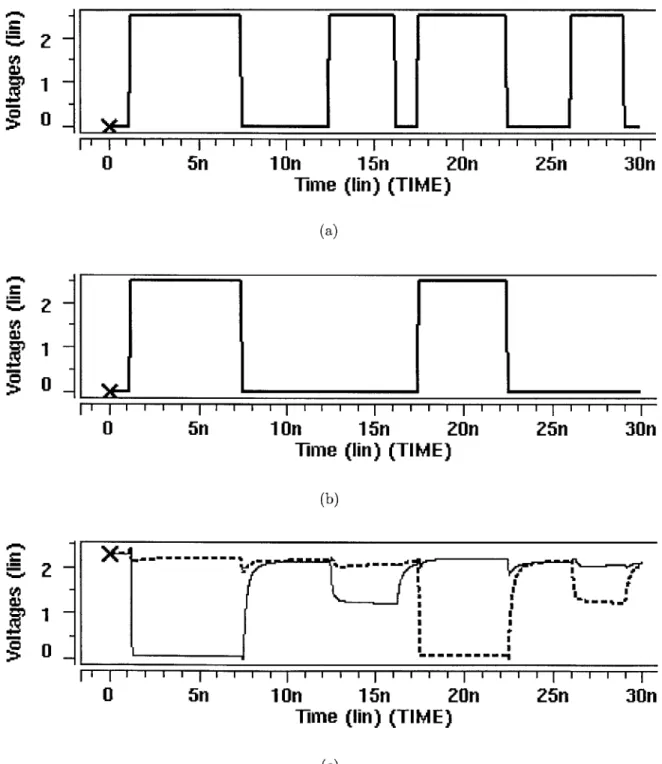
Figure 2-6 shows the relationship between the clock signal in (a) and the output signals C0st and S in (b). On the low phase of the clock, both output signals are set

to low. Next, based on the logic's functionality, each output signal is conditionally set to high. After the first discharge that occurs at about t = 1.0 ns, the values of

Cout in the next 6 clock cycles are 1, 1, 0, 1, 0, and 1. For S, the output values are

I I I 0J L - - -I -- L > -- - - - -- -- -- -0 1 I - - - - - - - - - - -

-0

2n

4n

6n

On

Time (Iin) (TI ME)

(a)

- - - -- - - - r - - - - - - -i - - - - - - I - - - - - - - r

--- -- - - - - -- - - -

-0 2n 4n 6n On

Time (Iin) (TIME)

(b

I I I I I I I I I I I I I I I I I I I I I I I I I I III I I I I I I I I I

0 2n 4n 6n On

Time (Iin) (TIME)

(a)

2

---

--0 1

0 2n 4n 6n On

Time (Iin) (TIME)

(b)

Figure 2-6: Clock, and Carry Out, Sum (dotted) outputs for domino full-adder

2.2.3 SRAM Cell

Since memories often occupy large areas in a digital layout, SRAM cells are important in the consideration of a diffusion topology. The standard six-transistor SRAM cell stores a single bit of memory using cross-coupled inverters. While this loop is stable, it is easy to change the value by driving one of the nodes with a strong transistor. While one of the major issues is the size of the actual cell, the write driver and the sense amplifier are also important modules in the SRAM system. The two functions necessary to consider are the write and read cycle.

The SRAM undergoes a write cycle when the write signal is asserted. The write and write-data transistors will drive bit and bift to Vss and VDD - Vt, depending on

the value of write-data. Since the write transistors will be larger than the transistors in the cross-coupled inverter, the write transistors will overpower the transistors in the loop, causing the memory cell to flip its state.

The SRAM's read cycle occurs when the word line is asserted. Since the bit lines need to be either charged or discharged to attain a certain voltage, the bit-line pullups transistors server to provide this charge. These transistors can be permanently on, or turned on when reading or writing. Using a precharge, rather than keeping the transistors on will save power, since the circuit can be shut off when not in use.

At this time, the two access transistors will cause either the bit or bit lines to change depending on the state of the inverters. The voltage pulled down in either bit line is dependent on the ratios of nFets in the pulldown path; the precharge, access, and one of the cross-coupled transistor pulldown transistor.

While this voltage change is too small for a standard gate to properly detect, a sense amplifier can amplify the small change to cover the full range. This sense amplifier is a differential amplifier that amplifies slight diverging changes in the bit and bit line.

VDD or precharge word word --- ---bit-line pullups bit 6-T Memory Cell Differential Sense Amplifier write write writedata

Figure 2-7: The SRAM block includes the 6-T cell, a sense amplifier and write drivers.

VDD

or load

precharge

access

> to feedback inverter

mem value inverter pulldown

Figure 2-8: The SRAM transistor chain during a read consists of the load nFet, the access nFet and the inverter nFet.

bit

.5

Is

I

Time (Iin) (TIME)

(a)

o

Time (fin) (TIME)

(b)

X -

---0

on

Time (fin) (TIME)

(c)

Figure 2-9: Word input, Write input, and Bit lines for SRAM cell

2

1 0

1

0

When choosing transistor sizes for an SRAM, there are some key points to con-sider. First, the six transistors in the memory cell should be minimized, since the majority of the memory area will be these cells. Second, the bit and bit lines will need to change quickly to decrease access time, and have a larger change in voltage to speed up the sensing. The last point is that a read operation should not flip the selected cell.

Figure 2-9 shows the word and write inputs for the SRAM cell. It also shows the two bit lines that change based on the current value stored in memory and the state of the inputs. On the first write pulse, the system writes a 0 into the memory. The second assertion of the word signal results in the bit line value of approximately

1.5 V. The second half of the simulation performs a similar task, but it writes a 1

into the memory. As a result, rather than the bit line dropping to about 1.5 V, the bit lines drops.

2.2.4

DRAM cell

Dynamic RAM cells have an advantage over static RAM cells because they take up much less space. There are a number of useful DRAM cell configurations, usually denoted by the number of transistors in the cell. This next section describe a 3-transistor and a 1-3-transistor DRAM cell.

DRAM cells have a number of disadvantages, including the necessity to refresh bits, and the susceptibility of the memory system to noise. This is because DRAM cells rely on charge storing in the system to store data; charge storing leads to charge leakage, and therefore, a restorative procedure is necessary to retain memory for long periods of time. While some systems use trench capacitors as storage elements, a sea-of-gates system such as this one will need to use gates of transistors to serve as the storage capacitors.

Three-transistor cell

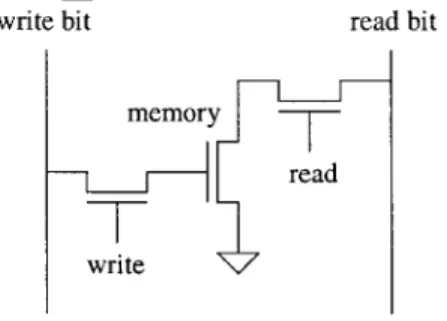
The three-transistor DRAM cell consists of a write access transistor, a memory tran-sistor, and a read access transistor. Like the SRAM cell, there are two functions to consider: the read and the write cycle.

The write access transistor enables the system to "permanently" trap charge to turn on the memory transistor. This charge remains there until the system writes a 0, that is, draining the charge, and turning the transistor off. In a true system, there is charge leakage, and the stored charge will not remain there forever; therefore, the system will have to rewrite the data to retain the charge. The leakage occurs across the gate, as well as through the access transistor. Because of charge leakage, it is beneficial to have the largest capacitance possible to charge and discharge. For this reason, using any unused transistors as a storage element would be beneficial, as demonstrated in the next chapter's description of the three-transistor cell.

write bit read bit

memory

-read

write

Figure 2-10: The 3-Transistor DRAM cell consists of a read access, write access and a storage transistor.

The read access transistor determines the value stored in the cell based on whether the memory transistor currently has a pull-down path. If the pull-down path exists, then the read line will read low; if the pull-down path does not exist, then the read line will read VDD - Vt. Note that the read and write values are actually opposites; if

the system stores a 1, then the pull-down path is available, and the system will read a 0. Of course, this can easily be corrected with an inverter, either on the write bit or the read bit.

PMOS Version of Three-transistor Cell

Even though a logic step towards designing efficient transistor topologies is to start with SPICE simulations, and then move to layouts, thinking ahead to the layout phase is important towards reaching a well-designed system. Since the goal of this thesis is to modify a gate-array layout, the final topologies will likely have an even ratio of nMOS and pMOS transistors. For this reason, a pMOS version of a three-transistor cell will allow a more efficient use of an area in the digital design designated for memory.

However, using a pMOS version could causes a number of capacitances issues, such as the Miller effect, if all the pFets replace all the nFets in the three-transistor cell. Because of this, the three-transistor cell now creates a pullup path rather than a pulldown path. There is now a pulldown path in the read bit rather than a pullup path. This way, the bitline predischarges prior to read, and a read may cause the line to charge. One point to consider in the pulldown path is the volage readouts for the read bit. Since it would be beneficial to not use a sense amplfier, it is necessary to modify the pulldown path slightly to attain the proper voltages. Placing multiple nfets in series with each allows a readout of a 1 to be near 2.0 V.

Lastly, since all of the nfets will change to pfets, and read and write signals will need to be inverted as well, since pfets take in the opposite polarity to be active.

Sense Amplifier for the Three-transistor Cell

While it is true that using a sense amplifier will decrease the read cycle timing for a three-transistor cell, a sense amplifier is not necessary for the three-transistor cell since the read-bit line is nearly rail-to-rail. A sense amplifier is also not needed since reads are not destructive, since the memory is actually stored in the gate of the memory transistor. However, reads also do not recharge the memory capacitance; in the next section, the one-transistor cell demonstrates a restorative read-cycle.

One-transistor Cell

A one-transistor DRAM cell is even more efficient in area than a three-transistor

cell[4]. However, a one-transistor DRAM cell is somewhat of a misnomer in this thesis because a gate-array does not have the capability of placing trench capacitors in DRAM cells. Since trench capacitors are unavailable in a gate array, each cell will use the gate capacitances on other available transistors.

precharge

CS-Ibit rbit

write bit₂ bitj DS, DSr bit₁₇ 1-bit₁₈ write

write data C C C/2 CS C/2 C C write data

precharge P precharge

Figure 2-11: The 1-T DRAM system requires the cells, some dummy cells and a cross-coupled sense amplifier

Before describing the details on writes and reads in this system, a brief overview of this system will aid to better describe the write and read operations. In this system, shown in figure 2-11, the system accesses half of the bits via the lbit line, and half of the bits via the rbit line. This aids to balance the bit lines' capacitances, which is im-portant during the read cycle. The read cycle focuses on two main components. First, the cross-coupled inverter in the sense amplifier aids to sense minute differences in voltages in the bit lines. The amplifier also restores the stored charge which normally would remain discharged since reads from one-transistor cells are destructive. Lastly, there is a half-capacitance dummy cell on both bit lines. The read cycle description will further describe the reason for this cell.

The writes to this system are very similar to the writes of other memory systems. The system drives the write-data line with either a 1 or a 0 through a transistor. When write is 1, this causes whichever bit is selected to either charge or discharge the storage capacitor. Of course, in this case, the storage capacitor is a number of gate capacitors.

The reads to this system are more complicated than in other systems. There are a number of stages to a single read. First, the ibit and rbit lines are precharged using the three nFets in the cross-coupled sense amplifier. While two of these actually charge the bit lines, the third nFet connecting the two bit lines aid to equalize the voltages between the two bit lines. This is very important since slight variations in the voltages will make a difference.

In the second stage to a read, the system activates one access transistor, and the dummy access transistor on the opposing side. In figure 2-11, this corresponds to bito and DS,. Because the precharge phase drained the 2 capacitor in the dummy cell, the rbit line will decrease by the capacitance ratio of the rbit line and g. There are two cases to consider for the ibit line. First, if the storage capacitor in bito has no charge in it, ibit will decrease by twice the voltage drop on the rbit line, since the bito storage capacitor has twice the capacitance of the dummy cell capacitor. Second, if the storage capacitor in bito has charge in it, lbit will not change. In either case, lbit and rbit are slighly different values based on the charge stored on the bito capacitor. In the last stage, the system enables CS and CS, which causes the bit lines to rail either to Vss or VDD based on the initial slight difference. If vibit < vrbit, then lbit will drain to Vss and rbit will charge up to VDD. In either case, the amplifier works because the cross-coupled inverters will amplify the slight voltage difference into a readable voltage.

2 -1.5

1

-Om

-0

10n

Time (Iin) (TIME) (b)

Figure 2-12: Left bit-line and right bit-line(dotted) for 1-Transistor DRAM cell on a

0 and a 1 write/read 50

I

2

5n

10n

Time (Iin) (TIME)

In the two waveform screenshots, the screenshots display both a write and a read of a 0 and a 1. The precharges occur when both bit lines increase and reach a peak of about 2.1 V. After the first precharge, the system writes a 0 into bito for the top waveforms. For the bottom waveforms, the system writes a 1 into bito. After both bit lines are recharged, the right bit-line charge-shares with the dummy cell, and the voltage decreases to about 1.9 V. Next, the left bit line charge-shares with the bito cell. Depending on the value stored in the bit cell, the bit-line either drops to about

1.5 V or remains at about 2.1 V.

It is clear after this state, one bit-line's voltage is greater than the other, based on the value of bito. From this point, using the cross-coupled inverters as the sense-amp causes the two bit lines to quickly diverge. The value read from memory is the value of the left bit-line. Since the left bit-line has the original value stored in bito, this is a self-restoring read.

Basic System Size. It is important to consider how many bits per DRAM block should store. There are a number of issues that limit the range, and a number of reasons that aid in choosing the ideal number of bits. One major issue to consider is the capacitance ratio between the bit lines and the storage capacitances. Another issue is the actual memory density given a specific layout.

Since the read relies completely on the voltage difference on the two bit lines, it is important to pay close attention to the ratio between the bit line capacitance and the storage capacitance. This determine the change in voltage on a read of either a high and a low. To minimize the read delay, maximizing the AV allows for the fastest read on the sense amplifier.

Minimizing the capacitance ratio will maximize the AV. Suppose the bit line precharges to Vprecharge, and the capacitances are Cbit and Ctorage. The AV can be approximated as Vecharge - Cstorae

Cbit

Since the drain capacitances and the gate capacitances of a CMOS transistor are roughly equivalent, this limits the number of bits on a specific bit line. The more bits on the line, the larger the capacitance ratio, and the smaller the AV. On the other

hand, if the bit line only holds a few bits, then the memory density suffers greatly, since every two bit lines require write drivers and sense amplifiers to read the memory quickly.

2.2.5

Spice Decks

SPICE decks for each circuit type presented

analysis to determine both the ideal transistor as transistor sizes when the system is limited tains information that provide HSPICE with a simulation, and transistor sizing information.

The appendix contains all of the HSPICE in this chapter.

in the previous section allow for an

sizes for a full-custom layout, as well to only a few sizes. Each deck con-circuit type, input signals suitable for

files used for simulation as described

Inputs and Outputs

Since SPICE inputs are not subject to loading capacitances and other factors, driving all inputs to testing systems (except the clock input for domino) through an inverter ensures that the inputs to the actual system is a typical signal in the middle of a larger system.

Likewise, in a typical system, outputs connect to other blocks; for this reason, simulations need to account for this. Each output connects to four different inverters, which end up loading the outputs with a certain amount of capacitance.

Transistor Sizing

The first step in creating these SPICE decks is to create ideal circuits, since this will serve as a reference when choosing transistor sizes from a limited set. The second step is to parameterize the transistor sizes and to iterate through a number of pos-sible transistor size sets. Simulation results will provide useful data for testing new transistor topologies, since these results will provide a decent approximation to the performance characteristics of each circuit.

With the .alter and .param statements, HSPICE is able to run similar circuit

simulations using a single file. A parameter for each ideal transistor size allows a dynamic assignment of each of these transistor widths. For example, the following parameters are listed at the top of the domino 16-bit adder, 16-bit .sp:

.param length=0.25u .param NO.5=0.50u .param N1.0=1.00u .param N1.5=1.50u .param N8.0=8.00u .param P1.0=1.00u .param P2.0=2.00u .param P3.0=3.00u .param P16.0=16.00u

As shown above, these parameters easily substitute into the SPICE deck, and .alter statements at the end can reassign these parameters to analyze different

transistor sizes. After each .alter statement, a .param statement redefines the

parameter. For example, .param NO.5=1.Ou redefines all transistors with an ideal

with of 0.5/u with a width of 1.0p. Redefining each transistor size allows for tests of different possible transistor size sets.

2.3

Conclusion

The main circuit types this thesis analyzes include standard CMOS, domino logic,

and memory circuits. There are a number of factors to analyzer that are important for the next stage where this thesis develops an actual transistor topology. It is important to look at both transistor ratios as well as transistor sizes.

2.3.1

Transistor Ratios

From the SPICE design files, it is apparent that an unequal ratio N to P transistors would probably be optimal for most circuit types, standard CMOS excluded. The

main cells that require an unequal ratio of transistors are the memory cells and the domino logic circuits. While the only type of circuit with a certain ratio required is the SRAM and DRAM 3-T cells, the other cells require a fairly high ratio.

Specifically, the SRAM 6-T cell require a 4:2 ratio of N:P. The DRAM 3-T require either only pFets or nFets, depending on the polarity of the cell. Lastly, the DRAM 1-T cell requires almost entirely nFets, and any available gates for storage capacitance. The last type of circuit that would benefit from an unequal ratio of N:P are domino logic circuits. However, for these types of circuits, it is impossible to tell what the ideal ratio is; for larger cells, a larger ratio is necessary, but for smaller cells, a smaller ratio would be satisfactory.

Even though this chapter does provide a basic framework to determine transistor ratios, figuring out the transistor utilization for each circuit is difficult since there will be transistors used solely for circuit isolation; otherwise, current would run between blocks. This is addressed in the next chapter.

2.3.2

Transistor Sizes

From the different circuit analyses it is possible to figure out the necessary transistor sizes to cover most of the circuit types presented in this chapter.

For example, standard CMOS cells will use the minimum transistor sizes for com-putation. It is not necessary to use larger transistor sizes, except for the inverters, which may be used to drive larger nodes.

For memory cells, access transistors in general need to be larger, other transistors are variable. The cross-coupled inverter should be minimum-sized for quick switching, while the transistors in the DRAM 3-T cell should be slightly larger. Lastly, the DRAM 1-T require large transistors for the storage capacitances.

Domino-logic circuits generally do not require transistor sizes that are too large, although it is important to properly size the output inverter, which could use a larger

pFet to speed up the transistion. Additionally, the pullup pFet and the evaluate nFet could need appropriate sizing analyses based on the evaluation network.

Chapter 3

Diffusion Topology and Routing

This chapter presents a topology design for a 0.25p process. It discusses the CAD tool Magic, and the technology files used to test the new topology designs. This chapter also tours the different layouts for the important circuit types, especially the memory cells and some domino-logic circuits.

3.1

Magic

The first stage in generating the ideal topology is to use Magic to test out several different transistor topologies. Magic is the ideal tool because it the tool gives full control over the diffusion, polysilicon and metal layout, while providing design rule check feedback to ensure that the project still follows the specifications for the current technology. Lastly, circuit extraction to a SPICE file allows for circuit simulation with the additional capacitances from the layout.

3.1.1

Design Rules and Technology

Magic's layout tools scale on the order of a !A. MOSIS provides a technology called

transistor layout given the 0.25p technology.

Several design rules limit the transistor spacing and the metal spacing. For this reason, these rules structure the final transistor layout possible. The next few para-graphs explain the key technology rules that defines the minimum possible grid size, 4.5A.

Polysilicon spacing. The technology has a spacing rule of 3A between

polysili-con. However, a different rule supersedes this rule and actually defines the grid size; polysilicon to a polysilicon contact must be at least 2A apart.

Contact widths. Most contacts need to be A by A. Since the pml2c contact

that connects polysilicon, metal 1, and metal 2 needs to be A wide, this length added to the 2A from the preceding paragraph defines the 4.5A grid pattern.

3.1.2

General Layout Issues

There are several factors to consider regarding layout that affect the final layout topology. First are the limitations imposed by the design rules in the previous section. However, another factor is the limitations set forth by a computer program that would route a circuit. While it may be possible for a person to route a circuit much more efficiently by hand, using a computer to route the same circuit saves time. For this reason, it is important to consider the limitations of the routing program.

3.1.3

Sharing Polysilicon Among Multiple Diffusion

Sharing polysilicon among multiple diffusions may seem beneficial because a design may call for either a small or medium sized transistor. By sharing polysilicon, the system allows for a choice between the two sizes, while saving silicon in between the two transistors. Using separate polysilicon would require additional spacing because

P

diffusion--N

diffusion

polysiicon

Figure 3-1: Diffusion pattern for transistors that share polysilicon gates

of the technology's spacing constraints.

Figure 3-1 shows the diffusion pattern for four n-type transistors. There are several benefits to this pattern. First, the technology only requires 2A between each of the diffusion areas. This allows the design to be more compact. Also, creating a third transistor size from the two given sizes is as easy as tying two diffusions in parallel.

However, large drawback prevents the use of this particular pattern. Suppose the bottom-left transistor is part of a circuit. Unless the circuit requires another n-type transistor in series with the used transistor, the bottom-right transistor is useless. As with all other gate-array topologies, grounding the bottom-right transistor will prevent any current from flowing into other parts of the circuit. Lastly, the two upper transistors are also useless because of the lower transistors.

By breaking the polysilicon between the diffusion, circuits now can utilize both

the lower and upper transistors. Of course, this does not avoid unused transistors between cells, since these transistors still need to prevent current flow between cells.

3.2

Layouts using equal number of p-type and

n-type transistors

3.2.1

SRAM 6-T cell

Designing a topology that will fit the SRAM 6-T cell is important because memory can occupy a huge percentage of silicon in a finalized layout. SRAM is also one of the most popular memory designs used. Since this cell may need to be replicated many times, saving a single transistor column or row can save a lot of silicon. Therefore, the next few paragraphs show results from several different layouts.

Single metal. In general, cells should use up only metal 1. This allows the

remain-ing metals to connect cells to other cells. If a specific cell uses too many metal layers, then this imposes a constraint on the area above the cell for routing.

Figure 3-2 shows an 6-T SRAM cell that limits the internal cell routing to metal

1. The boxes show the location of the relevant parts of the circuit. The bottom boxes

denote the access nFets, and the top boxes show the four transistors used for the cross-coupled inverters. Actually, the cell uses a little metal 2, but only for the word lines; when building the actual SRAM, the words will connect together using metal 2 anyway. In this case the cell occupies seven columns of transistors. This seems very inefficient, since there are a total of 28 transistors in the seven columns.

Two metals. The next case shows the same circuit layed out on the same transistor

topology, except it uses two metals. Since this circuit uses a second metal, it limits the number of routing metals. However, more likely than not, this limitation is justifiable since the using two metals will cut the total SRAM area by a factor of 1. In addition, the additional metal 2 that optimizes the area does not conflict with the word line routing; therefore, there is little loss of metal.

cross-coupled

inverters

access

Fets

cross-coupled

inverters

access

Fets

3.2.2

Logic Cells

The full-adder cell serves as a generic computation cell, consisting of 5 gates; two XORs, two ANDs, and an OR gate. Figure 3-4 shows the layout of the full-adder cell, separated into boxes for each domino-gate. The first gate on the left is a dual-rail XOR gate. The remaining 4 gates are layed side-by-side, and are labelled appropriately.

Figure 3-5 shows the dual-rail XOR gate as previously mentioned, but in its entirety. Since this is a domino implementation, the utilization ratio between nFets and pFets is very high; about half of the nFets are used for a gate that does not follow a special pattern. Of all the pFets in this array, only two of them are utilized, for the pull-ups necessary for domino logic. The rest of the area serves as routing paths for the signals to connect the dual-rail XOR to the second XOR and one of the AND gates.

x(n)or xor

and

and

or

Figure 3-4: Layout of full-adder block

The domino logic full-adder cell serves as a basic logic cell as a test for the 2:2 nFet:pFet layout pattern. A normal CMOS full-adder cell will have a very similar layout, except that the pMOS section would be a complement of the nMOS section, and that the cell would either have to occupy slightly more area to accommodate for the pFet routing, or the cell would need to utilize more area.

Figure 3-6 displays simulation results using SPICE after extraction of the layout for the domino full-adder. Comparing these results to the simulation in the previous chapter, it is clear that the signals are suffering from additional capacitances. The Cot signal only peaks for a short time at t = 2 ns; this indicates that the system is approaching the maximum operable clock frequency.

3.2.3

DRAM 3-T cell

Like the SRAM cell, each DRAM cell occupies three transistor columns. However, as mentioned in the previous chapter, using both the nMOS and pMOS versions of the SRAM cell doubles the memory density.

2.5 -~II 2 -- - - - - - -I - - - - - - I -- - - - -I-- - - - -%%MOOI -- - - --- ---- ---- --- --- --- r II I 1 . 5- -- -- - -50D - - I II I 50 0 2n 4n 6n On

Time (Iin) (TIME)

(a)

2.5ur

3-6 Clck an Car uSu dte)oupt o dmn ula-elyu

3.2.4

DRAM 1-T cell

When using gate arrays, the 1-transistor cell is somewhat of a misnomer. In reality, each cell contains either four or five transistors that are used solely as a storage capacitance. This storage capacitance is accessible through a single n-type transistor. To compare memory density to other cells, the DRAM 1-T cell density is two bits for every three gate-array columns.

The 1-T DRAM bit-slice is pictured in Figure 3-8; it is accurate to say that that this memory cell density is two bits per three columns; however, there are a few points to consider. Since it is essential to increase the storage capacitance in order to decrease the read time, the system must use all unused gates in the memory array. After an initial assignment of a memory storage bit per column, one out of every three columns serve to separate the access transistors. However, in the column, three of the transistors in the gate array are unused. To increase the capacitance for the storage elements, assigning two of these transistors to the storage element to the left, and one of the transistors to the right allows an optimal use of the storage capacitors in the array. Of course, the total storage capacitance in each bit varies, since there are a different number of capacitors per bit; however, balancing the unused n-type and the smaller p-type transistor with the larger p-type allows the capacitances to be as close as possible. This way, between the two different capacitance measurements, the system can have a measured read cycle period.

It is just as important to also evaluate the area needed for the sense-amp and the write drivers for each 32-bit block for the 1-T DRAM cell. Figure 3-9 shows the entire block, divided into the three main parts: the memory grids, the sense-amp, and the write drivers.

Figures 3-10 and 3-11 shows the 1-T DRAM restorative sense-amp, and the write driver, respectively. Of course, the sense-amp is necessary for the restorative read, and to speed up the read cycle. While the write drivers do take up a fairly small portion of

the entire area, the sense-amp does take a significant portion; this is mostly because of the wide-transistor current source necessary, as well as the cross-coupled inverters necessary to drive the two bit-lines away from each other. Even through the write drivers do not take up a significant amount of area, this will add up when considering large segments of DRAM.

Figure 3-9: 1-T DRAM 32-bit block