Channel state testing in information decoding.

CHANNEL STATE TESTING IN INFORMATION DECODING by Howard L. Yudkin

B.S.E.E.,

S.M.,

University of Pennsylvania (1957)

Massachusetts Institute of Technology (1959)

SUBMITTED IN PARTIAL FULFILLMENT OF THE

REQUIREMENTS FOR THE DEGREE OF

DOCTOR OF PHILOSOPHY

at the

MASSACHUSETTS INSTITUTE OF TECHNOLOGY

September, 1964

Signature of Author

Department of Electrical Engineerfig, September ₁₉₆₄

Certified by

"I I " Th4sis Supervisor

Accepted by, ,

Chairman, Department Committee on •Graduate Students

CHANNEL STATE TESTING IN INFORMATION DECODING by

HOWARD L. YUDKIN

Submitted to the Department of Electrical Engineering on September 1964 in partial fulfillment of the

requirements for the degree of Doctor of Philosophy. ABSTRACT

A study is made of both block and sequential decoding methods for a class of channels called

Discrete Finite State Channels. These channels have the property that the statistical relations between input and output symbols are determined by an underlying Markov chain whose statistics are

indeoendent of the input symbols.

A class of (non-maximum likelihood) block decoders is discussed and a particular decoder is analyzed. This decoder has the property that it attempts to probabilistically decode by testing

every possible combination of transmitted code word and channel state sequence. An upper bound on

error probability for this decoder is found by

random coding arguments. The bound obtained decays exnonentially with block length for rates smaller than a capacity of the decoding method. The bound

is cast in a form so that easy comparison may be made with the corresponding results for the Discrete Memoryless Channel.

A related sequential decoder based on a modifi-cation of Fano's decoder is presented and analyzed. It is shown that Rcome is equal to the block coding error exponent at zero rate for an appropriate sub-class of Discrete Finite State Channels. It is also shown that for this class, the probability of

decoding failure for low rates is the probability of error for the block decoding technique rresented here.

h

All results may be specialized to the case of Discrete Memoryless Channels. Some of the results on behavior of the sequential decoding algorithm were not rreviouslv available for this case.

Thesis Su-ervisor: Robert M. Fano Title: Ford Professor of Engineering

Acknowledgement s

It is my pleasure to acknowledge the contributions made to this thesis by my supervisor Professor R.M. Fano and my readers Professors J.M. Wozencraft and R.G. Gallager. A reading of the contents of the thesis will reveal my obvious debt to their ideas and nrior work. My association with them has been the most valuable part of my graduate education.

I wish to thank the M.I.T. Lincoln Laboratory for the financial support tendered me under their

Staff Associate program. In addition I wish to thank the M.I.T. Research Laboratory of Electronics

for the facilities provided to me.

Finally, let me thank my wife, Judith, and my narents for the encouragement and support which they gave me during the extent of my doctoral program.

Table of

Contents

Chanter • : Introduction

Charnter IT: Introduction to Decoding for the DFSC A. Description _of Channels

B. Block Decoding for the DFSC

C. _Sequential Decoding for the DFSC Chanter III: Mathematical Preliminaries

A. Convexity and Some Standard Inequalities B. Bounds on Functions over a Markov Chain Chanter IV: Block Decoding for the DFSC

A. Introduction

B. Probability of Error Bounds C. Pronerties of the Bound

D. Further Properties of the Bounds E. Final Comments

Chapter V: Sequential Decoding for the DFSC A. The Ensemble of Codes

B. Bounds on the Properties of the Decoder-Formulation

C. Bounds on the Properties of the Decoder-Analytical Results

D. Discussion

E. Final Comments

Chanter VI: Concluding Remarks Anpendix

Bibliogra rhyr Biogra•hical Note

Publications of the Author

6 12 12 19 27

42

42

45

57

57

58

71

78

81

87

87

89

97

107 ill 111 113 114 121 124 125

List of Fiýures• Fi~ure 2.1: 2.2: 2.3: 2.4: 4.1: 4.2: 4.3: 45.4: 5.1:

Tr-nsmission Probability Functions 16

for "0" States and "1" States

Alternate Models for a BSC 17

A Tree Code 29

Flow Chart for the Decoder

A Channel in which the Output Deter- 63 mines the State

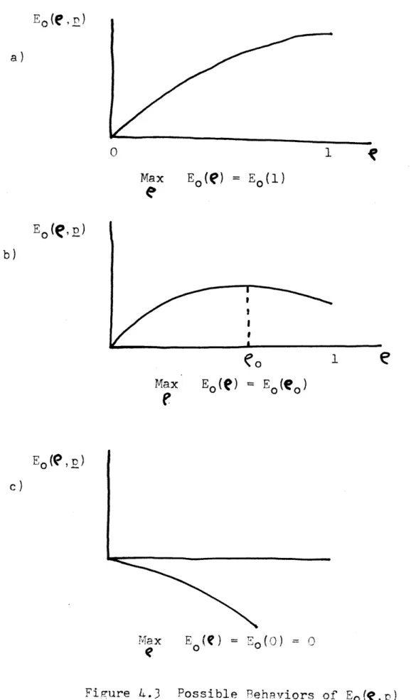
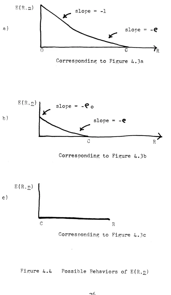
A Channel with Input Rotations 66 Possible Behaviors of Eo(e,2) 73 Possible Behaviors of E(R,n) 76

Chapter I Introduction

Most of the results pertaining to the reliability which may be achieved when data are transmitted over a channel have been obtained for the special case of the Discrete Memoryless Channel (DMC). Recent work of Fano , Gallager8_{, and Shannon, Gallager and}

Berlekampl9 has led to an almost complete specifi-cation of the smallest nrobability of error obtainable with maximum likelihood decoding of block codes for the DMC.

Collaterally, the investigation of practical

decoding techniques for the DMC has led to the design, construction and testing2 2_,2 3 _{of a sequential decoder}

based on the sequential decoding technique of Wozen-craft2 1. More recently, Fano5 _{has presented a new}

sequential decoder which appears to have great genera-lity of application.

Our nurpose in this thesis is to examine decoding techniques for channels that are not of the Discrete Memoryless variety. The channels with which we are concerned are such that at each discrete instant of time one of a finite set of symbols may be transmitted. One of a finite set of output symbols will then be received. The probability that a particular symbol

is received when a particular symbol is transmitted is a function whose value is determined by an

under-lying finite state stochastic process which is inde-nendent of the transmitted symbols. The aspect of memory is introduced by requiring that the proba-bility that the underlying process is in a particular

state at a given time is dependent on the sequence of states which the process has occupied in the past. In narticular, we will restrict this dependence to be Markovian, which (since we are concerned with

finite state processes) is equivalent to allowing the denendence to be over any finite span of previous states: A more careful description of the Channels is presented in Chapter II where appropriate notation is introduced.

A discussion of the broadness of the above model and some of its implications is also presented in Chanter II. We shall call this class of channels, Discrete Finite State Channels (DFSC); sequences of states of the underlying process will be called

channel state sequences.

In the following chapters we will examine both block and sequential decoding for the DFSC. The

denarture in philosophy taken here is that we attempt to decode by nrobabilistically testing both the

transmitted message and the channel states, rather than the transmitted message alone. Our primary interest is, of course, in the correctness of our decisions on the transmitted messages. The method of testing the compound hypotheses (both message and channel state), however, appears to be natural for sequential decoding. The reason for this state-ment lies in the fact that the joint statistics

of the output, and channel state, given a particular input, are Markovian, while the statistics of the output, alone, are not. By testing both the trans-mitted message and the channel state we are able to design a sequential decoder which operates in a step-by-step fashion closely related to the operation of such decoders for the DMC. Our ability to achieve such a design is a consequence of the Markovian statistics of the joint event (output and channel state).

A thorough discussion of the particulars of our decoding philosophy is presented in the next

chanter. We also discuss, briefly, several alter-native approaches to decoding which are suggested by the fact that the DFSC might be described as a time-varying channel. These alternative approaches are those that have arisen when, in engineering

Dractice, one considers what might be done to improve communication capability of such channels.

To operate in accordance- with the above philo-soprhy we must assume that the transmitter and decoder have an exrlicit probabilistic description of the

underlying process. This assumption may be questioned. We observe that this assumption is no worse than the assumption that the probability structure of a given memoryless channel is known. Experience in simula-tion of the DMC has shown that if the true probabil-istic structure of the channel is at all like the assumed structure, then the decoding will behave essentially as predicted theoretically (c.f,

Hor-11

stein ). We should expect the same to be true in the case at hand. In addition, knowledge of the behavior of decoding when the probabilistic

descrip-tion of the channel is known makes available a bound

to what might be achieved in oractice.

The DFSC fits within the class of channels for which Blackwell, et. al.1 have investigated capacity. In addition, Kennedyl3 has presented upper and lower bounds to the probability of error achievable with block coding for binary input, binary output DFSC's. Aside from these results and the previously referenced discussions of the DMC, no previous work of relevance to the DFSC appears to be in the literature:

In Chapter II we present a mathematical description of the DFSC and discuss the problem of decoding for

this class of channels.

In Chapter III we present various mathematical results which will be applied in the sequel.

In Chapter IV we find an upper bound to the probability of error which can be achieved by block coding for the DFSC when the method of simultaneously testing transmitted information and channel states is employed. A bound which decays exponentially with

the block length is found and compared to known results for the DMC.

In Chapter V we examine the behavior of the Fano sequential decoder when used on a DFSC. The results obtained here on maximum information rate for which the first moment of computation is bounded and for various probabilities of error and failure may be snecialized to the DMC. Certain of these results for the DMC were previously found by Fano . Certain

others have been obtained independently by Stiglitz (unrublished). The results for the DFSC have not been previously obtained.

In Chapter VI we summarize the thesis and suggest and discuss various possible extensions.

Most of the mathematical expressions, equations, and inequalities are numbered in succession in each chanter. For convenience, we will refer to all such exoressions as equations. When referencing a previous equation in the same chapter we give its number.

When referencing such an equation in a previous

chanter we give both the chapter number and the number of the equation. Thus for example, if in Chapter III we wish to refer to equation 2 of that chapter, we call it Equation (2). If, on the other hand, we wish to refer to equation 4 of Chapter II, we call it

Equation (2.4).

Chapter II

Introduction to Decoding for the DFSC

A. Description of Channels

We will be concerned with a class of channels where at each discrete instant of time one of a set of

K inputs, x4X, (x=1l,2,...,K) may be transmitted and one of a set of L outputs yCY, (y=l,2,...,L) will be received. The probability that output y is received when input x is transmitted is determined as follows:

Suppose we have a B state Markov chain with states dtD, (d=1,2,...,B) and a stationary (i.e.,

time-invarient) probability matrix

Q

=

(qij

)

where

qi j(i,j = 1,2,...,B) is the probability that when the chain is in state i, the next transition will be to state j. In addition, let there be a set of B2

probability functions, p(y/x,d',d) defined for all y _{Y, xgX and d',d D with the property that:}

p(y/x,d',d) _C

0

; all y,x,d',d ( 1)

and

I

p(y/x,d',d)

= 1

;

all x,d',d

(2)

Y

Suppose now that at some time the Markov chain is in state d' and a transition is made to state d, then conditional on this event, the probability that y is received when x is transmitted is p(y/x,d',d). Thus

trans-ition probability function for a fixed channel.

The aggregate of the Markov chain and the set of functions p(y/x d' d) will be called a Discrete

Finite State Channel (DFSC). We will call the

functions p(y/x,d',d) transmission probability func-tions, and sequences of states from the Markov chain

will be called channel state sequences. In this

thesis we will restrict ourselves to the case in which the underlying process (i.e., the Markov chain) is irreducible.

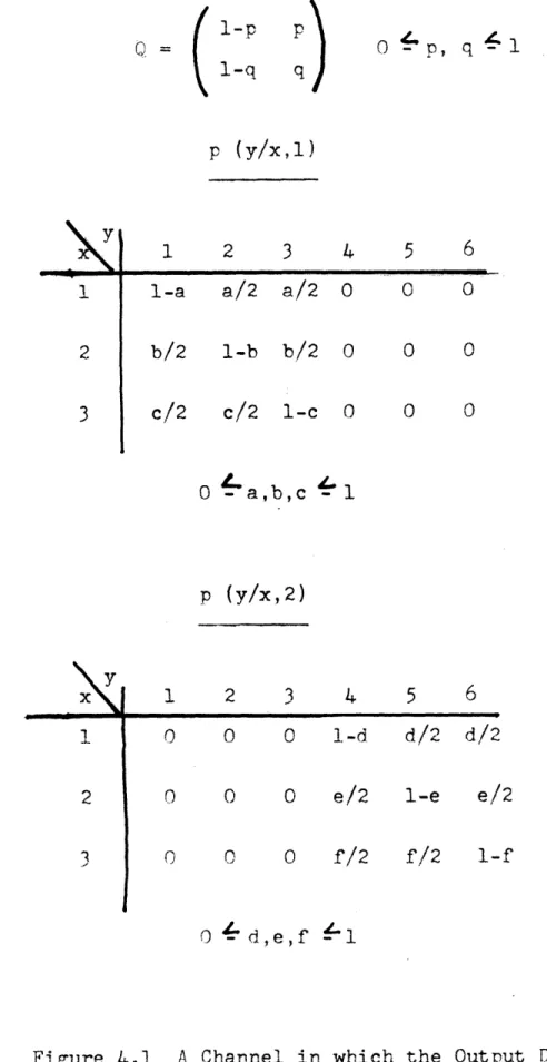
Let us pause for a moment and consider the generality of this definition. Although we have defined the transmission probability functions

o(y/x,d',d) on the state transitions, we have

clearly included the case in which it is desirable to define these functions on the states. To

demon-strate this inclusion we need only observe that if we allow p(y/x,d',d) to be independent of d' (or d) our functions are then defined on the states.

Another model which might be considered is the following: Let there be a set of A probability

functions p(y/x,c) ; (c=1l,2,...,A). These functions determine the probability of receiving a given out-put when a given inout-put is transmitted, for the event c occurring. Further, let there be a set of B2

H (c) 0 ; H-- Hd (c) = 1 (3)

d',d c=l d',d

where Hd ,d(c) is the probability that, when a

transi-tion of the Markov chain from state d' to state d takes place, the transmission probability function which determines the input-output statistics is

p(y/x,c). The resulting situation may be modelled as a DFSC in either of two ways.

First, each state, d, of the chain may be split into A states, dl,d2,..., dA one for each value of c.

For the resulting model we then have:

Pr (d _{/ d'c,)= Hd',d(c) qd',d (4)}

and

p(y/x,d' c,d )

=

p(y/x,c)

(5)

A second alternative is to retain the original description of the chain and take:

A

p(y/x,d',d)

=

21.

p(y/x,c) H d(c)6)

C=I

where we observe that the above equation defines a valid transmission probability function.

We shall find that because of the decoders em-ployed for the DFSC as discusssed in later sections of the chapter, and because of the techniques used to

bound the behavior of these decoders, it is generally desirable to model the channel with as small a number of states in the underlying Markov chain as is possi-ble. For this reason, the second alternative discussed above is adopted when we have such a choice available.

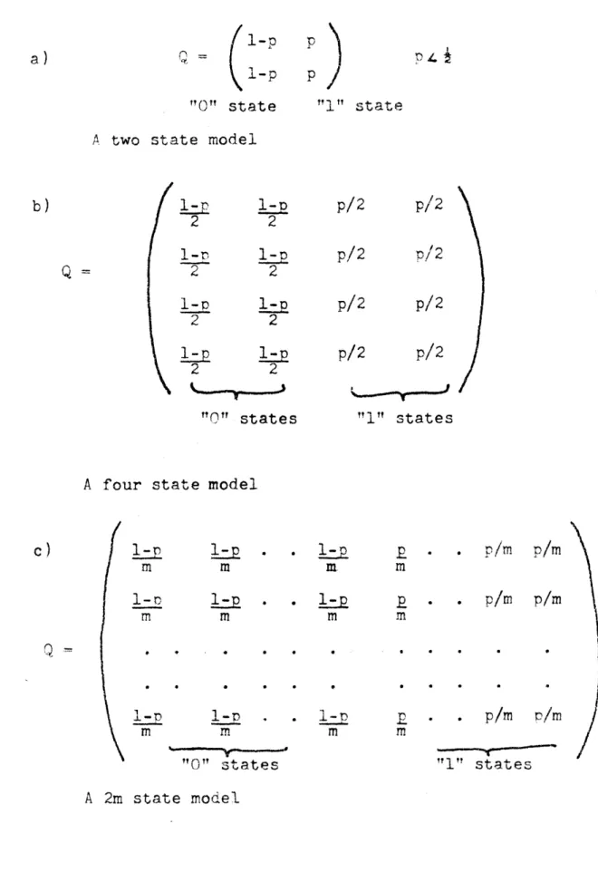
To illustrate further the multiplicity of models which may be used to model a DFSC we consider the

special example of a memoryless Binary Symmetric Channel. We may, of course, use the one-state model of the channel as is the usual choice. (Note here that a memoryless channel may always be taken as a DFSC with a single state in the underlying Markov

chain). We may also choose a model in which we

associate the transmission probability functions with states. We distinguish two types of states, 'a 0 state and a 1 state with transmission probability functions as shown in Figure 2.1. We may then take any of the models shown in Figure 2.2. Each model clearly is equivalent to a BSC with cross-over proba-bility p. This particular example is of great inter-est since it allows us to discuss certain deficiencies of our decoders. We will return to this matter in Chapter IV.

To denote sequences of random variables we will use the symbol for the random variable underlined

p(y/x) for a "0" state

x

1 2

1 2

p(y/x) for a "1i" state

f

-1 2

±

Figure 2.1 Transmission Probability Functions for "0" States and "1" States

16

Q

l1-p

1-p

"O0" state

P

"i" state

A two state model

2 1-D 2 12

2

2 2 2 2

p/2

p/2

p/2

p/2

"O" states

"1" states

A four state model

1-p l-p

m

1-p rn "0" states

l-p

Z.

m rn 19 m *

. p/m p/n

. . p/m p/m "1" states A 2m state model

Figure 2.2 Alternate Models for a BSC

17 p/2 p/2

p/2

I

I

1-n rn I-_m

&-a &&-amp;

of elements in the sequence. Thus a sequence of n channel inputs will be denoted by x(n). The set of all such sequences, which is the n-fold cartesian

product of the set of all values of the basic one-dimensional random variable will be denoted by a

superscript on the symbol for the one-dimensional set. Thus we speak of x(n) Xn. The position of a particular element of a sequence will be denoted by a subscript. Then, making the obvious analogy of sequences to vectors and elements to components of the vector, we write:

x(n) = (x1,x2,...,x_{n )} (7)

One exception to this rule is that for channel state sequences we will speak of d(n)6 Dn,

d(n) = _(do,dl,...,d

n ) 8)

which is actually in Dn+ l_{. The reason for this}

convention is the simplification of notation and this convention should be remembered since it is in continuous use in the sequel. The inclusion of d specifies the initial state. As an additional notational convenience we introduce the symbol di,

d

=

(d. ,d) ₍₉₎

1 i-l,

The notation of equation (7) suggests that we interpret x(n) as a row vector. We will use an overbar to denote matrix transposition. Thus x(n) is a column vector.

The standard introductory reference on Markov chains is Feller7. The algebraic treatment of Markov chains in terms of Frobenius's theory of matrices with non-negative elements is given in detail in Gantmacher9. An excellent discussion incorporating aspects of both Feller's and

17 Gantmacher's treatments is given by Rosenblattl7

B. Block Decoding for the DFSC

We now begin our study of decoding for the DFSC. The situation of block coding is dealt with initially because it is inherently simpler to discuss than

sequential decoding.

nR

We wish to transmit one of M = e equally likely messages over a DFSC. To do so, we select

a set of M channel input sequences x (n); m=l,2,...,M, and transmit sequence x (n) to signify that message_-Tn m occurred at the transmitter.

Upon receipt of the output sequence Y(n), we attempt to guess which message was transmitted. The best guess, in the sense that it would minimize our orobability of error, would be that given by a maxi-mum likelihood decoding scheme. In this case we

decide that message k was transmitted if

Pr(y(n) / x (n) ) max Pr(Y(n) /x (n) ) (10)

The probability of error for such a decoding scheme is not readily analyzed for the DFSC, but in principle we may always perform maximum likelihood

decoding. The result we expect to obtain when properly chosen block codes are employed on the DFSC is that for rates, R, less than some yet to be determined canacity we are able, by increasing n, the block length, to make the achievable error probability arbitrarily small.

The difficulty that arises, when we attempt to analyze block coding bounds on error probability for maximum likelihood decoding, is that an early step in our derivation of a bound reduces the sharpness of the bound to the point that it is equivalent to a bound on the behavior of the non-maximum likelihood decoder which we ultimately study..

How does one decode for the DFSC? Experience with time-varying channels in general has led

various investigators to suggest schemes based on heuristic reasoning. One such scheme may be described as follows: _{From the received data make an estimate} of the channel state sequence. Then, assuming that this estimate is correct, do maximum likelihood decoding as if this assumption were correct. This scheme is embodied physically in such systems as Rakel4 and in systems which utilize techniques of phase estimation and coherent demodulation with the

estimated phase for channels with a time-varying rhase shift. This latter scheme is analyzed in some detail by Van Trees23. Although these examples

apply to continuous channels, the philosophy of anproach is clearly applicable to the case of the DFSC. The aspect of these schemes which make them attractive is that for the particular situation for which they are intended, they are readily instrumented

in practice while maximum likelihood techniques are not. Both schemes show the following deficiency:

The estimate of the channel state is made independent-ly of any hypothesis on the transmitted information. This factor may or may not be bad. Whether it is or not depends on the complex of the rate of transmission, the nature of the particular channel at hand, the

choice of modulation, and the interactions among these.

Now consider how such schemes may be applied to the DFSC. We have some rational for deciding that a oarticular channel state sequence d*(n) has occurred. Then, assuming this decision is correct, we compute: Pr(y(n) /x (n),dj(n) ) for each k = 1,2,...,M. We then decide that message m was transmitted if:

Pr(y(n) /x (n),d*(n) ) = max Pr(y_(n)/x (n),dI(n))

_"m

(11)

-k

The behavior of such a decoder clearly depends on the method of choosing d*(n). Such methods arise from what amounts to good intuition applied to the

parti-cular case at hand. Since we are interested in a broad class of situations, it is unlikely that such intuition could be applied in general. A way out is described below.

Suppose we broaden our approach to include joint estimation of both the channel state sequence which occurs and the transmitted message. We are then not forcing ourselves to decide on the channel

state sequence first. Of course, as in the examples discussed above, our primary interest lies in making our decisions on the transmitted message correct. The

penalty we pay for being wrong on the channel state sequence is zero if we are right on the transmitted message.

This concept of joint estimation arises in an internretation of the maximum likelihood recievers for gaussian signals in gaussian noise (see Kailath1 2

20

and Turin _). In this case the receivers may be

realized in a form in which an estimate is made of

the shape of the gaussian signal conditional on the transmitted message having been a particular one. This estimated shape is then used as a reference for a correlation receiver for that particular message. One such estimate and correlation operation is

per-formed for each different transmitted message hypothesis. 22

A class of decoders may now be thought of immediately. We may for example consider the function Pr(y(n)/x (n),d(n) ) for all values of both d(n) and k. The decoding rule could then be: _{choose message m as transmitted if}

max Pr(y(n)/x (n),d(n)) = max max Pr(y(n)/x (n),d(n))

d(n) _{k d(n)k}

(12)

An objection to this decoder which might be raised is that for a particular message which is not the transmitted message, there might be a particular channel state sequence d*(n) such that Pr(y(n)/x(n),d*(n) ₎ is very large.

There are at least two ways of avoiding this unhappy situation. First, by appropriate choice of modulation (i.e., the choice of the x (n)'s) we

-k

might be able to avoid the possibility of this occur-rence. Again, such a choice is to be found by

applying good intuition to the particular case at hand.

A second alternative lies in weighting the probabilities in Equation (12) by a factor which takes into account how probable any sequence d(n) is a priori. We may, for example, take a binary weight and assign weight 1 to those channel state

sequences whose probability exceeds a given thresh-old, (say n ) and weight 0 to the remainder.

Thus if we let D be a set such that: 0

Do ={d(n) Pr(d(n)

po

0

(13)

o c

and let D_o be the complement of this set we might formulate a decoding rule as follows: Pick message m as transmitted if:

max Pr(X(n)/x (n),d(n) )

d(n)eD m

i-

o

max max

Pr(y(n)/x (n),d(n)

)

(14)

k d(n)ED

-k

f o

An upper bound on the probability of error for such a decoder can be found, but it is not presented here because it is weaker than the bound for the decoder we do analyze.

The idea of weighting the probabilities in Equation (14) can be extended to the logical conclu-sion of using as weights the actual a priori proba-bilities of the state sequences. Thus we are led to the decoder to be employed in this thesis. Our de-coding rule is stated as follows:

Choose message m as transmitted if:

max Pr(v(n)/x (n),d(n) ) Pr(d(n) )

d(n)

m

= max max Pr(y(n)/x (n),d(n) ) Pr(d(n) ) (15)

k d(n)

--24

Now, we note that:

Pr(y(n)/x (n) ) Pr(y(n)/x (n),d(n)) Pr(d(n) ) (16)

D m

It would seem reasonable that, if Equation (15) is true, then with high probability Equation (10) is true. We have not proved the above statement, we have merely suggested its validity. The true rela-tionship between a maximum likelihood decoder and the decoder to be used in this thesis is explored further in Chapter IV.

It is clear that to evaluate the max's in

SEuation

(15) the decoder must test every channel

state sequence. This concept of testing both channel state sequences and transmitted messages in order to decode leads to the title of this thesis, "Channel State Testing in Information Decoding". In our decoder we are, in effect, deciding on both the transmitted message and the sequence of channel states. Although we make the latter decision, our primary interest is in the transmitted message and hence in Chapter IV we shall evaluate an upper bound on the probability of decoding error without regard to the probability that the decision on the channel

state sequence is correct.

This decoder has the advantages that we are able to obtain an analytical bound on its error probability.

i25

Furthermore, this bound has the desired property (an exponential decay with n) that we would hope to find. Still further, the decoder metric (i.e., Pr(y(n)/xk(n),d(n)) Pr(d(n)) may be, with slight

- - -- - -- - _ I__L -

-modification, usea as a metric (see thne next section) for a sequential decoder.

That these advantages are obtained should not be construed as meaning that the other decoders discussed above or, in fact, any decoder based on good heuristic reasoning should be precluded. We shall find, for example, that there are many situa-tions in which our decoder is a poor choice. This may be due to the fact that the model chosen for a particular channel is a poor model or that the decoder itself is inherently poor for the case at hand. We can better discuss such matters in Chapter IV.

The point to be emphasized here is that for our -I •1~J F• I A .• ~ • • I

•

-2 • I -I...

--- tI- •

C C I'~ UI IC) I-' U WI"' (~-~ t'1 ti Cii .-4 I TI -I rIrIllV'C(1 r~TI ~7T'fT ~ 7'i!~ ~v, I ~ 'I" ¶?

whose strengths and weakness in any particular case orovide an opportunity to examine the issues at the heart of decoding for the DFSC. In the almost total absence of prior results for channels which are not of the discrete memoryless variety, this opportunity was not previously available.

26

C. Sequential Decoding for the DFSC

In block decoding we face a dilemma. As we increase n to make the error probability arbitrarily small, while holding the rate, R, constant, the number of messages M = en R grows exponentially, since for the various alternatives of block decoding discussed above, we must test each possible transmitted sequence. Thus we will, in general, face an exponential amount of computation.

These remarks apply to the DMC as well as the DFSC. In the latter case, for our decoder, the situa-tion is even worse. We must also test every possible channel state sequence. The number of these also grows exponentially with the length, n, of the code.

The most successful technique for avoiding this exponential amount of computation has, in the case of the DMC, been the sequential decoding technique of Wozencraft2 1. Recently, _Fano5 has presented a new

sequential decoding algorithm which appears to be somewhat more general. We will use the Fano algorithm with a slight modification to do sequential decoding for the DFSC.

We will restrict the underlying process to

i

h ave the property that each state may be reached from each other state in a one step transition.

27

The reason for this restriction will be explained in Chapter V where we discuss its implications.

We assume that the information to be transmitted arrives at the encoder as a stream of equiprobable binary digits which we will call information digits. The encoder is considered to be a finite state device to which are fed

Volog

2e information digits at a time

and whose state at any given time depends on the last

V

log2 e information digits which it has accepted. The

state may also depend on a particular function of time selected by the designer of the encoder. The encoder output at a given time is then determined uniquely by its state at that time and hence depends on the last V log 2e information digits fed to it.

Such dependence is most readily represented as a tree code in which a particular set of information digits trace a path in the tree along which are listed the

channel input symbols generated by the encoder (see Figure 2.3).

The leftmost node of the tree corresponds to the initial state of the encoder which can be assumed to be a state corresoonding to a stream of all 0 information digits having been previously fed to the encoder.

Each branch corresponds to a particular state of the encoder which is specified by the order number of the branch (i.e., how far into the tree the branch lies) and the last

V

log2e information digits leading to it.

n

O M =M r-0 0 0

I

r- Hi *1 IH f-i H 0l H-29 0 H? 0 r-0 C3 r- 0 H r r U-0 II 0) Hr 41l U) (Ni · ci 0 U) C) H-0 H-1 r- o H-0 I I ) q H I 6wý M-C)II r-t I C I C r-cj i i l i

I

V

N = olog2e

(17)

for each branch.

Now consider two different paths stemming from the same node of the tree. Call this node the

reference node. Because the state of the encoder depends on the lastV log e information digits fed

2

to it, these two paths must correspond to a sequence of encoder states which are different for at least

/•0 branches. Beyond this point corresponding states along the two paths will coincide wherever the sequences of the last V10og 2e information digits

along the oaths are identical. Two paths stemming from a reference node are called "totally distinct" if the sequences of encoder states along them differ everywhere beyond (i.e., to the right of) the refer-ence node.

30

L

In the figure the information digits are shown just to the left of the branch they generate. The channel symbols corresponding to each branch are shown just above the branch in question.

We assume that the rate, R, is measured in natural units per channel symbol. Thus the number of channel symbols per branch, N is given by:₀

The above description of tree codes has been

6

paraphrased from Fano . In Chapter V we will be concerned with an ensemble of such codes. Let us observe at this point that the ensemble (and certainly every member of it) can be generated by an appropriate ensemble of linear feedback shiftregister generators to which are added devices containing stored digits to establish a particular encoder. We will not dwell on the realization of these encoders here, since they

16 have been adequately discussed by Reiffen and

5,6

Fano ; but we do state the result that the encoder need have a complexity, as measured in terms of num-ber of elements, that grows only linearly with .

Note thatylog2e in this case corresponds to n, the block length, in the case of block coding.

Let us now discuss the method of decoding to be

A Tl P il 1 1- h h

LILL UP:e e sU111 0 am 1a .

iarit

Y

i tý eU ao decoder for the DMC. The decoder computes a metric depending on received and hypothesized transmitted

s.mbols for each branch along a path which is being tested. The running sum of this metric along a path

under test is computed. The metric is so chosen that for the actually transmitted path this sum has, with

hi

roabiit

A monotnen

inc-reasing- (wit-.h

ript11

into the tree) lower bound. The decoder is so

de-signed that it searches for and accepts any path having

I1

which are consistent with the state sequence accepted to this node. This concept of jointly testing both message and channel state sequence hypotheses, follows from the discussion of the preceeding section of this

32

this property. More precisely, if there are more than one path which have this property, the decoder follows one of them. The decoding procedure is a step-by-step procedure in which each branch is tested individually (rather than long sequences being tested at once as in block decoding). The deoendence with depth into the tree arises from the fact that the branches which may be tested at a given time are restricted to those stemming from a tree node which lies along the path accepted up to that time. This reference node is continually up-dated as the decoding proceeds further and further into the tree. The meaning of this description will become more clear when we examine the details of the decoder for the DFSC.

To adapt the Fano decoder for use on the DFSC we will construct a metric for that case. The view-noint that we adopt is that we attempt to decode the compound event of transmitted message and channel state sequence which has occurred. Thus, having accented a path in the tree up to a certain node, the decoder tests all branches stemming from this node, and simultaneously all channel state sequences

chanter.

Let us now be more precise. Define an arbitrary orobability distribution f(y) on the channel output symbols, such that:

f(y))O _; y=1,2,...,L L

. f(y) =L

y=1

(18)

Now for the branch of order number n, with a particu-lar hypothesis on the transmitted symbols and a

particular hypothesis on the channel state sequence, consider the metric

nNnN₀ o(yv/xj,d )qd ->d _j-1 In - U n j=(n-l)N y+1 f(Yj)

(19)

where U is an arbitrary bias.

This metric is the extension to the sequential decoding case of the metric used in the previous section. The significant difference lies in the inclusion of f(y). This function plays the same role here the p(y) plays for the Fano decoder for the DMC. Ideally we would like to include a state

derendent term in the denominator of the argument of the logarithm in Equation (19). We do not do so

because we have found such a term to be analytically intractable. The price we pay is that our results for sequential decoding for the DFSC will not, in all

cases, bear the same relationship to the results for block coding that is borne in the case of the DMC.

Note that the metric requires knowledge of the present output symbols; the present input symbol

hypothesis along the path being followed, the present channel state sequence hypothesis and the most recent channel state hypothesis. Thus, the metric can be computed for each branch in a step-by-step manner which requires only the presence of a tree code

generator and a minimal storage of the previous state decision at the decoder.

Now for a particular path in the tree code and a narticular sequence of channel states assumed in the decoding define:

n-l

L _{= .} .

n j=l J ₍₂₀₎

The decoder to be presented below attempts to find a path in the tree and a corresponding sequence of channel states such that along this oath the

sequence of values L has a monotone increasing lower bound.

The operation of the decoder is best explained by examination of a flow chart for it. In Figure 2.4 we present the flow chart.

Here we assume that at each node the branches are numbered in order of the value of the metric along them. Thus gl(n) is the largest value of the metric (consistent with the state assumption on the

Previous symbol), and j(n) = 1,2,...,P e' °

Define g. = _{max gi(d)}

1 d , i d

(21)

Here d is a particular channel state assumption associated with the branch in question. We assume the branches are numbered in order of the value of p and g l(n)is the largest value of the metric

consistent with the state assumption on the previous symbol and i(n) = 1,2,...,eVo

Finally,

1 - F stands for: set F equal to 1

Ln i(n± L set Ln+1 equal to L +i(n)

n _{j (n) Ln+l} n 4 1 n-4"n i(n) •i-i (n) T To--pT n+1 T " " " " " L +g.(n _j(n)

"! " substitute n+l for n (increase n by one)

" " substitute i(n)-~ for i(n) " " _{substitute T + To for T}

Scompare L and T; follow path marked 4 if Ln+1I T.

U0 OO0 OO

7

The operation of the decoder is essentially the same as the operation of Fano's decoder in the case of the DMC. The difference lies in the fact that when the decoder is moving forward (i.e., following a path for which L is continually increasing) the

n

only state hypotheses utilized are those that maxi-mize the metric for each particular message hypothesis. When the decoder is moving backwards (i.e., following loop B or loop C) for the first time however, we

allow the state assumptions to vary over all states consistent with the state decision on the branch preceeding (in order of depth into the tree) the branch presently under investigation. We need never allow this variation for more than one step backwards. This follows from the fact that with Markovian

statistics the state sequence can always be forced into any desired state in a one step transition

(under the present hypothesis that all states are reachable from all other states in a one step transi-tion). Thus, if a particular path in the tree with a particular channel state sequence hypothesis is one that the decoder can follow successfully, we can always move from this same path with a different state

sequence hypothesis to the desired one in a one step transition.

The flow chart presents an equipment whose com-plexity is independent of

V.

It is intuitively clear that as the parameter)increases the required speed

thus evaluate an upper bound on a quantity relating to this required speed in Chapter V under the

assumption that = 00 .

The quantity which is bounded is the average number of times the decoder follows loop A per node decoded. What we mean by "per node decoded" is the

following: We shall find (see the next few para-graphs) that the decoder follows a path which agrees with the transmitted path almost everywhere with over-whelming probability. To ultimately follow this path the decoder may examine a given branch more than

once (by being forced back through loop B or C). Once the decoder has examined a given branch on the ultimately accepted path for the last time, we may

say that the node(i.e., the information symbols)

preceeding this branch has been decoded. It is intuitively clear that most of the time the decoder will follow loop A if it is to ultimately get anywhere.

Thus the bound on the average number of times loop A is followed per node decoded gives a reasonable measure of the speed with which the decoder must ooerate. _{The result obtained in Chaoter V is that} for rates of information transmission smaller than a rate R , this number of traversals of loop A

(i.e., the number of computations) is bounded while for rates exceeding R it is not.

An investigation of the decoding algorithm leads to the conclusion that the decoder never makes an

irrevocable decision. This follows from the fact that the decoder may move backwards in the tree

(i.e., to the left) by following loops B or C. There is no limit to how far back the decoder may move. We may obtain an appreciation for the proba-bility that the decoder ultimately follows the correct

path, by inhibiting the ability of the decoder to move backwards indefinitely. If we constrain the backward motion to a fixed number of nodes, which we call a constraint length, we can then determine the proba-bility that the decoder has made an incorrect decision at any node once it moves a constraint length ahead of this node. It is this event which precludes the nossibility of the decoder ever moving back to change its incorrect hypothesis. This probability is

upper bounded (as in the probability that the decoder is ever required by the algorithm to move back more than a constraint length) under the assumption that

c)

= co. The reason for this assumption will become clear in the next paragraph. It is found that both of these Drobabilities decay exponentially with the

constraint length for rates smaller than

R Thus

Scomp

if the rate of information transmission is smaller than _{R we are assured that, except for the errors}

to be discussed in the next paragraph, the decoder will eventually follow the correct path if the

con-straint length is infinite.

There is a class of errors which the decoder can make which we call undetectable errors. These arise in the following fashion. Suppose the decoder follows a path which is correct to a given node, but then is incorrect for the next, say, k information digits, and then is correct once more for the informa-tion digits beyond this point. Because of the method of encoding the correct path will differ from this

k

oath in k + i)-) o ) log2e branches, but will

Slog2e 0 2

agree everywhere else. If the metric on the correct oath has a monotone increasing lower bound, then so does this particular incorrect path since the two

agree in all but a finite number of branches. Thus

4h n it 4 ci ed csa Le- +i v h the d

may follow this particular incorrect path and yet never detect that such an event has occurred. The results quoted in the previous paragraph establish that with orobability one, the decoder will detect an error that occurs from its following a path which

is totally distinct from the correct path beyond a given node. Undetectable errors arise only on paths which are not totally distinct from the correct path.

"II

41

L4

In Chapter V we will find an upper bound on the average number of undetectable errors made per node decoded. It will be found that this bound decays exnonentially with 'V and hence all errors may be reduced in probability to arbitrarily small values by increasing 9 .

The probability that the ultimately accepted channel state sequence is correct is ignored. We in effect consider all errors in the channel state sequence to be undetectable. It is for this reason that we allow the decoder to change state hypotheses

only one step into the past. We justify our viewpoint by observing once more that if the decoder follows the nath corresponding to the transmitted information digits, then errors in the channel state sequence are of zero cost.

*1

(Ii

)(

b 1-A

(1-A)

b

- (

a

bi

)

i=1 i i=1 i=1

(3)

42

I

Chapter III Mathematical Preliminaries

We interrupt the flow of the thesis at this point to introduce some mathematical results which are required for the following chapters.

A. Convexity and Some Standard Inequalities We list here some standard inequalities which will prove of use in the sequel. Proofs and

discus-sion of these inequalities may be found in Hardy, 10

et.al. . Throughout, we take A to be a real number

with

0

o•

•

(1)

The Inequality of the Algebraic and Geometric Means:

Let a,b O0. Then

x (l-A)

a b +Aa + (1- X)b (2)

Holder's Inequality:

Suppose a.,b- Ž0 ; i=1,2,...,N

Then

r

Two additional inequalities of interest are: N i=1 i and. if L- b = i=l i (i.e., b ij is N

•

ba

X i=l 1 i

a probability distribution) then

N

_ (i

b.a )

(

i=l I1 (I

6)

Minkowski's Inequality:

Suppose a. i 0; i=l,2,...,N ; j=1,2,...,M. Then

N M 1 M 2 ( ai ): i=1 j=1

j=1=

N

(

a

i

)

i=l

(7)

We next quote a few results on convexity. A good discussion of these results is given in Blackwell and Girschick2

A set, C, of elements c is said to be a convex set if for every c,c'EC and every

Xsatisfying

equation (1) we have:

Ac

+ (1-A)c'

C

)

a. 1 (4)

(5)

4

z

(8)

1

eorem : necess

d

tion that r* minimize F(p) is that: there exists a real number,A, such that:

44

I:~

The elements may be vectors.

A function, F(c) is said to be convex over the set, C, if

F(Ac

+

(1-A )c')

AF(c) + (1-A) F(c')

(9)

If the inequality is reversed the function is said to be concave.

A sufficient condition for convexity of F(c) where c is a real number in some interval and F is twice differentiable is that:

2

d22 F(c) - 0 (10)

de

This condition is also necessary if F is differentiable, but a non-differentiable function may be convex.

Clearly the set of n-dimensional probability vectors

S= (plP2"",p_)n

M

P. ; = (11)

1 i=l i

is a convex set. In this event we have the following snecial case of the Theorem of Kuhn and Tuckerl .

_

F(p)

- A

;

p > 0

(12)

and

P I p = - - A; p = 0

(13)

Equation (13) allows us to determine if in fact the minimum occurs on the boundary of the set of probability vectors (i.e., for some components of the vector being equal to zero).

B. Bounds on Functions over a Markov Chain

In this section we discuss bounds for functions defined over a finite state Markov chain. The basic results stem from Frobenius's theory of non-negative square matrices (see Gantmacher9_{). The essentials}

of this theory are given below as Theorem 2.1, We begin with a discussion of irreducible non-negative matrices.

A B x B matrix Z = (zij) is non-negative (i.e., Z - 0) if

Z O0 for i,j = 1,2,...,B (14)

The matrix Z is said to be irreducible if it is impossible by a simultaneous permutation of rows and columns of Z to put it in the form:

Z , O

Z _z3 0Z

z 2

where Z and Z are square matrices. Clearly the

1 2

probability matrix of an irreducible Markov chain is an irreducible matrix.

A vector v = (v ll12,...,v ) is said to be

greater than a vector v2 (v21,v 2 2,...,V 2B)

(i.e., v1 v2 ) if Vlj v j 2 ; j=1,2,...,B (15)

Frobenius's theorem then states: Theorem 3.2:

An irreducible non-negative matrix, Z, has a largest positive eigenvalue u which has the following properties:

1) u is a simple root (i.e., of multiplicity one) of the characteristic equation

Z - uI

= 0

(16)

2) If w is any eigenvalue of Z then

W

I

u

(17)

3) There exist positive left and right eigen-vectors v and x of Z with eigenvalue u

i.e., Z x = ux ; x>,0

Y Z = uy ;

V

>0 (18)

1

z(Xt

₁

-

(1- )t ) _Z(tl

₂

₁

)

z(t )

₂

SXz•(t

) +

(l-A) z(t

)

(22)

1 2

The first inequality above comes from the logarithmic convexity. The second inequality comes from the

inequality between algebraic and geometric means (Equation (2 ) ).

47

r

4) If w is a positive eigenvector of Z then w has eigenvalue u.

5) Let )> 0 and w> 0 satisfy the equation

Z 7 !.A w (19)

,

then A uu

where the inequality is strict unless w is an eigen-vector of Z.

6) u is a monotone function of the matrix elements. That is, if any matrix element is increased, then u

is increased.

In the sequel we will be interested in exponen-tial bounds for the powers of the matrix Z (t) where

Z (t) = (z.ij(t) ) (21)

and each z..(t) is positive, twice differentiable, 1j

and logarithmically convex in some range of real t, to t t t . We say a function, z(t) is logari-thmically convex if ln z(t) is convex. This implies that z(t) is convex since for 0 -

X

) 1

Now let the nth power of Z (t) be

S (t = (z (t) ) (23)

then we have the following theorem: Theorem 3.3:

Let Z (t) be a B x B non-negative irreducible matrix with elements z. (t). The elements,

(n)(t) f the nth Jl

z. (n)(t), of the nth power of Z (t) satisfy the inequality:

B

Al(t) (u(t) )n. z (n)(t) ý A (t) (u(t) )

j=1 ij 2

(24)

Here u(t) is the dominant eigenvalue of Z (t) and A (t) and A 2(t) are positive and independent of n. Furthermore, if the z. (t) are all twice

differ-Ij

entiable and logarithmically convex, in a region t - t 4t , then A (t) and A 2(t) are twice

differ-entiable and u(t) is twice differdiffer-entiable and logari-thmically convex in the region t 0 t 4 tl

Proof:

Let b(t) be a positive right eigenvector of Z (t). Then

B

T- _{z..(t) b.(t)= u(t) b (t) (25)}

and (n) (t)

_(t)

j=1

ij

Now since b(t) component b,(t) and n

(u(t)

)

b (t)

b (t)

(26)

is positive it has a smallest a largest component _b'(t).

Thus

(u(t) )n

S

1

b'(t) 1 b.*(t) b!(t) b*(t) Here A (t) and B

j='

(n) z (t) b ij j j (n)

(t)

(t) b (t) = J (u(t) ) = b*(t) b (t) A (t) = 2 b'(t) b*(t)

are positive and independent

Next observe that u(t) is a solution of the equation:

(t)

= 0 ₍₂₉₎ 49

b*(t)

b'(t)

(u(t) )

h (tI)

b'(t) (n) 1= -(t) b.(t) b*(t)

(u(t))

(27)

(28)

of n. v ! i=l i

The left hand side of this equation is a poly-nomial of degree P in v, each coefficient of which is a polynomial in the elements z..(t) of Z(t).

13

Since these elements are twice differentiable, it follows that u(t) is also.

Now since u(t) is a simple root of Equation (29) it follows that the matrix

Z(t) - Iu(t) = (zij(t) - i u(t) ) (30)

13

ij

has rank B-1. Furthermore, since the matrix Z(t) was irreducible, the vector a with components

I

a

= 1

₍₃₁₎

1

a. = 0 ; 1Zi

4

B (32)

must be linearly independent of the first row of Z(t) - iu(t). Thus the B x B matrix Y(t) formed by deleting the first row of Z(t) - Iu(t) and replacing it with a must be non-singular. Thus the equation

y(t)

E

(t) = (1,0,0,...,0) ₍₃₃₎ serves to specify b(t) which is independent of n. If all coefficients of the b (t)'s in the above

i

equations are twice differentiable, it follows that b (t)'s are also. Thus A (t) and A (t) must be

i 1 2

! twice differentiable.

Now let t s, r t . Then define the vector 0o

b with components:

b = (b.(s) )

i

1

(b.(r) )

1

for 0 4 X 4 _{i. Then we have}

-

(z s + (l-

)r) b

(1- X)

; i=1,2,...,B

(34)

j=1 ij

-

Z[

(s)

b

(s)

A

(r) b (r)

=

ij

j

ij

j

(

by virtue of the logarithmic convexity of the

z..'s.

13

Now arplying Holder's inequality

_{(Equation(3) ) we have}

A

z (Xs + (1-A)r) b

j=1

13

B

_B

1-Sz. (s) b (s)

z

(r) b.(r)

= ij3

13

3

&--u(s)

u(r)

(36)

Thus by Equation (20) of Theorem 2.2 we have:

)

)1-A

u(As

+

(l-A)r)4 (u(s)

(u(r) )

₍₃₇₎

35)

r·

Thus u(t) is logarithmically convex, if the z..(t)'s

ij

are. Q.E.D.

The above theorem is essentially the same as

13

that given by Kennedy . Our proof differs somewhat in detail and appears to be simpler. We now prove Theorem _3~4:

Let V(t) be a non-negative, irreducible matrix with elements

1

z..(t) t, where the z (t)'s are

13J ij

logarithmically convex in the region t t t .

o 1

Let v(t) be the dominant eigenvalue of V(t). Then t

(v(t) ) is logarithmically convex in the same region of t.

Proof: Let b(t) be a positive right eigenvector of XV(t) and let to 0 s,r tl. Then define the

vector b with. components

"s

•s+(l-4)r

b - (b

i

(s

)

)

for 0 X- 1. Then we have

B

Sz.

*(>s

+ (l-A)r)

j=1

B

_l S (

1

~Z

z. (S)

(b.(r)

₁

(l-

X)r

X s+(1-X)r

(38)

1

s + (l-A)r

As+(l-• )r

r

As+(1-)r

b.(s) _(rb

ij

i

(39) 52

by virtue of the logarithmic convexity of the z (t)'s.

i

j

Now applying Holder's inequality (Equation 3) we have:

L.

z.

(,s

j=1 13 £4

.

.(S)

AsT+(l-A)r

I

b.(s

F

j=l 11 r z (r) bi(r) ij (-1-X)r

xs+(l-A)r

-

(v(s) )

X s

As+(l-A)r

Thus by Equation (20) of Theorem 2.2 we have:

X

(l-)rA)

(v (s) '

Xs +(l-A)r v(r

) rJ As + (I-A1r

It follows then that

X s +(l-A)r (1-A)

-[(v(s) )s]

(v(r))r

(42)

Q.E.D.

We now prove the following corollary to Theorem 3.3.

(1-A)r

(s+(1-X)r

(v(r) )

(40)

v(As +(l-)r) 4

v(As +(1-A)r)

Corollary (3.1):

Let V(d(n) ) = g(d )

-0

_k=1

TT

v( )

_k

A

where v(dk ) is a non-negative function defined on the

state transitions of a Markov chain and g(d ) is a 0

non-negative function defined on the states. Then

(44) Ln

_D

V(d(n) ) -A^t

where/(A is the dominant eigenvalue of the matrix O = v(i,j)

and A is positive and independent of n. Proof:

Let

~n

=(v(n)(i,j))

Now by Theorem 2.3 we have:

B

i

Z

g(i)v(n)(i,j)

4 A

i=l j=l

where the constant, A, includes the factor

g,+i). Next observe that by the definition of matrix

multi-nlication

Z

d

=1

I k-I

v(d k_)

v (dk)

54

(43)

(45)

(46)

defines the element v( 2 ) ( d _{_}

, d ) of the matrix 2

(~dk-2 oftemtiJ

Thus, upon itterating the sum on Dn in Equation (44) and performing the innermost n-1 sums, we recognize the identity

B B

V(d(n)

)

I X

g(i)

v (i,j)

(47)

n

D i=l j=l

The Theorem then follows from Equation (46). In like manner we prove the slightly more complicated Corollary 3.2: m n

Let V(d(n)

)=

g(d )

v(d

k

)

w( )

0o k= r-m+l r

(48)

where g(d ) and v(dk ) are as in Corollary 2.1 and

o k

w(d ) is a positive function defined on the state r

transitions. Then

5

n-m

V(d(n) ) A m (9)

Dn

where w is the dominant eigenvalue of the matrix (w(i,j)). The proof is simply an elaboration of the

pre-ceeding nroof!

We close this chapter with the observation that

·I-i

the lower bound of Equation (24) guarantees that the unper bounds of the preceeding corollaries are ex-nonentially tight.

I

block Decoding for the DFSC

A. Introduction

In this chapter we obtain an upper bound on the block error probability attainable with block codes

for the DFSC.

The method of determining a bound on attainable error probability will be to upper bound the average

probability of error where the average is with respect

f _{to an ensemble of codes in which the various codewords}

are selected independently by pairs and the letters within each codeword are selected independently from

a common distribution given by the probability function P(x). _{This ensemble of codes is precisely the ensemble} used for the same purpose in work on the DMC by

Shannon18, Fano, and Gallager . The utility of the resulting bound resides in the theorem

Theorem 4.1: Let Pe be the average probability for block decoding error over the ensemble of random codes. Then there exists a code in the ensemble with orobability of block decoding error less than or equal to Pe. Furthermore, a code selected at random, in accordance with the statistics of the ensemble, will, with probability greater than or equal to

1

1 - a, have a probability of block decoding error less than or equal to a Pe.

The proof is standard and is not repeated here.

57 Chapter IV

We use the symbol Pe,m to refer to the probability of error when message m is transmitted. By the

probability of error Pe for a particular code we mean:

M

Pe =

1

Pe,m

(1)

M m=l

In addition, we denote the average over the ensemble of Pe,m by Pe,m.

SB.

Probability of Error Bounds

In this section we will develop an upper bound to the probability of error averaged over the ensemble of random codes. The bound was first developed using generating function arguments. Subsequently, the bound was obtained using arguments based on those given by Gallager .in his proof of the random coding bound for the DMC. We present the latter proof here! Details of the random coding argument are omitted

since they are covered adequately in the literature! We first need the

Lemma 4.1

Pe,m tL Pr Pr(y(n)/x (n),d*(n)) Pr(d*(n))

Pr(y(n)/x (n),d(n) ) Pr(d(n)

m

)

for any m' l m and any d*(n) (2)

where d(n) is the channel state sequence that actually occurs.

Proof: Pr(y(n) /x m

(n)

,d(n)

) Pr(d'(n) max d'(n)

The Lemma follows from Equation

rule (Equation(2.15)j).

We now prove:

Lemma 4.2

1

Pe M Pr(d(n)) 4+

(3) and the decoding

nPr(x(n))

Xn

(4)

Proof:

Define the variable,

&m(y(n)

) (vy(n) Equation = 1 ; if event in square (2) is true.

B&(y(n)

m

brackets in ) = 0 ; otherwise. 1

1+tv

Then

-m D* Pr(vn/x (n); -mn

m'=m

d*(n)) 1

d(n) )r~

Pr(d*(n) ) -e Pr(d(n)) (5)

Equation (5) follows from the fact that when = 1 at least one of the terms in the summand exceeds 1, and when _m = 0 the right hand side is

59

) Pr(d(n) )

(3)

1

14

I

_ _ _ Pr(y(n) /x(n),d'(n) 1 1+

1+C

Pr(y(n)/xIn),d(n))

Pr(y(n)/Y (n) ;