Advanced application of the discrete generalized multigroup method and recondensation to reactor analysis

Advanced Application of the Discrete Generalized Multigroup Method and Recondensation to Reactor Analysis

By

Matthew S. Everson

B.S. Nuclear Science and Engineering (2009) Massachusetts Institute of Technology M.S. Nuclear Science and Engineering (2009)

Massachusetts Institute of Technology

SUBMITTED TO THE DEPARTMENT OF NUCLEAR SCIENCE AND ENGINEERING IN PARTIAL FULFILLMENT OF THE REQUIREMENTS FOR THE DEGREE OF

DOCTOR OF PHILOSOPHY IN NUCLEAR SCIENCE AND ENGINEERING AT THE

MASSACHUSETTS INSTITUTE OF TECHNOLOGY FEBRUARY 2014

© 2014 Massachusetts Institute of Technology All rights reserved.

The author hereby grants to MIT permission to reproduce and to distribute publicly paper and electronic copies of this thesis document in whole or in part

in any medium now known or hereafter created.

Signature of Author: ____________________________________________________________ Matthew S. Everson Department of Nuclear Science and Engineering January 6, 2014 Certified by: __________________________________________________________________

Benoit Forget Associate Professor of Nuclear Science and Engineering Thesis Supervisor Certified by: __________________________________________________________________

Kord Smith KEPCO Professor of Nuclear Science and Engineering Thesis Reader Accepted by: __________________________________________________________________

Mujid S. Kazimi TEPCO Professor of Nuclear Engineering Chair, Department Committee on Graduate Students

3

Advanced Application of the Discrete Generalized Multigroup Method and Recondensation to Reactor Analysis

by

Matthew S. Everson

Submitted to the Department of Nuclear Science and Engineering on January 6, 2014 in Partial Fulfillment of the

Requirements for the Degree of Doctor of Philosophy in Nuclear Science and Engineering

ABSTRACT

Fine-group whole-core reactor analysis remains one of the long sought goals of the reactor physics community. Such a detailed analysis is typically too computationally expensive to be realized on anything except the largest of supercomputers. Recondensation using the Discrete Generalized Multigroup (DGM) method, though, offers a relatively cheap alternative to solving the fine group transport problem. DGM, however, suffered from inconsistencies when applied to high-order spatial methods. Many different approaches were taken to rectify this problem. First, explicit spatial dependence was included in the group collapse process, thereby creating the first ever set of high-order spatial cross sections. While these cross sections were able to

asymptotically improve the solution, exact consistency was not achieved. Second, the derivation of the DGM equations was instead applied to the transport equation once the spatial method had been applied, allowing for the definition of an exact corrective factor to drive recondensation to the exact fine-group solution. However, this approach requires excessive memory to be practical for realistic problems. Third, a new method called the Source Equivalence Acceleration Method (SEAM) was developed, which was able to form a coarse-group problem equivalent to the fine-group problem allowing recondensation to converge to the fine-fine-group solution with minimal memory requirements and little additional overhead. SEAM was then implemented in

OpenMOC, a 2D Method of Characteristics code developed at MIT, and its performance tested against Coarse Mesh Finite Difference (CMFD) acceleration. For extremely expensive transport calculations, SEAM was able to outperform CMFD, resulting in speed-ups of 20-45 relative to the normal power iteration calculation. Additionally, to address the growing interest in Krylov based solvers applied to reactor physics calculations, an energy-based preconditioner was developed that is inexpensive to form and can accelerate convergence.

Thesis Supervisor: Benoit Forget

5

ACKNOWLEDGEMENTS

First, I would like express my sincere gratitude to my thesis advisor Professor Benoit Forget for all the guidance and support he provided throughout this work. I could not have accomplished what I have in this thesis had he not let me wander about in my pursuit of solutions. Thank you for having faith in me and for realizing that not all who wander are lost.

I am also very grateful for Professor Kord Smith’s help in reviewing this thesis and providing insight to this work from his many years of experience in industry.

Many fellow students also helped me considerably throughout this work. To name a few, I would like to thank Lei Zhu for helping me get started with this research, Will Boyd for getting me caught up to speed with the OpenMOC code and Sam Shaner for answering all my questions about the CMFD implementation in OpenMOC. I also want to thank Nathan Gibson and Jeremy Roberts for taking the time to read through and provide helpful feedback for this thesis.

My family and close friends also provided much needed support outside of work when things got tough. To my mom and dad, thank you for supporting me and always being just a phone call away. To my undergraduate students back in J-entry, thank you for being like a second family to me while I was working on this thesis. To the rest of my friends, thank you for all your

encouragement and support over these past few years. It meant so much to know that all of you were behind me 100%.

I would also like to show my sincere thanks to the most important person in my life, my wife, for putting up with all the craziness associated with life as a PhD student. Through late nights and early mornings, through the excitement of discovering something, through the sadness of something not working, you stood beside me every step of the way. You believed in me when I didn’t and you helped me keep at it when I wanted to give up. I am still and always will be amazed by you.

Lastly, I would like to thank God for bringing me to where I am today. His love never failed and His blessings never ceased. His strength kept me going when everything seemed to fall apart. My completion of this thesis is a testament to His faithfulness.

7

1

OBJECTIVES ...13

2

INTRODUCTION: MULTIGROUP WHOLE CORE ANALYSIS ...15

2.1

C

ROSS

S

ECTION

G

ENERATION FOR

W

HOLE

C

ORE

A

NALYSIS

...18

2.2

A

P

RIORI

M

ETHODS

...20

2.2.1 General Equivalence Theory ... 20

2.2.2 Superhomogenization Method ... 22

2.3

N

ONLINEAR

A

CCELERATION

M

ETHODS

...23

2.3.1 Diffusion Synthetic Acceleration ... 23

2.3.2 Simultaneous Homogenization and Condensation ... 24

2.3.3 Recent Developments ... 27

2.4

R

ECONDENSATION

...28

2.4.1 Subgroup Decomposition Method (SGD) ... 28

2.4.2 Discrete Generalized Multigroup Method (DGM) ... 28

2.4.3 Discrete Basis Functions ... 33

2.4.4 Recondensation with DGM... 37

3

APPROXIMATE SPATIAL RECONDENSATION ...41

3.1

S

PATIAL

I

NCONSISTENCIES IN

DGM ...41

3.2

A

1D

H

IGH

O

RDER

MOC

M

ETHOD FOR

T

ESTING

...44

3.2.1 Derivation of 1D HOMOC ... 45

8

3.3

T

REATMENT OF THE

S

PATIALLY

D

EPENDENT

D

EL

T

ERM

...54

3.3.1 Moment Expansion ... 55

3.3.2 Numerical Quadrature ... 55

3.4

1D

B

ENCHMARK

R

ESULTS

U

SING THE

S

PATIAL

D

EL

T

ERM

...56

3.5

S

PATIALLY

D

EPENDENT

F

ISSION AND

S

CATTERING

C

ROSS

S

ECTIONS

...58

3.6

1D

B

ENCHMARK

R

ESULTS

U

SING

S

PATIAL

C

ROSS

S

ECTIONS

...59

3.7

I

MPROVING THE

0

TH

O

RDER

C

OARSE

G

ROUP

S

OLUTION

...63

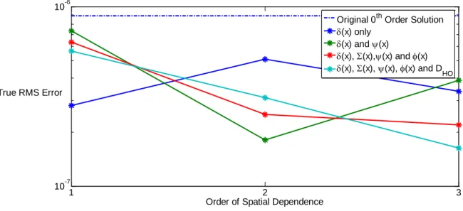
3.7.1 Methods for Using High Order Spatial DGM for Corrections ... 64

3.7.2 Results for 1D Benchmark ... 66

3.8

M

EMORY

C

ONSIDERATIONS FOR

S

PATIAL

R

ECONDENSATION

...68

3.9

S

UMMARY

...70

4

EXACT SPATIAL RECONDENSATION ...73

4.1

D

ERIVATION OF

E

XACT

R

ECONDENSATION FOR

1D

MOC ...73

4.2

1D

B

ENCHMARK

R

ESULTS FOR

E

XACT

R

ECONDENSATION

...76

4.3

C

ONVERGENCE

P

ROPERTIES OF

E

XACT

DGM ...77

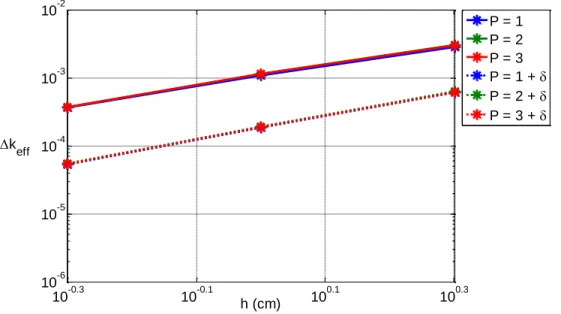
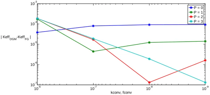
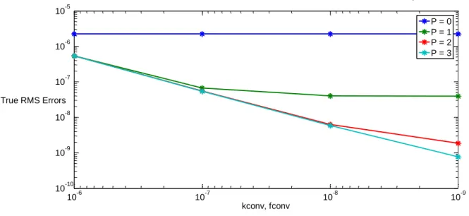
4.3.1 Choosing the Eigenvalue Convergence Criteria ... 78

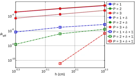
4.3.2 Defining a Natural Del Term ... 90

4.3.3 The Del Term as a Modification to the Streaming Coefficients ... 98

4.4

M

EMORY

R

EQUIREMENTS

...106

4.5

S

UMMARY

...109

9

5.1.1 The Subgroup Decomposition Method ... 115

5.1.2 Fully Consistent Coarse Group Collapse for Recondensation ... 117

5.1.3 Applying the Coarse Group Sweep... 127

5.1.4 Removing the Non-Monotonic Convergence of the Recondensation Process ... 130

5.2

A

PPLICATION TO THE

1D

HTR

AND

1D

MOX

F

INE

G

ROUP

P

ROBLEMS

...135

5.2.1 Effect of Coarse Group Structure ... 137

5.2.2 Coupling to Different Polar Angle Quadratures ... 147

5.2.3 Coupling to Different Spatial/Angular Methods... 152

5.2.4 Application to Linear Anisotropic Scattering in 1D HTR ... 158

5.3

S

UMMARY

...160

6

2D TESTING OF SEAM USING OPENMOC ...163

6.1

A

B

RIEF

I

NTRODUCTION TO

O

PEN

MOC ...163

6.2

N

EW

F

EATURES

I

MPLEMENTED TO

T

EST

SEAM ...165

6.2.1 Group Collapse for Transport Problems ... 166

6.2.2 Gauss-Seidel with Upscatter Option ... 166

6.2.3 Step Difference Transport Kernel ... 167

6.2.4 Fine Group Volumes and Leakage Scaling for the Rayleigh Quotient ... 168

6.3

A

PPLICATION OF

SEAM

TO THE

C5G7

B

ENCHMARK

C

ORE

...169

6.3.1 Energy Acceleration of the C5G7 Benchmark Using SEAM ... 170

6.3.2 Simultaneous Energy-Angle Acceleration ... 175

10

6.4

A

PPLICATION OF

SEAM

TO THE

“C5G361”

C

ORE

...187

6.4.1 Description of the “C5G361” Core ... 187

6.4.2 C5G361 Fine Group Transport Acceleration with SEAM and CMFD ... 189

6.5

S

UMMARY

...193

7

NONLINEAR DGM AND ENERGY PRECONDITIONING ...195

7.1

N

ONLINEAR

D

ERIVATION WITH

E

XPLICIT

R

ECONDENSATION

...197

7.2

R

ESULTS FOR

I

NFINITE

H

OMOGENEOUS

P

ROBLEMS

...204

7.3

N

ONLINEAR

I

MPLICIT

R

ECONDENSATION

...206

7.4

R

ESULTS FOR

I

NFINITE

H

OMOGENEOUS

P

ROBLEMS

...211

7.4.1 Relaxing the Residual Equations ... 212

7.4.2 Discrete Cosine Transforms as a Preconditioner ... 213

7.4.3 Forming a Set of Natural Basis Functions ... 217

7.4.4 Results for Natural Basis Preconditioning ... 223

7.5

R

ESULTS FOR THE

1D

HTR

M

ODEL

U

SING

D

IFFUSION

...227

7.5.1 Preconditioning Using Natural Basis Functions ... 227

7.6

S

UMMARY

...235

8

CONCLUSIONS ...237

8.1

S

PATIAL

R

ECONDENSATION

...238

8.2

E

XACT

R

ECONDENSATION

U

SING

DGM ...239

8.3

T

HE

S

OURCE

E

QUIVALENCE

A

CCELERATION

M

ETHOD

(SEAM) ...240

11

8.5

S

UMMARY AND

F

UTURE

W

ORK

...244

8.5.1 Cheap Improvement of Whole Core Coarse Group Solution ... 245

8.5.2 A Priori Generation of Assembly Level Method Corrected Cross Sections ... 245

8.5.3 Combined SEAM and CMFD Iterations... 246

8.5.4 Unstructured and Heterogeneous Diffusion Acceleration Using SEAM ... 246

8.5.5 Application of Newton Methods to Recondensation Using SEAM ... 246

13

1 Objectives

The end goal of this research is to make a major contribution to the field of high fidelity neutronics analysis through the production of methods and algorithms enabling fine group calculations at the whole core level. In order to achieve this goal, reliance on fine group

transport sweeps to converge the fine group solution must be significantly reduced. The ability to do so in the context of high order spatial methods is also highly desirable to reduce the spatial degrees of freedom. This thesis provides the tools and methods that are key to achieving all of these objectives. However, it is important to understand both what did and did not work. Therefore, details will be provided for all the ideas and thoughts tested, which, while they may not have been breakthroughs in and of themselves, prove useful in formulating an approach that is practical, feasible and nearly universal in its application.

In Chapter 2, the primary issues surrounding whole core analysis with fine group fidelity will be discussed and some of the ways the reactor physics community has approached these issues. Chapter 3 discusses the first steps towards addressing spatial inconsistencies between the Discrete Generalized Multigroup method (DGM) and the original fine group problem and what may be the first successful attempt at producing and incorporating high order spatial cross sections in the context of multigroup collapse. Chapter 4 goes one step further and provides one of the first means of enforcing exact consistency between like spatial methods after energy condensation takes place. Chapter 5 incorporates all the aspects learned from these previous attempts and establishes the Source Equivalence Acceleration Method (SEAM). This new method defines the coarse group cross sections such that exact consistency is maintained throughout recondensation even though the coarse group problem may be using angular quadratures, orders and spatial methods different from those used in the fine group problem. Chapter 6 discusses the implementation of SEAM in OpenMOC and provides initial 2D results for the C5G7 benchmark and a 361 group problem based on the C5G7 core. The results for SEAM in both cases are compared to CMFD, the current state-of-the-art in physics-based

14

acceleration techniques. Chapter 7 then discusses an approach derived from DGM which allows for preconditioning of the energy problem in order to further accelerate convergence.

The ideas proposed in this thesis provide a solid foundation for further acceleration of fine group transport calculations and represent a significant step forward in realizing the goal of fine group whole core analysis.

15

2 Introduction: Multigroup Whole Core Analysis

Achieving high fidelity analysis of reactor neutronics is of utmost importance in analyzing the performance and safety of reactor designs. Since quantities such as power density are directly proportional to fission rate density, which in turn is dependent on the neutron distribution, accurate predictions of the distributions of neutrons in a reactor core are key to performing steady-state and transient safety analyses. These analyses are conducted by solving the neutron transport equation.

The steady-state neutron transport equation is an integral-differential equation which governs the conservation of neutrons moving through any point in space at a certain angle with a particular kinetic energy. In 3D applications, this equation has 6 dependent variables: 3 in space, 2 in angle and 1 in energy. ⃑⃑ ( ⃑⃑ ) ( ) ( ⃑⃑ ) ∫ ∫ ( ⃑⃑⃑⃑ ⃑⃑ ) ( ⃑⃑⃑ ) ⃑⃑⃑⃑ ( ) ∫ ( ) ( ) (2.1)

Ideally, this equation would be solved exactly for a given 3D reactor model including a detailed representation of all reactor internals and their corresponding cross section data. The solution would then provide the number of neutrons at each spatial point in the core moving at a particular angle with a specific kinetic energy. In order to be accurately solved, thermal-hydraulics and fuel performance models must be coupled to the neutron transport solution in order to provide the exact neutronic conditions present in the core.

Many simplifications can be made such that this transport equation becomes solvable. If the neutron is assumed to be mono-energetic, meaning its kinetic energy remains constant, both the spatial and angular dependences can be solved. If the angular distribution is assumed to be only

16

linearly anisotropic, then one can derive a neutron diffusion equation which may be solved using any number of finite difference, finite element, nodal or analytic methods. In this case, the scalar (i.e. angle-integrated) fluxes are provided directly through solution of these equations. On the other hand, if one only wishes to solve this equation over a discrete set of angles, one can derive the discrete ordinates method using various treatments for the spatial dependence, step difference (SD), diamond difference (DD), method of characteristics (MOC), etc. An extra step is required in this case, since one must apply numerical integration across all angles typically using some quadrature to arrive at the scalar flux distribution.

The mono-energetic approximation, however, is extremely poor due to the nature of cross sections governing the various reactions rates. This cross section data is gathered

experimentally, defined by 100,000’s of data points over the energy domain and, for many of the materials used in reactors, the variation of these cross sections are extremely complex. This data may vary by many orders of magnitude, anywhere from 10-5 to 105 barns (10-24 cm2), across an energy domain that can span 12 orders of magnitude, 10-5 eV to 107 eV. The scattering cross section is especially difficult to model accurately due to the coupled nature of scattering between energies and angles.

A stochastic approach can be taken, like in MCNP and OpenMC, in which one essentially creates a neutron and samples across the whole gambit of possible reactions according to the entire set of evaluated nuclear data. [3] Although this can provide extremely accurate analyses for reactor design, the stochastic nature of this solver leads to a standard deviation and thus an uncertainty associated with the solution which decreases only as 1/√ . Here, N represents the number of neutrons interacting with a given cell within the reactor. In order to obtain an accurate representation of the fluxes across the entire core, an extremely large number of neutrons must be simulated. [3][29]

The solution of the neutron transport equation through deterministic methods is computationally cheap by comparison, since a direct solve of the transport equation directly provides the neutron fluxes across the entire reactor. However, an approximation is made which changes the energy dependence from a continuous quantity to a discrete dependence to allow solution of the neutron

17

spectrum in a feasible manner. This is accomplished through application of the multigroup approximation. ( ) ∫ ( ) ( ) ∫ ( ) (2.2)

This approximation is applied through integration of the neutron transport equation across various bounded domains in energy, which are referred to as energy groups. Integration across each of these groups effectively provides the total reaction rates within these energy bounds. These reactions rates are then divided by the integrated fluxes to provide a set of multigroup cross sections. When applied to the continuous energy form of the neutron transport equation, this approximation provides a set of transport equations for each energy group, each of which are directly coupled to one another. These are referred to as the multigroup transport equations.

⃑⃑ ( ⃑⃑ ) ( ) ( ⃑⃑ ) ∑( ) ∑ ∑ ( ) ( ) ( ) ∑ ( ) ( ) (2.3)

One may notice that in the production of these multigroup equations the solution to the

continuous neutron transport equation is assumed to be known a priori. This leads us to a long standing philosophical question closely associated to whether the chicken came first or the egg. In this case, the question then becomes which comes first, the solution or the simplification? Therefore, all methods dealing with energy condensation in some way attempt to address how one obtains an approximate solution which provides an accurate solution using the simplified equations.

18 2.1 Cross Section Generation for Whole Core Analysis

Currently, a multi-level procedure is employed to effectively treat energy dependence in the neutron transport equation. At the first level, an extremely simplified spatial model is used to reduce the number of spatial and angular unknowns solved such that a detailed energy treatment can be undertaken. This simplification can either contain no spatial information, as in the case of an infinite homogeneous calculation, or it can represent the first level of spatial heterogeneity in core, in the case of LWRs this would be a pin cell calculation. In this calculation, the nuclear data can be represented in its original pointwise form or linear-linear interpolation of the pointwise data can also be used to solve for an extremely resolved neutron spectrum. This allows one to account for energy self-shielding effects due to the presence of resonant absorbers and, in the case of the pin cell calculation, spatial self-shielding as well. For example, in an infinite homogeneous calculation, background cross sections from either a moderator or other structural materials can be incorporated into resonance self-shielding models in order to accurately consider the effects of dilution. [15] Pin cell calculations can be used to calculate Dancoff factors in order to approximate the effects of spatial self-shielding due to the presence of fuel in an infinite repeating array. Once these important physics features are captured, energy condensation is used to produce a set of multigroup cross sections. Energy condensation allows the reaction rates from the resolved energy problem to be preserved exactly if the same spectral conditions are present in later calculations. This reduces the number of energy unknowns one needs to solve from 100,000’s to a few hundred, making a more detailed spatial and angular treatment possible for larger, more complex geometries. Though theoretically few group (2-10 groups) cross sections can be produced at this point, this will lead to a very poor approximation in subsequent calculations since the spatial and angular dependence on the energy problem won’t be sufficiently captured

At the second level, an assembly level calculation is conducted solving a few hundred coupled multigroup equations. This analysis incorporates the presence of different fuel enrichments, burnable poisons, control rods, and structural materials within an assembly. This step is incredibly important since any materials with significantly different properties may have a

19

profound effect on the reaction rates in neighboring fuel pins, due to changes in the neutron spectra. Deterministic transport methods are usually applied at this stage to adequately resolve spatial and angular dependencies not present in the ultra-fine group calculation. Once the fluxes are calculated for all the different assembly types present in the full reactor model, energy condensation is applied again, collapsing the few hundred cross sections to 2-8 group cross sections. At this point, homogenization can also be applied either across individual pin cells within the assembly or across the entire assembly to further reduce spatial degrees of freedom. While condensation and homogenization may exactly preserve reactions rates when the

conditions of the assembly calculation match perfectly those in the core, preservation of net currents isn’t guaranteed. This second collapse procedure makes whole core calculations feasibly by countering the increase in spatial scale and complexity through a reduction of the energy degrees of freedom.

At the third level, 2-8 multigroup equations are solved across the whole core geometry using either a low-order angular discrete ordinates approach or solving a diffusion problem. If the assumptions behind all these approximations are satisfied at the whole core level, then the solution will provide an accurate representation of the reaction rates in the core.

This approach still sidesteps the issue of needing the solution beforehand for energy

condensation to preserve reaction rates exactly. If the boundary conditions of the pin cell or assembly do not match those in the full core geometry, then each application of energy condensation will introduce errors into the subsequent calculation. Unfortunately, the best assumption which can be made a priori is that of an infinitely repeating array of the same pin cell or assembly types. If the core is comprised entirely of the same pin cell or assembly type, then this could be a decent approximation. However, this is rarely the case. There will typically be at least 2 or 3 pin cells containing different enrichments and burnups of fuel, but others could possibly contain burnable poisons, fission chambers, water holes, etc. Assemblies of different types may be placed in close proximity to each other as well. In all of these cases, the reflective boundary conditions used to collapse cross sections can’t accurately represent the interactions of ultra-fine group or fine group neutron spectra between differing adjacent materials. [1]

20

Therefore, additional methods have been developed to preserve some accuracy in the multi-level multigroup procedure.

2.2 A Priori Methods

Much of whole core analysis for the current LWR fleet is conducted through application of a priori methods, in which energy condensation is conducted for a single assembly using reflective boundary conditions. This is usually in conjunction with some level of spatial homogenization, either of the full assembly or the individual pin cells within the assembly. While the conditions inside the reactor may not be perfectly represented in these calculations, the approximation is typically assumed to be reasonable if there is no significant change in material properties between neighboring assemblies.

2.2.1 General Equivalence Theory

Generalized equivalence theory provided a practical and very cheap way to reduce errors accrued in the whole core calculation when differing assemblies are placed next to each other. In many of the nodal diffusion calculations conducted at the whole core level, two major constraints were typically applied: continuity of current and continuity of surface fluxes at the boundary between assemblies. However, conservation of neutrons is governed by the assembly averaged scalar fluxes and the net currents at the boundaries. Continuity of the surface scalar flux between assemblies, while providing the additional equations needed to solve the problem, doesn't really factor into neutron balance. Therefore, the surface scalar fluxes are allowed to become

discontinuous between adjacent assemblies. The relaxation of this continuity condition forms the foundation of General Equivalence Theory (GET). [31]

GET's approach to defining these discontinuous surface fluxes is to compare the surface scalar flux from the heterogeneous assembly calculations to the result obtained by using the

homogenized model. The ratio of the heterogeneous to the homogenized surface fluxes provides the discontinuity factor (DF). These DFs are defined using , the surface scalar flux for the heterogeneous assembly calculations, and , the surface scalar flux of the assembly using the cross sections homogenized from the heterogeneous calculation.

21

(2.4)

The general idea behind this approach is that the DF allows surfaces fluxes to be discontinuous in the whole core model so that the surface currents between neighboring assemblies or other homogenized regions can be more accurately captured. For example, in a diffusion calculation, two constraints are placed on the boundaries between two neighboring assemblies, continuity of the surface scalar flux and continuity of the net surface current. Since the surface scalar flux of the homogenized assembly can be much different from that of the heterogeneous assembly, the scalar flux continuity condition in the homogenized problem biases the net surface current values. When DFs are used according to Equation (2.5), the surface scalar flux continuity condition between two adjacent assemblies, A and B, is enforced using their respective DFs, and through multiplication with the homogenous surface fluxes, and . This forms a kind of heterogeneous surface scalar flux continuity condition for the homogenized problem, removing the bias to the net surface currents due to homogenization.

(2.5)

This produced significant improvements in assembly power distributions in whole core

calculations in an extremely cheap manner. These DFs can also be produced by simultaneously homogenizing and condensing the assembly calculation to produce DFs that approximately recreate the conditions of the fine group, heterogeneous assembly calculation. Any number of pin power reconstruction methods could then be used. [31][30]

DFs have been applied to a wide variety of problems in reactor physics calculations due to their flexibility and simplicity. Their application has been extended to produce interface discontinuity factors for individual pin cells to better correct for neighboring effects at the pin cell level, as opposed to assemblies. [17] DFs have also been included in to CITATION for HTR analysis for their ability to better take into account the larger neutron currents at the edge of the reflector and in the vicinity of the control rods. [33]

22 2.2.2 Superhomogenization Method

A slightly different approach can be implemented through a process called

Superhomogenization. For this method, homogenization and condensation occur at the pin cell level within the assembly calculation. Multiplicative factors referred to as Superhomogenization (SPH) factors, , are defined for a cell k by the ratio of the heterogeneous pin cell fluxes, _,

to the pin cell fluxes from the homogenous calculations, _.

(2.6)

Since these SPH factors are determined for each of the homogenized pin cells scalar flux, and not the surface fluxes, these factors can be used to correct the homogenized cross sections for the pin cells.

̃ (2.7)

Although the heterogeneous solution is independent of the SPH corrected cross sections, the changes in the homogenized cross sections cause the homogeneous fluxes to change after each update of the SPH factors. Therefore, an iterative process must be conducted where the cross sections are updated with the SPH factors and new SPH factors are calculated using the updated cross sections. After converging, these factors should provide the necessary corrections to conserve the net current through each cell. It is important to note that there are an infinite number of SPH factors that can conserve reaction rates in this fashion, therefore an additional normalization condition is typically used to provide the closing relation. These factors have been produced at the assembly level to approximately enforce transport (S16) to diffusion equivalence

or transport (S16) to transport (P3) with good success. [4] [14]

In the whole core calculation, fine mesh finite-difference diffusion can be used and these SPH factors applied to their respective homogenized pin cells to enforce what should be better defined pin cell currents. While this does lead to some modest improvements in terms of assembly and pin power calculations, GET still remains the simplest and most widely used a priori approach.

23 2.3 Nonlinear Acceleration Methods

Since a priori methods take a one-size-fits-all approach to approximating whole core solutions in a computationally cheap manner, the spectral interactions between adjacent assemblies may not be accurately characterized, especially if simultaneous homogenization and condensation has occurred. Nonlinear acceleration methods, on the other hand, are able to capture all the spectral swapping but rely on an iterative approach in which full transport sweeps are conducted. While the full transport sweeps are expensive, the problem is solved primarily through the creation and solution of equivalent, yet cheaper, versions of the full problem. These cheaper versions can be formed using spatial homogenization, energy condensation and/or a low order angular

approximation. The solutions from these equivalent problems are then used to reduce the total number of full transport calculation required to converge the fission source. This provides a relative cheap process by which the true solution of the whole core problem can be obtained. While this requires extra work relative to an assembly level calculation conducted before the fact, this provides the true solution through application of fewer full transport calculations. 2.3.1 Diffusion Synthetic Acceleration

In the early days of deterministic transport solvers, diffusion synthetic acceleration (DSA) was the primary method of use in accelerating convergence of transport problems. In DSA, an inconsistent diffusion problem is used to provide an estimate of the error between successive transport iterations (within-group or power iteration). This estimated linear error is then used to correct the transport solution to provide an acceleration of the scalar flux for the next iteration. Equation (2.8) provides an example of its use in accelerating within-group convergence. The intermediate current and fluxes are calculated using the solution from the previous transport sweep.

⁄ ⁄ (2.8)

For Equation (2.8), Dg denotes the diffusion coefficient for coarse group g, ΣR,g is the total

24

The parameters ⁄ and ⁄ are the current for group g and scalar flux for group g respectively as calculated from the intermediate transport solution. The diffusion problem in Equation (2.8) is solved to provide the fully updated scalar flux, _{, for the next transport}

calculation.

This diffusion flux would accelerate the transport solution by providing a cheap means of improving the scalar flux spatial distribution. However, energy condensation and spatial homogenization were never really folded into DSA.

2.3.2 Simultaneous Homogenization and Condensation

Coarse mesh rebalance (CMR) is another method by which a simpler problem is solved but forced to be consistent with the high order angular problem. This approach, though, is typically focused on accelerating the spatial and angular complexity of high order problem, not necessarily the energy aspect. CMR not only simplifies the angular aspect of the problem, but it also

incorporates spatial homogenization. A flux and volume weighted average is applied to cross sections across a collection of cells to form a larger, homogenized cell, thereby reducing the number of spatial degrees of freedom. Neutron conservation is maintained in this process by using the basic neutron balance equation and multiplying the incoming currents at the coarse mesh boundaries by a set of rebalance factors. Application to a 1D problem is highlighted in Equation (2.9). Index i denotes the coarse mesh, index k denotes a cell within coarse mesh i and l denotes the current iterate of the solution. The currents at the boundaries of cell i, ⁄ and

⁄ _{, along with the cell averaged scalar flux,} ⁄ _{, and the cell averaged source,}

, are forced into exact neutron balance by solving for rebalances factors for each cell, _.

( ⁄ ⁄ ∑ ⁄ ) ⁄ ⁄ _∑ (2.9)

25

Once these rebalance factors are calculated for the previous high order iterate, the angular fluxes at the coarse mesh boundaries and the cell-averaged scalar fluxes are accelerated

accordingly. This significantly reduces the total number of transport sweeps required to achieve the given tolerance. Since this approach uses a general neutron balance equation, it can be easily applied to structured and unstructured geometries.

Unfortunately, CMR is not without issues. This nonlinear approach is only conditionally stable. In many cases, when the coarse mesh is optically thick or thin, the acceleration scheme diverges. [7] However recent developments such as Coarse Mesh Angular Dependent Rebalance (CMADR) have been implemented and shown to be unconditionally stable. This approach adds additional degrees of freedom to the coarse mesh problem being solved [26][27]

Coarse mesh finite-difference (CMFD) diffusion is another widely used nonlinear acceleration scheme. In this case, the high order angular problem is represented by a low-order diffusion problem. Equivalence is enforced through the addition of current correction factors. These take on the shape of an additional set of diffusion coefficients which modify the original

coefficients. These current correction factors are calculated using the net surface currents for cell i, _⁄⁄ , the coarse mesh scalar fluxes, ⁄ and ⁄ , and the normal diffusion coefficient coupling the two coarse meshes, ̃ ⁄ . This current corrective factor between the

meshes, ̂ ⁄ , produces a diffusion problem equivalent to the transport problem. Not only can

Equation (2.10) take into account spatial homogenization, but it can also include energy condensation, to create a cheaper version of a fine group transport calculation.

̂ _⁄ ⁄⁄ ̃ ⁄ ( ⁄ ⁄ ) ⁄ ⁄

(2.10)

Once the current correction factors are calculated, a set of finite-difference diffusion equations are solved to provide the updated fluxes for each of the coarse meshes.

26 ( ̃ ⁄ ̂ ⁄ ) ( ̃ ⁄ ̂ ⁄ ) ( ̃ ⁄ ̂ ⁄ ̃ ⁄ ̂ ⁄ ) ∑ (2.11)

The updated coarse mesh fluxes are then used to scale the previous iterate of the fine mesh fluxes, thereby accelerating the transport problem. While this tends to accelerate transport solutions faster than CMR, it is slightly limited in application since the typical finite difference approach is more intuitive when applied to problems using structured meshes. However, recent generalizations of CMFD to unstructured meshes have been derived and used to accelerate transport calculations as well. [19] CMFD’s applicability has even been extended to monte carlo codes by accelerating the convergence of the fission source distribution. [22] This acceleration of the fission source has also been included into OpenMC with the added functionality of

estimating dominance ratios. [16]

CMFD also suffers from the conditional stability issues observed in CMR. In the case of CMFD, however, this usually only occurs for coarse meshes which are optically thick. The best

performance in CMFD is typically observed when applied to optically thin coarse meshes. If CMFD is able to converge for an optically thick problem, little to no acceleration is observed. [21] In many applications of CMFD, a damping factor is applied to prevent such instabilities from growing and causing divergence. This damping factor is largely problem dependent but a reasonable value can be applied across a number of different problems. Partial current Coarse Mesh Finite Difference (pCMFD) is a more recent development which has also been shown to be unconditionally stable and used to accelerate MOC calculations in the NEWT transport code. This approach adds a second degree of freedom to CMFD, allowing it to create two partial current corrective factors at the boundaries of a coarse mesh instead of just recreating a single net current corrective factor. [19][18]

Generalized coarse mesh rebalance has been recently shown to bridge the gap, so to speak, between CMR and CMFD. In the derivation of GCMR, it was shown that both CMR and CMFD

27

are specific cases of the generalized method. This method employs a generic parameter which can be varied across a wide range of values to produce better stability than could be otherwise achieved in CMR or CMFD alone. The choice of this parameter still requires some fine tuning and the optimal choice is likely problem dependent. However, the CMFD-like method produced with GCMR tends to be very close to optimal choice for this parameter in many cases and, through this methodology, can be applied to unstructured meshes. [35]

2.3.3 Recent Developments

More recent approaches focus solely on maintaining exact consistency between a fine group and coarse group calculation. One example is a PHYSOR 2002 paper looking at enforcing

consistency in the context of MOC. In order to enforce exact consistency, the outgoing coarse group angular fluxes were forced to match the collapsed fine group outgoing angular fluxes through application of discontinuity factors for each angle, segment and coarse group. This led to significant deficiencies in performance since the memory overhead became huge for larger problems. However, this method did show that it was possible to achieve full consistency, albeit at the cost of memory. [5]

A more promising approach was developed by Lulu Li at MIT. This approach formulates a low order MOC transport calculation using quadrant space-angle domains with equal weights across a pin cell homogenized problem. A low order problem equivalent to the main MOC calculation is then set up by tallying the quadrant currents at each of the pin cell surfaces. An equivalent low order source is then calculated for each of the 8 coarse mesh tracks inside each pin cell to

preserve the incoming and outgoing quadrant angular fluxes. Once this lower order problem is constructed, it can then be solved and used to accelerate the high order MOC calculation. This demonstrated very good acceleration of the C5G7 benchmark, even significantly improving upon the normal CMFD approach already incorporated into OpenMOC [23]

Another approach to achieving consistency was conducted through the use of angular dependent total cross sections. These were calculated by collapsing the fine group total cross sections using the cell-averaged angular fluxes instead of the scalar fluxes. This was successfully applied using

28

diamond difference discrete ordinates and shown to converge to the fine group solution in that case. A reduction of the angular order by collapsing the angular problem was attempted to minimize storage costs associated with an angular dependent cross section. The result was a reduction of the high order angular quadrature to a sort of S2 calculation using a spatially varying

average cosine angle. While this approach is certainly interesting, inconsistencies lead the method to converge to the incorrect solution when the angular dependence of the coarse group total cross section was treated as an anisotropic source. [6]

2.4 Recondensation

Recondensation is slightly different from the typical nonlinear acceleration method. Rather than homogenizing and condensing a fine group problem, the focus is placed on accelerating the energy problem while staying on the same spatial discretization. Ideally, acceleration would be achieved by solving an equivalent coarse group eigenvalue problem and then using an additional method to provide a way to reconstruct the previous fine group solution using the coarse group solution. The reconstructed fine group flux would be an improved solution and subsequently used to produce new coarse group constants for another coarse group solve. If the coarse group problem and reconstruction process are equivalent to the fine group problem, then iteration of this process will lead to the fine group solution. Currently, there are two primary methods which allow for direct reconstruction of fine group fluxes: the Subgroup Decomposition Method (SGD) and the Discrete Generalized Multigroup Method (DGM).

2.4.1 Subgroup Decomposition Method (SGD)

The SGD method proposed by researchers at Georgia Tech will be covered more in-depth in Section 5.1.1.

2.4.2 Discrete Generalized Multigroup Method (DGM)

DGM is essentially a discrete form of the Generalized Energy Condensation (GEC) method, which applied a transformation through a series of continuous polynomial functions to the

29

produce a set of moment equations, referred to as DGM equations, to better represent the discrete nature of the multigroup cross sections. Once solved, these equations produce a set of flux moments which can then be used to reconstruct fine group fluxes. Sections 2.4.2.1 through 2.4.4.2, will cover the derivation, properties and usage of DGM in the context of recondensation in detail.

2.4.2.1 Derivation and Properties of DGM

Using the multigroup approximation in the group collapse process, it is assumed that the fine group spectrum within each coarse group is flat. In doing so, all information about the fine group spectrum is lost. With DGM, it is assumed that the spectrum within each coarse group is expanded using a set of orthogonal functions. While continuous functions in energy can be used to represent the fine group spectrum [28], discrete basis functions are a more natural fit for the discrete nature of the multigroup equations and constants. This discrete representation of the within-group fluxes provides the basis for the formation of the DGM moment equations. The fine group flux can be expanded in terms of these discrete basis functions within the traditional multigroup equations. After this expansion, the resulting equation is dependent on all the moments. To decouple these flux moments, the equation is multiplied by the ith discrete basis function and summed. This process produces the DGM moment equations shown in Equation (2.12). [40] Although this process also works for anisotropic sources, for the purpose of this thesis, it is assumed that only isotropic scattering is taken into account.

⃑ ( ⃑ ) ( ⃑ ) ( ⃑ ) ( ⃑ ) ( ⃑ ) ∑ ( ) ( ) ( ) ∑ ( ) ( ) (2.12)

30

One may notice that the multigroup constants have been redefined in Equation (2.12). This is required so that the source calculated is transformed into the same basis as the fine group flux. In this transformation, reaction rates must also be conserved. This transformation can’t simply modify the fine group cross sections themselves, but must also take care to conserve the reaction rates from the fine group problem. Therefore, the fine group reactions rates are multiplied by the discrete basis functions before carrying out the typical multigroup collapse.

( ) ∑ ( ) ( ) ( ) ∑ ( ) ( ) ⁄ _(2.13) ( ) ∑ ( ) ( ) (2.14)

One thing to notice is that, while the definition of the fission cross section remains unchanged, the fission spectrum has been transformed using the discrete basis functions. This is because the shape of the chi spectrum is not influenced by the incoming spectrum. Only the magnitude of the outgoing fine group spectrum changes according to the total fission rate. Therefore, the summation over incoming energy groups, L, can be separated from the summation over the outgoing energy groups, K, leading to the numerator of Equation (2.13) and Equation (2.14). The coarse group fission rate on group g’ is then normalized by the total flux in group g’ to preserve the fission reaction rate. Since chi is not technically reaction rate but a spectrum, no weighting of the chi spectrum by the scalar flux is necessary in the case of energy condensation. Only the spectrum itself needs to be transformed by the discrete basis function such that the basis

representing the source matches that of the flux moments.

( ) ∑ ∑ ( ) ( ) ( ) ∑ ( ) ⁄ _(2.15)

The scattering cross section looks a bit different, though. Instead of the neutrons scattering from an initial fine group L to outgoing fine group K, they scatter from an initial coarse group g’ to coarse group g and moment i. This is because the incoming energy of the scattering cross section is collapsed using the fine group flux to preserve reactions rates. Once the incoming

31

energy has been collapsed to their respective coarse groups, this still leaves the outgoing fine group K. This is weighted by the discrete basis functions before collapsing the outgoing energy. Coarse group fluxes can then be used to produce a fine group source, but one which has been transformed into the same basis as the flux moments.

( ⃑ ) ∑ ( ) ( ⃑ ) ( )

∑ ( ) ( ⃑ )

⁄ _(2.16)

On top of the total source on the RHS of the transport equation, conservation of the streaming and removal operators must also be ensured. The streaming term itself does not explicitly depend on the energy and so the summation over the discrete basis function only produces the flux moments inside the streaming operator. However, the total removal reaction rate still needs to be conserved. The fine group total cross sections are weighted by the angular flux and

collapsed to produce the cross sections. Alternatively, the scalar flux could be used to provide a coarse group total cross section, but for now the angular dependent definition will be used.

( ⃑ ) ∑ ( ) ( ⃑ ) ( )

∑ ( ) ( ⃑ )

⁄ _(2.17)

One may notice that the total cross section was not defined using the discrete basis functions. There are two main reasons for this. First, if the moment total cross sections were defined using the flux moments as defined in Equation (2.17), the summation on the denominator could potentially become zero since only the 0th order moment flux is guaranteed to be positive. This could occur if the fine group spectrum is flat within a coarse group. The first order moment total cross section would then be divided by the linear component of the spectrum, which would be zero in this case. Since computers, like human beings, tend to not like dividing by zero or numbers close to zero, this should absolutely be avoided. If left unaccounted for, this issue can lead to accrual of round off errors or divergence of the solution. Second, the use of discrete basis functions to represent the moment total reaction rates, the numerator of Equation (2.17), can result in a negative moment total cross section. This might occur if the linear component of the total reaction rates has a slope opposite that of the flux. If this is the case and a method such as

32

Step characteristics or MOC were being used, then the resulting solution of the first order differential transport equation produces exponential growth in the moment angular flux instead of exponential decay, possibly leading to further instability. [40] To prevent these issues the coarse group total cross sections are used for all the moment equations within a coarse group since these cross sections are always positive and finite. However, a new term must be

introduced to account for the difference between using the coarse group total cross section and the moment total cross section.

( ⃑ ) ∑ ( ) ( ⃑ ) ( ( ) ( ⃑ ))

∑ ( ⃑ )

⁄ _(2.18)

Since the coarse group total cross section is used, one can’t define a distinct total cross section for each moment. A corrective term must be used that can account for this inconsistency. This is where a new term, the del term, comes into play. The del term incorporates a correction to the LHS of the DGM equations by collapsing the difference between the fine group and coarse group total cross sections. This can then be moved to the RHS of the transport equation and be treated like an angularly dependent source term.

At this point, there are still as many equations as the original fine group problem, but what has changed is how these equations are used. With DGM, the power iteration only needs to be conducted on the 0th order DGM equation. This is because all of the integrated reaction rate information is contained within the 0th order equation. Another nice feature is that the del term vanishes for the leading moment equation and reduces to the traditional coarse group equation. Therefore, instead of having to conduct the power iteration over all the fine group equations, this only has to be done for the coarse group equations.

( ) (2.19)

This by itself does not lead to an improved solution, since this still only produces a coarse group solution with the same limitations as before. However, the higher order DGM equations only depend on the coarse group scalar and angular fluxes. Therefore, once the coarse group solution has converged, these fluxes can be used to produce the sources for the higher order DGM

33

equations. All that’s left to do is solve a set of fixed source problems to calculate the rest of the angular flux moments.

( ) (2.20)

If the moment cross sections have been properly defined for the problem, then the angular flux moments can be used to reconstruct the exact fine group solution.

( ⃑ ) ∑ ( ) ( ⃑ )

(2.21)

2.4.3 Discrete Basis Functions

Before continuing further, it is important to discuss the choice of discrete basis function that is used to transform the original fine group equations into the DGM equations. The accuracy to which these basis functions can be constructed will in turn limit the ability of DGM to

reconstruct fine group fluxes in a trustworthy manner. 2.4.3.1 Discrete Legendre Polynomials

Previous work focused primarily on using the Discrete Legendre Polynomials (DLP’s) as the basis for the DGM equations. This basis is essentially the discrete analogue of the continuous Legendre Polynomials. [21] To build these DLPs, a second order recurrence relation defined by Equation (2.22) is used.

( )( ) ( )

( )( ) ( ) ( ) ( )

(2.22)

This relation is seeded with the initial values ( ) and ( ) ( ) ⁄ where N is the total number of discrete basis functions and both K and m vary from 0 to N-1.

34

For use in DGM, normalization constants must be computed for the reconstruction of our fine group fluxes. For DLPs, these constants are defined according to Equation (2.23).

( ) ( )

( )( ) ( ) _{( )( ) ( )}

(2.23)

Unfortunately, forming the DLPs using this recursive relation accrues a significant amount of roundoff error for N >50. This is observed in Figure 1 which shows the inability of the DLPs to reconstruct a vector of random numbers using Equation (2.22). The resulting loss in

orthogonality between the higher order basis functions leads to erroneous solutions when solving the DGM equations or even failure to converge.

2.4.3.2 Discrete Tchebyshev Polynomials

The use of Discrete Tchebyshev Polynomials was also proposed previously for use in DGM. These basis functions were shown to have much more favorable properties relative to the DLPs with regard to the accrual of roundoff error. This set of discrete basis functions is also defined using a recurrence relation. [42]

( ) ( ) ( )( ) ( ) ( ) ( ) (2.24) However, the generation of discrete basis function through use of recurrence relations was dropped altogether in favor of a more direct calculation of the elements describing such a function. This was achieved through use of the Discrete Cosine Transform (DCT). 2.4.3.3 Discrete Cosine Transform

In this work, a different set of discrete basis function is used, the Discrete Cosine Transforms of Type II (DCT), for use in the DGM equations. Normally applied to problems such as JPEG file compression, the quality that makes this type of DCT suitable is that the 0th order basis is a vector of 1’s, which makes the leading order DGM equation still identical to the coarse group problem. [1] This type of DCT is defined by Equation (2.25).

35

( ) ( ( )) (2.25)

The normalization constants for these DCTs are much more straightforward to calculate as well.

{

Since DCTs can be built from directly evaluating cosine functions, any round off errors potentially accrued by using a recursive relation are eliminated. The only errors introduced while forming the DCTs are therefore limited to the approximations used in evaluating the cosine functions.

2.4.3.4 Best Choice of Discrete Basis

Ideally, the choice of discrete basis function should be able to expand an arbitrarily large number of fine groups within a coarse group without introducing errors into the reconstruction process. Since the orthogonality of the discrete basis functions is required to ensure accurate

reconstruction of the fine group flux, then the best choice should maintain orthogonality

regardless of the number of fine groups reconstructed. Therefore the ability of both DCTs and DLPs to reconstruct fine group fluxes were tested in the following manner.

1. Multiply a vector, B, by a matrix, P, whose columnspace is comprised of the basis functions

2. Multiply the resultant vector by the transpose of P

3. Multiply by a diagonal matrix, a, comprised of the normalization constants for each function

4. Subtract the final product from the original vector ( ( ))

36

Here, P, can be any discrete basis function, but from now on the discrete basis functions will be referred by their names, DLP and DCT, which are already normalized.

If the number of basis functions, N, matches the length of our vector, B, and the discrete basis functions are exactly orthogonal to one another, the errors accrued should be on the order of machine precision. The following figure shows the results of this test using a vector of 100 random values varying from 0 to 1.

Figure 1 : Comparison of errors accrued using Discrete Legendre Polynomials and Discrete Cosine Transforms

While DLPs cannot reconstruct B to any reliable accuracy, as shown in Figure 1, DCTs can reconstruct all values of B to near machine precision. This is an unfair comparison, though, since the issue with orthogonality in our DLPs was already known beforehand. To be fair, the Modified Gram-Schmidt process was applied to re-orthogonalize the DLPs once the recursion relation has been used. While this improved the reconstruction of B, the combination of Modified Gram-Schmidt with DLPs still did not match the performance of the DCTs. It is important to recognize, however, that for reconstruction of a few fine groups within a coarse group, DLPs and DCTs perform similarly. Though, since the goal is to extend this application to

37

larger numbers of fine groups (on the order of 100s) for any given coarse group, DCTs is no doubt the best option.

Another very nice quality of DCTs is their ability to act on a vector in O(n log(n)) operations using Fast Fourier Transform methods instead of the usual O(n2) number of operations. While for few fine groups this won’t enhance the performance, it could prove extremely useful in preparing cross section data when using DGM to reconstruct 100’s of fine groups within a single coarse group. Therefore, for the rest of our study, DCTs will function as our primary discrete basis function for use in DGM.

2.4.4 Recondensation with DGM

An important observation to note is that DGM by itself can’t fully account for all spectral swapping at the whole core level. No matter how accurately the discrete basis functions can be evaluated, a single solve of the DGM equations still can’t produce the exact fine group solution without knowing the true solution a priori. The root of this limitation is in the fine group spectrum used beforehand to collapse all of the moment cross sections. Even when using the moment cross sections and del terms provided by an assembly calculation, solving the DGM equations will still lead to an incorrect, albeit better, reconstructed fine group flux. Since the spectral boundary conditions for each assembly in the core aren’t known a priori, the reaction rates and therefore the cross sections for all the DGM equations are not representative of the true problem. Unfortunately, the correct calculation of our cross section moments assumes a priori knowledge of the true fine group solution. Since nothing is gained from applying the DGM equations if the fine group eigenvalue problem has already been solved, another method is required. This led to the development of a process called recondensation.

2.4.4.1 Implementation Using DGM

To initialize the recondensation process, an initial guess is assumed for the fine group fluxes and used to calculate the cross section moments. This guess could be the result of an assembly level calculation, an infinite homogeneous calculation or simply a flat flux approximation. With these

38

cross sections, the power iteration is applied to the coarse group equations and the coarse group flux is used to solve the higher order DGM equations. With the new flux moments a new set of fine group fluxes is reconstructed. One additional step is added in which these reconstructed fine group fluxes are used in energy condensation to obtain a new set of moment cross sections.

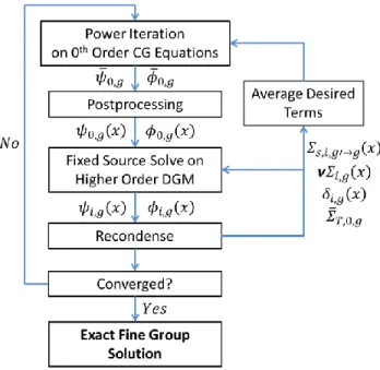
Figure 2 : Flowchart for the recondensation procedure

These updated cross sections are used in the next DGM calculation, the fine group fluxes reconstructed and the process is repeated. After a number of recondensation steps, the reconstructed fine group fluxes will converge towards the true fine group solution. This nonlinear iterative process, highlighted in Figure 2, is called recondensation. [41] 2.4.4.2 Stability and Use of Krasnoselskii Iteration

Initially, recondensation suffered from stability issues which led to divergence in many cases. This instability was first resolved by incorporating a second sweep into recondensation. One would take the fine group fluxes reconstructed form the DGM equations, construct a new fine group source with them and then carryout another transport sweep using the original fine group equations. [41]

39

Ideally, the recondensation process would be performed without need for any fine group sweep, which was resolved by using a Krasnoselskii iteration on the updated angular flux moments instead of employing the typical Picard Iteration. Gibson and Forget (2012) recast the recondensation process into operator notation and the Krasnoselskii iteration was applied to stabilize recondensation according to Equation (2.26).

( ) (2.26)

Here, T denotes the original recondensation process in operator form, k is the current iteration and lambda may vary from 0 to 1. The choice of lambda, of course, is problem specific, and a correct value will provide stability to the recondensation process, allowing it to converge to the true fine group solution. [12]

41

3 Approximate Spatial Recondensation

Much of the work conducted using DGM has been applied to low order spatial methods, such as step difference Sn. The recondensation process has already been shown to converge to the fine

group solution with errors on the order of the convergence criteria set for the problem. [41] Unfortunately, when moving towards application to higher order spatial methods, DGM no longer converges to the exact fine group solution. In this section, this problem is approached through explicit inclusion of the spatial dependence from the angular and scalar fluxes. To do this, however, requires use of high order spatial methods. Therefore, a 1D High Order Method of Characteristics (HOMOC) method is developed that achieves arbitrarily high order. This will then be used to include spatial dependences from the fluxes directly into the cross sections when group collapse is conducted. These high order spatial cross sections will then be used in a high order spatial version of the DGM equations, which should then account for much of the spatial information that is typically lost in the recondensation process when using higher order methods.

3.1 Spatial Inconsistencies in DGM

Spatial inconsistency in DGM is a direct result of the assumptions placed on the shape of the angular flux. In step difference, no shape is assumed in the calculation of the cell averaged fluxes. Therefore, the “shape” set by the streaming and removal operator is equivalent for both the fine group and DGM equations.

In the Method of Characteristics (MOC), for example, the spatial variation of the angular flux in a given cell is defined by an exponential shape. In the original fine group equations, these

exponential shapes are dictated by the value of the fine group total cross section. Therefore, each of the fine group angular fluxes has a different exponential shape.

42

The sweeping operator in the DGM equations, however, is identical across all moments since it uses the coarse group total cross section. This means that the same exponential shape is used to calculate the angular flux moments for each coarse group.

( ⃑ ) ⃑ ( ⃑ ) ( ⃑ ) ( ⃑ ) ( ⃑ ) ( ⃑ ) (3.2)

While the del term that is added to try to correct for the difference in the sweeping operator, the del term is typically moved to the right hand side of the transport equation and treated as a flat source correction. This is what leads to the discrepancy between the original fine group

equations and our DGM equations. The incorrect shapes assumed in DGM can’t be corrected by the current definition of the del term. The lack of spatial information inside the del term

introduces errors into the recondensation process, leading the method to converge to an incorrect solution.

Figure 3 : Comparison of angular flux solution using the original fine group equations and the DGM equations

Figure 3 provides an example of this issue when using a characteristic type method. For the fine group case, the shapes of the angular fluxes are dependent on the total fine group cross sections. DGM, on the other hand, can only use the coarse group total cross section to define the

43

exponential shapes used in the calculation and therefore the same shape is applied across all moments within the same coarse group.

The consequences of this inconsistency can be seen in Figure 4. This plot provides a direct comparison of the recondensation process applied to both step difference Sn and MOC

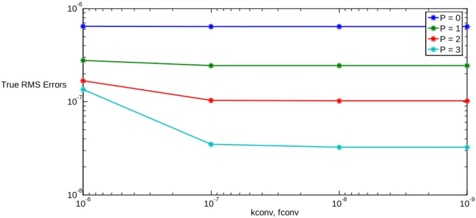
(equivalent to step characteristics in 1D) for the 47 group 1D BWR example problem defined in Appendix B. Using each of these methods, the errors in the recondensation solution relative to the fine group reference case are compared. The convergence profiles are also compared when using various convergence criteria for the fine group problem and the recondensation problem. This provides a good picture of whether or not DGM is consistent with the current spatial method being applied. If the spatial method being used in recondensation is consistent, then tightening the convergence criteria will result in a smaller difference between the reference case and the converged solution. If the method is inconsistent, then the deviation of the converged solution will reach an asymptotic value even though the convergence criteria are tightened further.

Figure 4 : Recondensation with varying convergence criteria using step difference and step characteristics

For the step difference method, as the convergence criterion for keff and fluxes is decreased, the

difference between the fine group and DGM solution decreases. This shows that DGM can be applied to step difference Sn in a fully consistent manner. As predicted before for step

characteristics, the errors in the recondensation solution approach an asymptotic value even when the convergence criteria are tightened.