Aerodynamic performance measurements in a counter-rotating aspirated compressor

(1)

Aerodynamic Performance Measurements in a Counter-Rotating Aspirated Compressor

by

Jean-Franeois Onnee

Ingenieur des Arts et Manufactures (2003) Ecole Centrale Paris (Chatenay-Malabry, France) Submitted to the Department of Aeronautics and Astronautics

in Partial Fulfillment of the Requirements for the Degree of Master of Science in Aeronautics and Astronautics

at the

Massachusetts Institute of Technology June 2005

A uthor... ... ... . .. ... Department of Aeronautic nd Astronautics

May 20, 2005

Certified by...

Accepted by...

Professor Alan H. Epstein R.C. Maclaurin Professor Department of Aeronautics and Astronautics Thesis Supervisor I... MASSACHUSETrSLIN)SYTIE OF TECHNOLOGY

JUN 2

3 2005

LIBRARIES

(2)

(3)

Aerodynamic Performance Measurements in a Counter-Rotating Aspirated Compressor

by

Jean-Franeois Onn~e

Submitted to the Department of Aeronautics and Astronautics on May 20, 2005, in partial fulfillment of the

requirements for the Degree of

Master of Science in Aeronautics and Astronautics

Abstract

This thesis is an experimental investigation of the aerodynamic performances of a counter-rotating aspirated compressor. This compressor is implemented in a blow-down facility, which gives rigorous simulation of the characteristic aerodynamic parameters in which a compressor operates in steady state conditions. To measure the efficiency of this unique machine, the total temperature as well as the total and the static pressures at the inlet and the outlet of the compressor are measured.

Due to the short test time (~100 ms) and unsteady nature of the blow-down environment, performance measurements in a short-duration test facility place especially demanding requirements on the accuracy and the response of the temperature and pressure sensors. For the total temperature probes, 0.0005-inch-diameter type-K thermocouple gage wires were assembled in specially designed casings allowing to perform measurements at determined span and circumferential locations. As for pressure probes, ultraminiature piezo-resistive transducers were used. The uncertainties related to their performances is estimated.

These results are then processed to obtain an estimation of the uncertainties in the efficiency measurement. The error related to the time-resolution as well as the discrete spatial sampling pattern are also assessed. The blow-down test facility provides a quasi-isothermal environment. The non-adiabatic effects lead to a biased efficiency measurement. A corresponding correction to estimate the adiabatic efficiency of the compressor is detailed. Finally, results from the first compressor test runs are provided.

Thesis Supervisor: Alan H. Epstein

Title: R.C. Maclaurin Professor of Aeronautics and Astronautics Director of the Gas Turbine Laboratory

(4)

(5)

Acknowledgments

I would like to thank Professor Alan H. Epstein and Dr. Gerald R. Guenette for

having given me the opportunity to work on this innovative project. I am very grateful for their guidance, support and kindness during the course of this experimental work.

I would like to thank all the members of the blow-down counter-rotating aspirated

compressor team, namely Professor Jack L. Kerrebrock, Dr. Ali Merchant, Dr. Fritz Neumayer and my fellow research student David V. Parker, for their teachings, support and precious help.

Many thanks to Jack Costa, Viktor Dubrowski and James Letendre for their help, patience and skills in turning my drawings into actual probes. I am also grateful to the entire GTL staff for their kindness.

I cannot express enough gratitude to my parents and my sister, whose love and

support gave me the opportunity to earn this degree. I would like to address a special thought to my regretted grand-mother Mamama, for her love and supporting prayers throughout my studies.

Finally, I would like to thank all my friends, overseas, for their support, and here in the United States, for making these two years in New England a great experience.

This work was supported by the Defense Advanced Research Projects Agency, Dr. S. Walker, Manager.

(6)

(7)

List of Figures

Figure 1.1 -Effect of suction on boundary layer growth...20

Figure 2.1 - Inlet Guide Vane Mounted on Forward Section...25

Figure 2.2 - Rotor 1... 26

Figure 2.3 - R otor 2... 27

Figure 2.4 -Bleed Flow Passage in a Rotor 2 Blade... 27

Figure 2.5 - The MIT Blow-Down Compressor Facility... 29

Figure 2.6 - Forward Test Section... 30

Figure 2.7 - Aft Test Section... 31

Figure 2.8 - Instrumentation Positions on Test Stand... 34

Figure 3.1 - Thermocouple Circuit with External Reference Junction...41

Figure 3.2 - Ice Point Reference Chambers...41

Figure 3.3 - Thermocouple Head Design... 43

Figure 3.4 - Infinite Cylinder with Initial Uniform Temperature Subjected to Sudden Convection Conditions...44

Figure 3.5 - Compressional Heating in the Blow-Down Seen by the Upstream Probes.. 47

Figure 3.6 - Downstream Temperature Probe Mounted on Brass Plug... 48

Figure 3.7 - Fully assembled upstream total temperature rake...50

Figure 3.8 - Schematic of Free Jet Resistance Test...51

Figure 3.9 - Picture of 0.0005-inch Thermocouple Gage...52

Figure 3.10 - Gage Wire Shapes Tested in the Free Jet Stand... 52

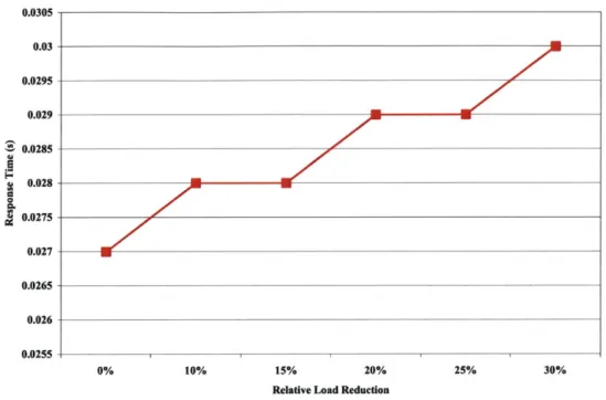
Figure 3.11 - Wire response-time in (s) versus the Percentage of Load Reduction for " heads by Decreasing the Vent Hole Size... 54

Figure 3.12 - Evolution of the Recovery Error versus the Percentage of Load Reduction for " heads, by Decreasing the Vent Hole Size... 54

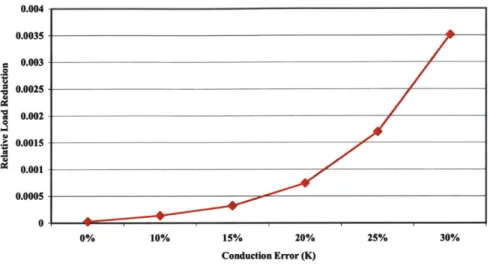
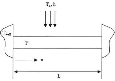
Figure 3.13 - Evolution in Conduction Error versus the Percentage of Load reduction by Decreasing the Inlet Area of a " head... 55 Figure 3.14 - Schematic of One-Dimensional Conduction-Convection Model for

(12)

Figure 3.15 - Conduction Error Percentage, Predicted by a Steady State

One-Dimensional Conduction-Convection Model... 64

Figure 4.1 - Fully-Assembled Upstream Total Pressure Rake...70

Figure 5.1 - Inlet and Outlet Relative Entropy Variations... 83

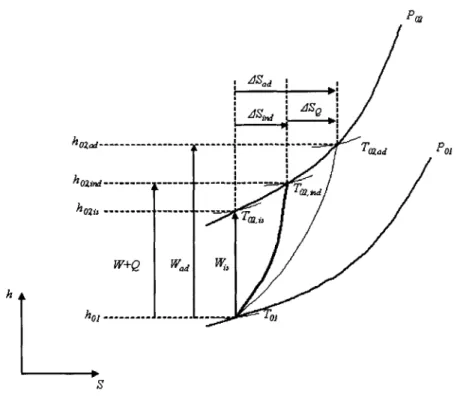
Figure 5.2 - Enthalpy - Entropy Diagram for the Compression Processes in C om pressors...85

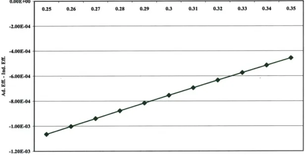
Figure 5. 3 - Difference Between Adiabatic and Indicated Efficiency Over the Test T im e... . . 89

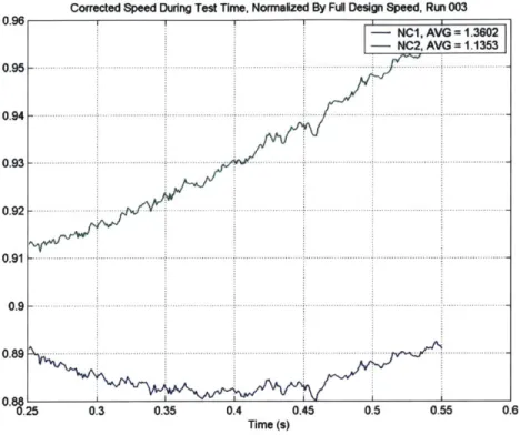
Figure 6.1 - Corrected Speeds During Test Time Normalized by Full Design Speed -R un 003 ... 93

Figure 6.2 - Upstream Total Temperatures of Run 010... 96

Figure 6.3 - Downstream Total Temperatures of Run 010... 96

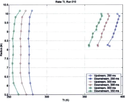
Figure 6.4 - Upstream and Downstream Radial Total Temperature Distribution at 250 ms, 300 ms and 350 ms for Run 010...97

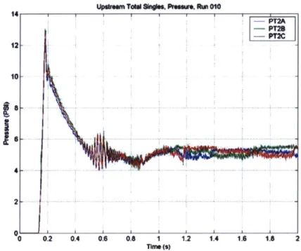
Figure 6.5 - Area-Averaged Pressure History in the Supply Tank, the Valve, Upstream and Downstream of the Compressor, in the Bleed Flow and in the Dump Tank for Run 010... 97

Figure 6.6 - Upstream Total Pressure at Three Midspan Locations for Run 010... 98

Figure 6.7 - Upstream Static Pressure Distribution for Run 010... 98

Figure 6.8 - Upstream Pitot Total and Static Pressures for Run 010... 99

Figure 6.9 - Downstream Pitot Total and Static Pressures for Run 010...99

Figure 6.10 - Upstream Total Pressure Rake Measurements for Run 010... 100

Figure 6.11 - Downstream Total Pressure Rake Measurements for Run 010... 100

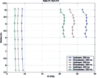
Figure 6.12 - Upstream and Downstream Radial Total Pressure Distribution at 250 ms, 300 ms and 350 ms for Run 010... 101

Figure 6.13 - Pressure Ratio, Temperature Ratio and Efficiency Radial Distributions at 250 ms, 300 ms and 350 ms for Run 010... 101

(13)

Figure 6.14 - High Speed Static Pressures Behind Rotor 1 (Blue) and Rotor 2 (Green) for

R un 0 10 ... 102

Figure 6.15 -High Speed Static Pressures Behind Rotor 1 (Blue) and Rotor 2 (Green) for Run 010 between 250 ms and 255 ms...102

Figure 6.16 - Upstream and Downstream Mach Numbers for Run 010... 103

Figure 6.17 - Rotor 1 and 2 Normalized Corrected Speeds for Run 010... 103

Figure 6.18 - Compressor Conditions During Test Time for Run 010... 104

Figure 6.19 - Compressor Performance During Test Time for Run 010... 104

Figure 6.20 - Preliminary Counter-Rotating Aspirated Compressor Map for Corrected Speeds Between 88% and 102%...106

Figure A. 1. -Temperature Profile vs. il Inside Rotor I at Various Time Points... 117

Figure A.2. -Temperature Profile vs. il Inside Rotor 2 at Various Time Points... 118

Figure A.3. - Temperature Evolution at the Surface of the Leading Edge of Rotor 1 ov er Is... 118

Figure A.4. - Temperature Evolution at the Surface of the Leading Edge of Rotor 2 ov er Is... 119

Figure A.5. - Biot Number at Leading Edge (a) and Trailing Edge (b) of Rotor 1 ov er Is... 120

Figure A.6. - Biot Number at Leading Edge (a) and Trailing Edge (b) of Rotor 2 ov er Is... 12 1 Figure A.7. - Temperature Evolution at the Surface of the Leading Edge of Rotor 1 O v er Is... 123

Figure A.8. - Temperature Evolution at the Surface of the Trailing Edge of Rotor 1 O v er Is... 124

Figure A.9. - Temperature Evolution at the Surface of the Leading Edge of Rotor 2 O v er Is... 124

Figure A.10. - Temperature Evolution at the Surface of the Trailing Edge of Rotor 2 O v er Is... 125

(14)

Figure A. 12. - Temperature Evolution of Rotor 2 Hub vs. Depth for Different Time

Points (a) and vs. Time at the Surface (b)... 126

Figure A. 13. - Temperature Evolution of Rotor 1 Hub vs. Depth for Different Time Points (a) and vs. Time at the Surface (b)... 127

Figure A. 14. - Temperature Evolution of the Leading Edge Parts of Rotor 1 Blades vs. Depth for Different Time Points (a) and vs. Time at the Surface (b)... 128

Figure A.15. - Temperature Evolution of the Trailing Edge Parts of Rotor 1 Blades vs. Depth for Different Time Points (a) and vs. Time at the Surface (b)... 129

Figure A. 16. - Temperature Evolution of the Leading Edge Parts of Rotor 2 Blades vs. Depth for Different Time Points (a) and vs. Time at the Surface (b)... 130

Figure A.17. -Temperature Evolution of the Trailing Edge Parts of Rotor 2 Blades vs. Depth for Different Time Points (a) and vs. Time at the Surface (b)... 131

Figure A. 18. - Difference Between Adiabatic and Indicated Efficiency Over the Test T im e... 134

Figure B. 1. - Radiation Error Evolution for the Upstream Probes, Over Is... 142

Figure B.2. -Radiation Error Evolution for the Downstream Probes, Over Is... 143

Figure C. 1. - Upstream Rake Total Temperature Measurement Head...147

Figure C.2. - Downstream Rake Total Temperature Measurement Head... 148

Figure C.3. - Upstream Total Temperature Measurement Probe... 149

Figure C.4. -Downstream Total Temperature Measurement Probe... 150

Figure C.5. - Upstream Total Temperature Measurement Rake Assembly... 151

Figure C.6. - Downstream Total Temperature Measurement Rake Assembly (5 Head M odel)... 152

Figure D. 1. - Upstream Total Pressure Measurement Rake Assembly... 155

Figure D.2. - Downstream Total Pressure Measurement Rake Assembly... 156

Figure E. 1. - Close-Up View of the Thermocouple Gage Wire Epoxied to the Ceramic S tem ... 16 0 Figure E.2. - View of the Thermocouple Extension Cables Laced Together in the Rake A irfoil C avity... 163

(15)

List of Tables

Table 2.1 - Individual performances of each rotor predicted by CFD calculation...28

Table 2.2 - Overall compressor performances and back pressure setting predicted by CFD calculation... 28

Table 3.1 - Specifications for the Rosemount Standard Platinum Resistance thermometer m odel 162N ... 57

Table 3.2 - Summary of Probes Geometries, Inner Mach Numbers, Recovery Errors and Tim e R esponses... 62

Table 3.3 - Detailed Summary of Thermocouple Probes' Errors... 66

Table 4.1 - Pressure Sensor Name Nomenclature... 70

Table 4.2 - Upstream Total Pressure Uncertainty... 74

Table 4.3 - Downstream Total Pressure Uncertainty... 74

Table 4.4 - Total Upstream Static Pressure Error... 74

Table 4.5 - Upstream Transducer Uncertainty... 75

Table 4.6 - Downstream Transducer Uncertainty... 76

Table 5.1 - Radial Sampling Uncertainty... 82

Table 5.2. - Absolute and Relative Uncertainties in Total Temperature and Pressure Measurements for Runs 005 to 014... 90

Table 5.3. - Scaling Coefficients, Scaled Uncertainties in Temperature, Pressure and Specific Heat Ratio and Efficiency Uncertainty for Runs 005 to 014... 90

Table 6.1. -Compressor Initial Operating Conditions, Performances and State at 250 ms for R uns 005 to 014... 105

Table B. 1. - Casing Mach Number, Wire and Bead Response Times for the Upstream Probes at t = 250 ms and t = 500 ms... 139

Table B.2. -Casing Mach Number, Wire and Bead Response Times for the Downstream Probes at t = 250 ms and t = 500 ms... 140

(16)

(17)

Nomenclature

a Sound velocity, m/s

Ac Thermocouple wire cross-sectional surface area

Bi Biot number

C, Specific heat at constant pressure

Erec Recovery Error

Fo Fourier number

h Heat transfer coefficient, W/m2K - Enthalpy, J/kg hol Inlet total enthalpy, J/kg

ho2,ad Outlet total enthalpy for an adiabatic compression, J/kg ho2,jnd Indicated outlet total enthalpy, J/kg

hozi, Outlet total enthalpy for an isentropic compression k Thermal conductivity, W/mK

L Thermocouple wire length exposed to the flow, m

m Characteristic spatial frequency of the heat equation ofr one-dimensional steady state conduction-convection transfer, 1/M2

M Mach number m _{Mass-flow rate, kg/s} p Static pressure, Pa P Thermocouple perimeter, m Ps Static pressure, Pa Pt Total pressure, Pa Po Inlet total pressure, Pa

P02 Outlet total pressure, Pa

r Thermocouple radius variable, m - Recovery factor ro Thermocouple nominal radius, m

(18)

Ti Thermocouple initial temperature, K Ts Static temperature, K

T Total temperature, K

Tind Indicated total temperature, K

TO, Junction total temperature, K

Tsurr Thermocouple casing temperature, K

Twall Wall temperature, K

To] Inlet total temperature, K

T02,ad Outlet total temperature for an adiabatic compression, K

To2,ind Indicated outlel total temperature, K

To2, is Otlet total temperature ofr an isentropic compression, K

T, Free flow temperature, K

V Flow velocity, m/s

Wa Actual work provided to the compression, W Wideal Ideal compressor work, W

x Thermocouple gage length variable, m

Greek Symbols

y Specific heat ratio Emittance

1c Compressor efficiency

?lind Indicated efficiency obtained from direct measurements

0 Difference between thermocouple and gas temperatures, K

v* Dimensionless temperature

7re Compressor pressure ratio

p Flow density, kg/n3

o- Stefan-Boltzmann constant, W/m2K4

(19)

1. Introduction

1.1.Motivation

Over the past 40 years, the aerodynamic performances of conventional compressors have increased enormously, thanks to the development of several enhancing design methodologies. But beyond those methods, the idea of developing compressors capable of achieving higher pressure ratios thanks to higher rotating velocities continued to make its way. The idea of a counter-rotating compressor is a case in point in that matter. Replacing the traditional stator by a rotor rotating in the opposite direction of the preceding rotor is a technique that would allow higher relative velocities and hence higher pressure ratio. But this technique alone is not efficient as high turning flows result in separation of the flow from the blades' surface on the second rotor. It is in this context that the concept of aspiration comes to play a role.

For the past 10 years, the prospects for aspirated compressors have become a center of focus for research laboratories. Studies have been able to prove the benefits of this technique. It allows one to reduce the amount of low energy fluid around the blades, which is tantamount to decreasing in the boundary layer thickness, as shown in Figure

(20)

per stage, or a lower blade speed for a given pressure ratio, or a compromise between the two. More information can be found in [1]. This breakthrough technique has enabled to create blades capable of remaining efficient when submitted to high turning flows, perfectly suitable for a counter-rotating assembly. The envisioned benefits of this breakthrough technique include high pressure ratios per stage and shorter and lighter machines. The synergy with counter-rotating turbines can be underlined in this context.

Figure 1.1 -Effect of suction on boundary layer growth

Since the early 1970's, MIT has performed and developed many short-duration blow-down tests on turbines and compressors. The technology is based on transient testing techniques that are able to provide highly accurate data at a relatively low cost. Using proper scaling of the facility, it is possible to reproduce and measure the flow's non-dimensional parameters that characterize the compressor in a steady operating mode. The actual testing time of the compressor is hence quite short, on the order of 400-500ms. This allows the total energy consumption to be kept at a low level. Meanwhile, the building and maintenance costs of the short-duration rig are greatly reduced in comparison to a traditional test stand.

These are the justifications that fostered the conception, design and operation of a counter-rotating aspirated compressor in a blow-down testing facility at the Gas Turbine Laboratory. This thesis deals with the aerodynamic performance measurements of this compressor. We can already state here that high frequency response instrumentation is a

(21)

key requirement for this testing configuration. A detailed description of the design and the characteristics of these instruments will be provided in the next chapters. The associated error analysis will be provided as well. Testing in transient conditions implies a certain number of consequences in the interpretation of the measured efficiency. The difference between steady state test measured efficiencies and transient test measured efficiencies will be addressed.

1.2. Objective and Approach

The objective of the experiment is to determine the efficiency of a one-stage counter-rotating aspirated compressor. From thermodynamic considerations, for a given total pressure ratio ze the efficiency of a compressor is defined as:

7C = W d el ( . 1

W.

where Wideal is the ideal work of compression for that given 7re in isentropic conditions and Wa is the actual work of compression applied to achieve the same total pressure ratio.

Assuming the gas is ideal and the mass-flow as well as the specific heat ratio are constant through the compressor, the ideal work of compression can be calculated as:

Y-1

P02 )

W§deal mCp O, PO-

I

(1.2) where m is the mass flow rate, C, is the constant pressure heat coefficient, To, and PoI are the total temperature and total pressure of gas at the inlet of the compressor,

P2 is the total pressure of gas at the exit, y is the specific heat ratio.

Defining the actual way for a compressor is a more intricate problem. In steady state, a compressor runs under adiabatic conditions and its work can be written as:

(22)

where T02,ad is the total temperature of gas at the exit of a compressor in an adiabatic process. This expression is valid under the same conditions stated for equation (1.2).

Following those definitions, the latter process-defined actual work (1.3) leads to the most commonly used definition of adiabatic compressor efficiency. It can be written as: ad = r (1.4) where: c 02 (1.5) Pi r02 _(1.6) TO I

Equation number (1.4) tells us that in order to make an efficiency measurement, it is sufficient to know the aerodynamic parameters at the inlet and the outlet of a compressor and to know the thermodynamic properties of the gas. So measuring the inlet and outlet total temperatures and total pressures would give the answer for the adiabatic efficiency of a compressor.

It is however very important to recall here that a blow-down facility does not provide the testing conditions for the previous efficiency calculation to be led in a straightforward manner. A blow-down compressor works in non-adiabatic conditions and in unsteady or quasi-steady conditions both in terms of aerodynamic parameters of the flow and in terms of thermodynamic properties of the gas. The efficiency was thus computed by calculating the isentropic enthalpy rise and the actual enthalpy rise of the gas mixture, based on the measured data:

rind ho -h (1.7)

h02,ind -h01

The common approach to describing compressor performance is to quote their adiabatic efficiency. As explained earlier, a blow-down test facility cannot directly yield this information. It is then also mandatory to try and assess the amount of difference

(23)

between the indicated efficiency, and the efficiency the compressor would have had for the same operating point, had it been tested in adiabatic and steady state conditions. This subject will be analyzed in chapter 5 and 6.

1.3. Thesis Outline

The remainder of the thesis is organized into the following chapters.

Chapter 2 describes the experimental facility. A description of the Counter-Rotating Aspirated Compressor is given along with a brief explanation of the blow-down compressor test rig operations. The accuracy requirements for temperature measurement along with the temperature sensors development, design and calibration processes and the assessment of their performances are covered in chapter 3. Chapter 4 focuses on the pressure measurements. The total pressure probe design and calibration are shown along with the uncertainty associated to their data measurements. The following chapter deals with efficiency computation and more precisely with the evaluation of the difference of efficiency measurements between a short-duration test and a steady state test. Experimental results are provided in chapter 6 and they are followed by a final summary and conclusion in chapter 7. Further detailed information related to the error analysis of the temperature probes and efficiency measurements are given in appendix, along with detailed instructions and drawings of the manufacturing process of those probes.

(24)

(25)

2. Experimental Facility

This chapter provides a description of the Counter-Rotating Aspirated Compressor and the experimental facility used to measure its aerodynamic performances. The configuration and operation during a typical run are described, along with the instrumentation probes and the data acquisition systems.

2.1. The Counter-Rotating Aspirated Compressor

The counter-rotating aspirated IGV, rotor 1 and rotor 2.

The IGV is made of 35 blades,

compressor consists of 3 rotating parts, namely an

(26)

Rotor 1 consists of 20 un-shrouded blades.

Figure 2.2 - Rotor 1.

Rotor 2 is the aspirated feature of this compressor. It is indeed counter-rotating with respect to rotor one. It is confronted by a high turning flow and must hence accommodate the aspiration system that will remove the bulk of the low energy part of the flow on the suction surface, by aspirating the boundary layer. Rotor 2 consists of 29 blades designed with aspiration slots on their suction side and a channel to drive the flow out of the core flow, towards the bleed flow (Figure 2.3 and Figure 2.4). In the blow-down facility, the rotating parts are placed in vacuum. The flow is than rapidly released in the rig. Suction relies on the pressure difference between the incoming flow and the rest of the facility sitting in vacuum.

(27)

Figure 2.3 - Rotor 2.

Figure 2.4 -Bleed Flow Passage in a Rotor 2 Blade.

Table 2.1 and Table 2.2 summarize the predicted performance of each rotor as well as the entire compressor at for different operating points. These results are based on

CFD calculations performed by Ali Merchant at MIT and engineers at APNASA,

assuming the throttle opening length ensure the appropriate back pressure. The goal of this experiment is to try to verify experimentally these predictions.

(28)

Speeds PR 1 TR 1 Eff1 %) PR2TR2 Eff2% 100-100 1.91 1.23 89 1.60 1.16 89 95-95 1.78 1.21 87 1.44 1.12 89 90-90 1.68 1.18 85 1.37 1.13 74 85-85 1.60 1.17 84 1.36 1.12 76 80-80 1.50 1.15 81 1.29 1.10 78

Table 2.1 - Individual performances of each rotor predicted by CFD calculation. Both

Speeds PR TR Eff (%) Throttle Length (in)

100-100 3.06 1.43 87 3.53

95-95 2.57 1.36 85 3.50

90-90 2.30 1.33 82 3.50

85-85 2.17 1.31 81 3.60

80-80 1.93 1.26 80 3.75

Table 2.2 - Overall compressor performances and back pressure setting predicted by CFD calculation.

2.2. The MIT Blow-Down Counter-Rotating Compressor Facility

The tests to investigate the aerodynamic performance of the counter-rotating aspirated compressor were performed on a blow-down compressor test rig. The non-dimensional equations of continuity, motion and energy show that it is the ratio of forces, fluxes and states that determine the flow field. Hence, only the non-dimensional parameters characterizing the steady state running conditions need to be reproduced to simulate the engine operation. Those parameters are the corrected mass flow, the corrected speed, the ratio of specific heat, the Mach number at the inlet and the outlet of the compressor, and, to a lesser extent, the Reynolds number. The blow-down test rig has been designed and dimensioned so as to maintain these non-dimensional parameters approximately constant over the test period, matching the values these parameters would have in steady state. This section only purports to give a brief description of the blow-down compressor facility. Details of the rig design and operations can be found in [2].

Several design requirements and constraints applied to the design of the testing facility. One of them is the urban location of MIT, which required keeping all operating

(29)

tunnel. A mixture of Argon and CO2 was chosen. The mixture ratio is set by the desired

specific heat ratio y. This choice presented several advantages over a classic air mix. The Argon-CO2 mixture has a larger density, which allows the compressor rotors' physical

speeds to be lower for a given corrected speed than if the test gas had been air. The facility can hence be operated at a lower level of stress in the blades, the disks, the blisks and the flywheel and other rotating parts.

Figure 2.5. shows the blow-down compressor facility. It breaks down into five major components: the supply tank, the fast-acting valve, the forward test section, the aft test section and the dump tank.

Durnp tank Supply tank

Test Section Fast Acting

Valve

Figure 2.5 - The MIT Blow-Down Compressor Facility.

The supply tank has a volume of 157 ft3 and can safely hold pressures up to

100 psia. It sits on wheels.

The fast acting valve separates the supply tank filled with gas, from the test sections and the dump tank sitting in vacuum. It was designed to open in less than 50 ms and provide a smooth expansion path for the gas exiting the tank. It is followed by a screen designed to set the appropriate pressure and mass-flow, as well as uniform inlet

(30)

The forward test section houses the IGV and the first rotor, as well as its drive motor and flywheel. It also houses a pressure screen aimed at imposing the correct pressure and mass flow upstream of the rotors. The motor and the flywheel are mounted on the same shaft as rotor 1, which imposed tight requirements in the design of those parts and their fitting in the inner diameter of the flow-path section. The flywheel is aimed at providing the rotor with the necessary inertia during its coasting phase to match the required corrected speed. Figure 2.6 shows a cross-sectional view of the forward test section.

Figure 2.6 - Forward Test Section.

The aft test section houses the counter-rotating aspirated rotor with its rotating system and the throttle. Here again, the rotating system is mounted inside the inner diameter of the flow-path, which splits into two parts, the main path and a bleed flow passage. The flow path ends in the throttle, which sets the corrected flow. Figure 2.7 shows a cross-sectional view of the aft test section

(31)

Figure 2.7 - Aft Test Section.

In the forward test section, as well as in the aft one, there are seven instrumentation window ports for access to the flow field. Each set consists of 2 sets of three windows equally spaced 120degrees apart. These two sets of three windows are rotated 20 degrees away from one another. The last windows are located on the bottom of the test cross-section. These windows are used to hold the total and static pressure probes as well as the total temperatures probes. Additional pressure sensors are placed further upstream and further downstream of the rotors.

2.3. Operation of the MIT Blow-Down Counter-Rotating Compressor

A brief description of the operation of the blow-down compressor is given in this

paragraph. First, the tunnel is evacuated by an external vacuum system. Pressure probes then undergo a first calibration procedure. Once this calibration is done, the fast acting valve is closed. CO2 is then loaded in the supply tank. Argon is later added to get the appropriate mole fractions and pressure. The pressure transducers are calibrated a second time. The two rotors are then spun up to the desired speeds. The A/D system is armed.

(32)

The fast-acting valve opens and releases the gas mixture in the tunnel. At the same time, the A/D system starts acquiring data. Both rotors are decelerated under the gas friction. After a transient mode of 200 milliseconds, the non-dimensional parameters characterizing the flow are maintained in a quasi-steady state for 300 milliseconds. The throttle un-chokes 700 milliseconds after the firing circuitry has been triggered, which marks the end of the test. The data acquisition system keeps on recording data for 1,300 milliseconds more. The rotors are finally braked and the pressure transducers are calibrated for a third and last time. The entire tunnel is eventually vented to atmosphere.

2.4.Instrumentation and Data Acquisition

2.4.1. Instrumentation used on the Facility

The MIT blow-down compressor is instrumented with many advanced flow sensors.

The supply tank is fitted with a total pressure transducer and a Sensotec 150psig gage. A pressure transducer records the total pressure between the valve and the screen.

Upstream from the IGV, 5 of the 7 pressure plugs are fitted with instrumentation. The A, B and C windows, which are 120 degrees apart, are each fitted with a static and a total pressure probe as well as Pitot probes. Each probe is hooked to pizeoresistive differential Kulite transducer. These window plugs all carry a total temperature probe. These probe heads shelter 0.0005-inch-diameter type-K thermocouples, which have sufficient response time to be able to record the compressional heating of the start-up transient of the blow-down tests. A detailed description of the design, the calibration and the uncertainties linked to the probes is given in chapters 3 and 4. An 8-probe total pressure probe rake is mounted one the windows, while an 11-probe total temperature probe rake is mounted at the same axial location but 120 degrees apart from the pressure rake. All these probes are oriented in a straight direction to face the incoming flow.

Downstream of the compressor, there is only one plug used to carry the single pressure and total temperature probes. The reduction in flow passage lead to the design of two rakes for both the temperature and the pressure measurements instead of one

(33)

upstream. The temperature rakes have 5 and 6 heads while the pressure rakes carry 5

impact heads each. For each type of measurement, the two rakes are located within the same angular sector. These rakes as well as the other total measurement probes can be rotated to account for the swirl coming out of the second rotor.

In order to detect any stall on the rotors, a high-speed static pressure probes have been set up behind each rotor.

A three-way wedge probe is mounted in the bleed flow passage, while a static

sensor records the pressure in the dump tank, along with a Sensotec 050 device. Figure 2.8 gives detailed view of the instrumentation display on the rig.

(34)

to tip

STECOSO

Fiow 40'ection =>

to tip

tration I

Figure 2.8 - Instrumentation Positions on Test Stand.

(35)

2.4.2. Data Acquisition Devices

Though a blow-down test lasts only 1 second, an impressive amount of test data is sampled and taken into computer memories. For sampling purpose, a central data acquisition system in employed on the test facility. This system is fitted with two types of

A/D cards:

1. Two National Instruments PCI-6031E 64-analog-channel 16-bit-analog cards were used for the thermocouple and the pressure sensors. The sampling frequency of these systems was set to 1,000 Hz over 2 seconds.[18]

2. A National Instruments PCI-6143 8-analog-channel 16-bit A/D card with a 100 kHz sampling frequency per channel. This card is used to record high speed data

from static pressure located behind each rotor. [19]

A National Instruments PCI-6602 8-channel 32-bit counter card with an 80 MHz

maximum sampling rate was installed on the data acquisition computer to record the speeds of the two rotors. [20]

These cards were mounted on a Dell x86 computer, equipped with a 260 MHz processor and offering 332 kB of RAM.

High sampling Data acquisition is a delicate process that can cause buffer saturation. In order to avoid any risk of losing control on the rotors which could results in serious accidents, the motor drive monitoring system was installed on a completely independent computer. This computer was a Dell x86 with a 65 MHz processor and

60 kB RAM. An RS-422 interface card was mounted on this computer to communicate

with the Yaskawa GPD 515/G5 controlling the operating mode and settings of the drive motors.

(36)

(37)

3. Total Temperature Measurement

3. 1.Introduction

The purpose of this experiment is to determine the aerodynamic performances of the counter-rotating aspirated compressor. This approach requires the determination of the total temperature and the total pressures of the compressor. The transient testing conditions impose these instrument pieces to have an extremely short time-response so to be able to capture and record the entire data during the one second test time. The total temperature measurements rely on type-K thermocouples. The design and the manufacturing of those elements are based on the probe concept developed for the MIT

Blow-down Turbine and described in [3].

This chapter first lists the requirements for the design of the total temperature measurement probes in a blow-down facility. A brief description of the basic theory of thermocouple technology is detailed, followed by a thorough description of the thermal model used to design the different probes. The manufacturing and robustness test processes are then detailed, followed by a description of the static calibration experiments. Finally, uncertainties involved in the probe data measurements are

(38)

3.2.Requirements for Total Temperature Probe in a Blow-Down Facility

In a traditional steady state test, the inlet and outlet total temperatures remain constant over the testing time, which is very long compared to the frequency response of the probes. But in the case of a blow-down test rig, the experiment aims at analyzing the behavior of the rotating assembly during a very short transient state, where the non-dimensional parameters characterizing the flow conditions are maintained constant. In that purpose, the type and requirements imposed on the instrumentation characteristics differs widely from a conventional testing environment. There is a strong requirement for very fast response total temperature probes. In the present case, the fast-acting valve opens within 50 ms, a compressional heating occurs for the next 200 ms before the set of data starts recording useful values where the quasi-steady test conditions are simulated. So the total temperature probes are supposed to reach to the gas temperature before the quasi-steady period starts and they are required to be fast responsive so that it can record the real-time changes in flow temperature.

As will be discussed in chapter 5, the uncertainty of temperature measurement plays a key role in the estimation of the efficiency measurement uncertainty. The influence coefficient due to the temperature measurement error weighs approximately three times more than that due to pressure measurement error. The goal of this work is to measure total temperature with less than 0.180 K upstream and 0.3 52 K downstream.

It is also very important that the design of the probes allows recording the total temperature of the flow. The design of the casing, the rakes and the plugs should allow the orientation of the heads to ensure that they face the flow and record the total parameters. This is less of an issue for the upstream probes, as the flow is filtered by a pressure screen which is here to guarantee the uniformity of the incoming flow. The downstream conditions are however different, as the counter-rotating nature of the compressor is bound to trigger vortices and swirls in the facility.

(39)

3.3. Basic Theory of Thermocouple Technology

The theory behind thermocouple technology was discovered and developed by Thomas Johann Seebeck in 1821. He carried an experiment joining two wires of dissimilar metals (a copper wire and a bismuth wire) and noticed that the temperature difference between the two junctions led to the generation of an electromotive force in the closed loop, resulting in a continuous electric current. This experiment was then verified with a set of dissimilar metals that form the thermoelectric series. Research showed that a bijective relation exists between the voltage inside the closed circuit made of any pair of thermoelectric metals and the temperature gradient between the two junctions binding them. The detailed theory of thermocouple can be found in [4]. Here,

we present three fundamental laws of thermoelectric circuits:

1. A thermoelectric current cannot be sustained in a circuit of a single homogeneous

material, however varying in cross section, by application of heat alone. This law implies that two different metals are required at least to form a thermocouple circuit.

2. The algebraic sum of the thermo-electromotive forces in a circuit composed of any number of dissimilar materials is zero if all the circuit is at a uniform temperature. A direct consequence to this law is that a third homogeneous material can be added inside the loop without modifying the net electromotive force as long as its extremities are maintained at the same temperature.

3. If two dissimilar homogeneous metals produce a thermal electromotive force of E1, when the junctions are at T1 and T2, and a thermal e.m.f. of E2, when the

junctions are at T2 and T3, the e.m.f. generated when the junctions are at Ti and

T3 will be E1+E2.

Two consequences can be induced from this last law. First, a thermocouple can be calibrated for a particular reference temperature and used with any other temperature reference provided an adequate correction is applied. Second, extension wires can be added to the thermocouple circuit without affecting the net e.m.f., provided they are of

(40)

similar nature, i.e. bear the same thermoelectric characteristics as the wires forming the thermocouples.

Standard thermocouple tables are provided for 00_{C reference temperatures, that is}

when the reference junction is maintained at 0*C. In the case an external reference junction cannot be used, a proper use of the last two laws along with the standard thermocouple tables for the adequate thermoelectric metal pair, allows to compute the absolute temperature of the measuring junction. The details are given in [3]. It is very important to notice that, during a measurement or a set of measurements, the temperature of the reference junction must be maintained as constant as possible. When an external

00C reference junction is used, the voltage reading can directly be input in the standard

thermocouple tables to determine the corresponding temperature of the measuring junction. For this experiment, five Ice Point Reference Junction Omega TRCIII capable of accommodating six thermocouple reference points each, are used (Figure 3.2). These devices are designed, calibrated and certified to maintain 0*C at an accuracy of ±0.1*C and a stability of ±0.044C for constant ambient [15].

When a filter or an amplifier are used to enhance the signal output, it is necessary to proceed to the calibration of the thermocouple probe and the corresponding reference cell, so as to account for the imperfections in the signal treatment and also the

(41)

Reference Junction

Tb

Vref

Figure 3.1 - Thermocouple Circuit with External Reference Junction.

(42)

3.4. Total Temperature Probe Design 3.4.1. Probe Head Design and Model

The probe head design and model are directly inspired from the endeavors and researches done over fast response thermocouple probes on the MIT blow-down turbine project. As is detailed in [3], thermocouple probes are subject to a number of error sources. These sources stem from the heat conduction from the wire and the supporting ceramic stems, the radiation of the casing, the recovery aspects and the calibration procedures. The response time is also an aspect which shall not be neglected in a short duration testing facility.

As was the case on the blow-down turbine project, type-K thermocouple gages were chosen for this project, because of their enduring stability and linearity. In order to reduce the response time of each probe, 0.0005 inch diameter thermocouple wires were chosen. This type of wire happens to be the smallest thermocouple wire size available on the market. As shown on Figure 3.3, the thermocouple bead is located in the middle of the probe. The wire is held straight between two ceramic stems to which it is epoxied. This assembly is inserted into a protecting casing regulating the flow speed around the gage. The sensor wires are soldered to thicker thermocouple extension wires at the other end of the insert. This design encompasses several advantages. First and foremost, exposing a significant length of the thermocouple gage allows significant reduction in the conduction error. The thermocouple wires are subjected to the same flow and temperature conditions as the junction, which reduces the temperature gradient on either side of the bead. A more detailed calculation of that phenomenon will be given in section 3.6.2. A second aspect is related to the structural resistance of the probe to the jet flow. As has been observed on previous MIT blow-down experiments as well as on the mechanical integrity probe tests conducted for this project (see section 3.4.4.), hanging the thermocouple gage in a straight and softly stretched manner between the two stems prevents the wires from being damaged by the turbulence enticed by the flow inside the casing. These flow disturbances can lead to the gage rupture near the bead, where the

(43)

strongest stress conditions are applied. Finally, the casing ensures not only a protection of the thermocouple gage from hazardous manipulations, but thanks to a vent hole system, it

allows to significantly reduce the speed of the flow around the gage.

Thermocouple Junction Stainless Steel Probe Casing

Inlet

j ~ j ~w ~) -~ -, 2 -, 2

Ceramic tubes

Thermocouple wire

Figure 3.3 - Thermocouple Head Design.

In the case of a short duration blow-down test, determining the time response of the probe is equivalent to determining how quickly the center of the thermocouple gage wire reaches the temperature imposed by the test gas surrounding it. Practically, we try to determine the time required for that centerline point temperature to be within 1% of the flow temperature.

As a secondary consequence of the choices made to reduce the conduction error of the probe, the length of the gage exposed to the flow is much larger than the wire diameter. This geometrical consideration validates the infinite cylinder heat transfer theory as an appropriate model to compute the cross-sectional transient conduction inside the gage wires. References for that model can be found in [7].

(44)

r*=r/r

Figure 3.4 - Infinite Cylinder with Initial Uniform Temperature Subjected to Sudden Convection Conditions.

For an infinite cylinder, only one spatial coordinate is needed to describe the internal temperature distribution. The heat equation is reduced to:

a2 T 1 aT

(3.1)

ar2 a at

In order to solve this equation, it is necessary to specify one initial and two boundary conditions. The initial condition is:

T(r,0)= T, (3.2)

and the boundary conditions are:

=0 (3.3) ar= and 8T -k =h[T(ro,t)-T. (3.4) Or r=O

where h is the convection heat transfer coefficient and k is the thermal conductivity of the thermocouple wire.

Equation (3.2) supposes that the temperature distribution inside the wire is uniform. Equation (3.3) defines the radial symmetry of the problem and equation (3.4) describes the convectional heat exchange at the surface of the gage wire for any t>0.

(45)

A practical way of solving this problem is to define the equation involving the

non-dimensional forms of the dependent variables. These dimensionless variables are: (3.5) The dimensionless form of the spatial coordinate is:

* r

0 (3.6)

As for the time variable, it is replaced by the Fourier number: cx-t

t = -F₂ ₀

The problem hence becomes:

892t*

Br*2

with the initial condition:

and the boundary conditions:

v*(r*,0) =1

=0 O*=

where Bi is the Biot number, defined as:

Bi

h-k

The exact solution to this dimensionless problem is a linear superposition of particular solution involving Bessel functions of the first kind:

v*(r*,t*) = _{IC, exp(-g,2 -F) -JO(g, -}_r*)

n=i (3.7) (3.8) (3.9) -1= -Bi -v*(1,t*) (3.10) (3.11) (3.12) (3.13) V* T -T* T - T. 80* ar* ,

(46)

where

C, = -- = 2 , g " (3.14)

g;

Ji(;j)+Ji(;.)

(.4

and the discrete values of g, are the positive roots of the transcendental equation:

g - " =g) B (3.15)

"O

J(g.)

JO and J are Bessel functions of the 0th and 1't order of the first kind.

The Biot number is determined by the geometry and the nature of the wire, as well as by the convection heat transfer coefficient, which is determined by a first order modeling of the flow temperature, that will be detailed in the error modeling section in section 3.6. Theory lets us know that for values of the Biot number below 0.01, the first term of the response series needs to be retained for a 2% accuracy. Solving equations (3.14) and (3.15) gives the values of C, and q which can than be substituted in equation

(3.13) to find the corresponding Fourier number. The corresponding time can then be

deduced from this result. Accordingly, the calculations, which are detailed in Appendix B, give the following results: it takes 30 ms for the center line of the infinite-long type K thermocouple wire to be within 1% of the boundary flow temperature, at the upstream locations, and 19 ms at the downstream locations. A similar calculation has been done for the bead, which has the shape of a sphere with four times the radius of the wire. It takes 57 ms for the center of the junction bead to reach 99% of the external temperature for the upstream probes and 36 ms for the downstream located probes. This model allows the theoretical validation of the choice of 0.0005-inch thermocouple gages to satisfy the design requirement for very fast response probes.

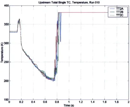
As in all blow-down facilities, a phenomenon known as compressional heating can be observed at the early stage of the startup transient. The high pressure in the supply tank coupled with the initial vacuum in the test section has the effect of compressing the gas and, therefore, heating it, as explained in [5]. This phenomenon is very short in time and its duration is directly linked to the speed with which the valve opens. So far, only

(47)

fast response probes have been able to detect it. Hence, the capacity of a probe to record this phenomenon, which translates into a temperature spike, as shown in Figure 3.5, is an experimental criterion for a probe response qualification.

Uputrem TohISinde TC, Teraur. Run 010

I Time (9)

Figure 3.5 - Compressional Heating in the Blow-Down Seen by the Upstream Probes. 3.4.2. Upstream and Downstream Total Temperature Single Probes

As is explained in section 3.6.2, an efficient way to reduce the conduction error for a given probe is to expose significant length of wire to the flow, on either side of the junction bead. But this length should also allow the gage wire to sustain the dynamic pressure of the blow-down flow. In these circumstances, it was decided to manufacture

-inch single thermocouple heads.

For these heads, the gage is inserted in a -inch OD casing with a 0.016-inch thick wall. These casings are each vented with two holes diametrically opposed, whose dimensions have been determined by the surrounding flow conditions and the recovery error, as explained in section 3.6.1. The gage wire is hung between two half-inch-long

(48)

wire ends are soldered to 0.010-inch diameter thermocouple extension wires, inside the ceramic tubes. These extension parts run through a 3/16-inch stem tube, filled with epoxy to seal the probe. These single probes are mounted via Swagelock fitting on brass plugs located at the inlet and outlet stations of the compressor. These extension wires connect to thicker thermocouple extension wires to the external ice point reference chambers were they mate with temperature reference junctions maintained at 0*C. The signal is caught there and led to special conditioning instruments that will be described in section 3.4.5.

Figure 3.6 - Downstream Temperature Probe Mounted on Brass Plug. 3.4.3. Upstream and Downstream Total Temperature Rakes

In order to determine the radial distribution of the temperature at the inlet and the outlet of the compressor, total temperature rakes have been designed. They consist of specially designed airfoils fitted with thermocouple heads on their leading edges. One rake is located upstream of the compressor, it supports 11 heads, spaced in such a manner that they will record temperature figures for similar annular areas. The reduction in the flow duct radius led to the design of two downstream rakes, one with 5 probes and the other with 6 probes. The arrangement of these heads is again organized in a way that all probes will cover identical annular flow areas. However, we should underscore the

(49)

exception of the tip probes on the 6-head rake, that had to be shifted towards the mid-radius of the duct, due to their casing diameter.

These airfoils have been designed so as to disturb as little as possible the flow pattern. On the one hand, this implies that the airfoils should have the smallest thickness possible. But on the other hand, the thermocouple probe performances are still subjected to conduction error, which require, to be overcome, a larger head diameter. In these circumstances, a consensual approach was found with 3/16-inch head probes. These heads have the same length and share the same layout as their single counterparts, only with a smaller inner casing diameter and a different vent hole size. Each airfoil actually consists of a main body encompassing the leading and trailing edges, with a cavity in the middle, and a cover side sliding in the airfoil span direction. It has a circular base through which it is screwed to an aluminum canister. For manufacturing reasons, each canister consists of two mating parts. The extension wires are laced together at the back of the probe heads and run down the canister to a sealed multi-pin connector where these wires are soldered to thicker thermocouple extension wires crimped to thermocouple grade sockets. The sealing of the connector is ensured by an O-ring placed between the connector part and the aft canister, and by epoxy potting, poured between the sockets. Each of these assemblies fit on machined brass plugs, which mount on the test rig. The downstream rakes have the ability to be rotated with respect to the brass plug, in order for the probes to face the flow and record the total parameters. These orientations are dependent on the speed regime the compressor is tested at. Cables have been made to be mate with the multi-pin connector and connect the thermocouple heads to their external reference junctions, as in the case of the single probe heads. From there on, the information is led to special signal conditioning devices before being recorded by the

(50)

Figure 3.7 - Fully assembled upstream total temperature rake.

Each probe is given an instrument name, according to a certain logic pattern. These names all start by the letters 'TCK', which stand for type-K thermocouples. The following letter can either be an 'R', for the heads mounted on rakes, or an 'S', for the single probes. These letters are followed by a 'U', for the upstream probes or a 'D' the downstream probes. Finally, a three-digit number is added. This information is stored in an electronic instrument database, where each probe is recorded, with the references and names of all the cables and the devices that are active in their functioning. This is not only important for archiving purposes, but also and above all, for calibration purposes, as will be explained in section 3.5.

3.4.4. Mechanical Integrity within the Flow Conditions

After having determined a design capable of satisfying the requirements for the blow-down testing thermal conditions, it was necessary to set up a test that would validate this design in terms of structural integrity of the probes when they are submitted to the dynamic pressure of the flow. In this purpose, a free-jet stand was used. This facility consists of a plenum tube with a circular opening at one end and a connection to a pressurized air system at the other. The gas expands isentropically through the open exit of the plenum. The total pressure of the gas is hence conserved. Inside the plenum, the speed of the gas is close to zero. It is hence possible to monitor the dynamic pressure

(51)

coming out of the plenum tube by setting its inner pressure to a certain value through a feeding valve. Pa Pt Plenum Thermocouple Head

Figure 3.8 - Schematic of Free Jet Resistance Test.

To gather the best efficiency out of this validation test, the simulation aimed at reproducing the strongest dynamic pressure the probes were likely to encounter in the compressor. These conditions occur for the design speed test, at the downstream locations, at the starting of the transient blow-down. The dynamic pressure reaches almost 6 psi in such conditions. The pressure inside the plenum had to be brought to

20.7 psi to reproduce these conditions, and to achieve a safety factor of one. The probes

were than exposed to this dynamic pressure in different ways. The first way tried to systematically search for the pressure leading to the gage break. A given probe would be submitted to any total pressure values between the ambient pressure and the limit value of 22 psi, in steps of 0.5 psi. Several tests showed that the downstream probes were unable to sustain the level of dynamic pressure required. Many broke just around 21 psi, which was perfectly suitable for the upstream probes, which would only be submitted to total pressures of 18 psi at most. Digital camera pictures showed that the breaking points were systematically located at the nearest proximity of the bead junction. The manufacturing process requires the two thermoelectric metal wires to be at a 60' angle from one another, at the location where the bead is machined. Our probe manufacturing process required stretching this gage, creating elbows in the immediate vicinity of the bead. Kinking the gage wire in this location turned out to render it more fragile.