2-loop perturbative invariants of lens spaces and a test of Chern-Simons quantum field theory

2-loop Perturbative Invariants of Lens Spaces and

a Test of Chern-Simons Quantum Field Theory

by

Richard Stone

B.Sc. (Hons.) Australian National University (1990)

Submitted to the Department of Mathematics

in partial fulfillment of the requirements for the degree of

Doctor of Philosophy in Mathematics

at the

MASSACHUSETTS INSTITUTE OF TECHNOLOGY

June 1996

©

Massachusetts Institute of Technology 1996. All rights reserved.

Author ... ...

. .

· · · · · ·· · · ·...

Department of Mathematics

May 23, 1996

Certified

by...,

.... .

.r.,I .... ../,. .r . ... .. . . ..

Scott Axelrod and Isadore Singer

Professors of Mathematics

Thesis Supervisors

Accepted

by....-.

...

Chairman, Departmental

:'

: SiA6Ci,'Sr

r...e

ei

`

a'rs

.'1'

is

-OF TECHNOLOGY

JUL 0 8 1996

David A. Vogan

Committee on Graduate Students

2-loop Perturbative Invariants of Lens Spaces

and a Test of Chern-Simons Quantum Field Theory

by

Richard Stone

Submitted to the Department of Mathematics on May 23, 1996, in partial fulfillment of the

requirements for the degree of Doctor of Philosophy in Mathematics

Abstract

We calculate the 2-loop invariants of a one-parameter family of lens spaces, L[p], as defined by Axelrod-Singer's perturbation theory for the SU(2) Chern-Simons action around the trivial connection. We show that our values agree with those expected on the basis of the sub-leading asymptotics of the exact Witten-TQFT solution for the partition function of Chern-Simons quantum field theory. This extends, for the first time beyond the semi-classical setting to higher loops, existing "experimental" tests of the validity of the path integral defining the partition function and of Witten's "exact," physics-based analysis of it. In doing so, it verifies consistency, at least to two loops for these spaces, between the exact and perturbative treatments of Chern-Simons quantum field theory, and provides the first non-trivial evaluations of higher-loop invariants for the Axelrod-Singer theory.

A key element in the working is the derivation of a completely explicit form of the propagator for the theory on S3. This should be an important ingredient in any future effort to undertake the theoretically important evaluation of all the higher-loop invariants of S3. Certain integral identities concerning this propagator which arise in our evaluation of the Lp] 2-loop invariants may also be useful in any such effort. Thesis Supervisors: Scott Axelrod and Isadore Singer

Acknowledgements

I would like to express my gratitude to the many people whose friendship and support have been so important to me during my time at MIT. Within the mathe-matics department I think especially of Kirsten Bremke, Giuseppe Castellaci, Radu Constantinescu, Peter Dodds, Bruce Fischer, Gustavo Granja, Colin Ingalls, Edith Mooers, Peter Trapa, Chris Woodward, Dan Zanger and Dana Pascovici, but also of many others over the last five years. I think also of many people outside the de-partment, among whom I would like particularly to single out Alan Blair, Andrew Hassell, Veronika Requat, Alice Carlberger, John Matz, Serena Keswani, Diane Ho, Tom Lee and above all Papa Rao.

To my parents and family I owe more than I can express for their unfailing love and understanding.

But most of all I would like to thank my joint thesis advisors, Professors Scott Axelrod and Is Singer, without whose interest, patience, and mathematical guidance, especially on the several occasions when I feared I had encountered insurmountable difficulties, this thesis would not have been possible. I feel very fortunate to have obtained my Ph.D. under their supervision.

Contents

1 Introduction and Background

1.1 Background ...

1.2 Sketch of Chern-Simons Quantum Field Theory and Axelrod-Singer's work.

1.2.1 The Semi-Classical Limit ...

1.2.2 Going Beyond the Semi-Classical Setting 1.2.3 The Perturbative Theory ...

1.3 Outline of Thesis ... 1.3.1 The Precise Goal ... 1.3.2 Organisation ...

2 The 2-loop Invariant in detail and Some Computational ies

2.1 Precise Definition of I2°nn(M3_{, Atriv,}

o)

2.1.1 The Graphical piece. 2.1.2 The Counterterm.

2.1.3 A final expression for I2°""(M 3,

2.2 Preliminaries on S3 and Lens Spaces 2.2.1 Coordinates ... 2.2.2 Group Structure. 2.2.3 Lens spaces. .. . . . . .. Atriv, r . . . . . . . . . . . .

Preliminar-,...o.o.... ... o...,... ) . . . . ... .o... ... e... ... 11 11 14 15 16 17 22 22 23 26 26 27 30 30 31 31 33 37

...

...

...

...

...

...

3 Computation of the Propagator

3.1 Initial Reduction of the Computation ...

3.2 Computing the Green's form G(x, y) of A on S3

3.2.1 Computing G0,3(x, y)

3.2.2 Computing Gl,2(x, y)

3.2.3 Computing G2,1(x, y)

3.2.4 Summary ... 3.3 Computing the Green's form

3.3.1 Computing Lo,2(x, y) 3.3.2 Computing Ll,1(x,y) 3.3.3 Computing L2,o(X, y) 3.3.4 Summary ...

on S

3

_...

on S3 ... and G3,o(x,y) on S3 L(x, y) of d on S3 on S3 ... on S3 ... on S ...

3.4 Computing the Green's Form of d on the Lens Spaces Lp]

Graphical Term

Initial Simplifications ... Evaluation of J(k, m, n) ... Evaluation of J2(k, m, n) ...

Singularity Structure and Regularisation . .

An explicit formula for IA (q, p) ... An explicit formula for IB(k, n, p) ... The Final Evaluation of Inn(L[p], Atri,, g)

5 The Counterterm, the Full 2_{-loop Invariants,}

the Exact TQFT Solution

5.1 Evaluation of CSg,.av,,,(g, o) on L[p] ...

5.2 Final Computation of

and Comparison with

128

. . . 128

I2n (L[p],

Ato, a)

and Comparison with the Exact TQFT Solution ... 130

41 . . . . 41 43 43 46 81 83 84 85 90 93 94 96 4 The 4.1 4.2 4.3 4.4 4.5 4.6 4.7 100 100 105 108 113 118 123 126

Chapter 1

Introduction and Background

1.1 Background

In his paper [W] Witten defined a new class of differential invariants of 3-manifolds, one for each integer k, using Chern-Simons quantum field theory. His invariant,

for each "level" k, is the value of the partition function for the theory, which is a

formal functional integral over the space of all connections (gauge-fields) in the theory. Using physical intuition about the meaning and behaviour of this partition function and deep links with conformal field theory, he was able to evaluate it, and thus to obtain both the values of the invariants exactly for S3, and a "sewing formula" for how the invariants change under surgery on the 3-manifold. Since any 3-manifold can be constructed by surgeries along a set of links in S3, his invariants are thus theoretically calculable for all 3-manifolds. They have now been obtained explicitly in this way for a number of such families of 3-manifolds, chief among them the lens

spaces (see [FG1] and [J1]).

From a mathematician's viewpoint, however, the use of the Feynman functional integral to define the Chern-Simons-Witten invariants is problematic. This is be-cause, despite extensive efforts, a general way of rigorously defining such integrals and justifying the formal properties of them invoked by Witten is still unknown. To a mathematician therefore, it is not apriori clear that his invariants are even

well-defined.

One way of resolving this difficulty is to find an alternative, mathematically rigor-ous definition of them for which the value of the invariants on S3 is the same and for which the same sewing formula can be derived. Such a program has been successfully carried out from two different viewpoints. On the one hand an axiomatic formula-tion of topological quantum field theory (TQFT), encoding the physical insight about the behaviour of the partition function used by Witten without formally introducing functional integrals, has been used by various authors, beginning with Atiyah, to rigorise Witten's invariants. On the other, they have been shown by Walker ([Wall), following work of Kirby and Melvin ([KM]), to arise from a more algebraic theory due to Reshetikhin and Turaev ([RT]) which uses quantum groups to generalise the original work of Jones on knots in S3.

In abandoning Witten's quantum field theoretic starting point, however, neither of these alternatives quite manages to capture the full power of his heuristic Feynman integral approach. For example, by evaluating the semi-classical limit of the partition function using a formal stationary phase argument for the functional integral, Witten was able to obtain a formula giving the asymptotic behaviour of his invariants as k -oo. It is not known how to obtain this formula in either the TQFT or Reshetikhin-Turaev frameworks.

Given this, and the enormous interest of Chern-Simons quantum field theory in its own right, we instead focus in this thesis on a third strategy, due to Axelrod and Singer (also investigated by Kontsevich). This strategy retains the partition function path integral as the centrepiece and attacks the problem of understanding it head on, by showing that in this theory it can be interpreted in a mathematically rigorous way. This is done by approaching the partition function from the point of view of

perturbation theory. Using this they define a different class of "perturbative

Chern-Simons-Witten invariants" whose content should be essentially equivalent to that of the invariants introduced by Witten; i.e. roughly speaking, a knowledge of either set in toto should permit one to pass readily to the other set. In their papers [AS1]

and [AS2] they succeed in proving that these perturbative invariants are rigorously well-defined and give finite, differential invariants of 3-manifolds.

Unfortunately, however, computation in their perturbative framework is consid-erably more difficult than in either Witten's original heuristic approach or the two subsequent alternative formulations of it. Indeed, to date, no calculations of any perturbative invariants for any 3-manifold have been performed, other than the ob-servation, by Axelrod and Singer themselves, that the "even-loop" invariants of S3

vanish identically for trivial symetry reasons. More fundamentally, neither a compu-tation of the full set of perturbative invariants for S3 (i.e. odd loop aswell as even), nor a derivation of the sewing formula have been obtained, and indeed, both tasks currently appear formidable. Thus it remains open as to whether Axelrod-Singer's rigorous perturbative version of Chern-Simons quantum field theory is consistent with Witten's original heuristic version and its later, non-field-theoretic rigorisations.

We note in passing, however, how significant a successful demonstration of this expected consistency would be. For it would not only constitute an index-type the-orem of great importance in 3-manifold theory, relating the purely topological and representation-theoretic TQFT class of invariants to their geometric/analytic pertur-bative counterparts, it would also show that, in Chern-Simons theory at least, the

traditional perturbative treatment of the partition function can be mathematically

made sense of in a way that reproduces Witten's exact solution and so justifies his formal, physics-based working. This would add greatly to the mathematical credibil-ity of quantum field theory and of the functional integral heuristics used routinely in its study both by physicists and, increasingly, by topologists and geometers.

In this thesis, therefore, it is precisely this consistency question with which we are concerned, albeit with a much more modest and experimental goal than proving the desired consistency. Our aim is simply to use the Axelrod-Singer perturbative theory to extend, in a direction that was not previously accessible, the strong computational evidence which already exists to support the validity of Witten's path integral analy-sis. At present this evidence is all in the form of checks of his exact computations, or

rather their rigorous TQFT versions, against his semi-classical asymptotic formula for his invariants in the limit k -+ oo; i.e. for certain classes of 3-manifolds, namely the lens spaces (numerically in [FG1] and exactly in [J1]) and Brieskhorn spheres (only numerically in [FG1]),the Chern-Simons-Witten invariants have been computed in the rigorous TQFT formulations and their asymptotic behaviour found to agree with Witten's path-integral predictions. This amounts to verifying the mathematical va-lidity of the Witten/TQFT solution for the partition function, Zk , to leading order in its expansion as a perturbation series in k, for these classes of 3-manifolds. Roughly speaking our goal in this thesis is then to use the Axelrod-Singer perturbative defini-tion of Zk to extend this computadefini-tional test, in the case of lens spaces, down below the leading term to the sub-leading , or "2-loop", coefficient also. It is not possible

even to attack this question outside the perturbative setting.

To explain more precisely what we mean by all of this we need now to turn from generalities to give a brief mathematical introduction to Chern-Simons quantum field theory and, in particular, Axelrod-Singer's perturbative version.

1.2 Sketch of Chern-Simons Quantum Field

The-ory and Axelrod-Singer's work

We do not attempt here a fully self-contained exposition of these topics. The reader is referred to the original papers, [W] and [AS1],[AS2] for this, and to the general literature for discussion of the perturbation theory framework in which Axelrod and Singer operate. What follows is only the broadest outline necessary for our purposes. The basic data of Chern-Simons quantum field theory consists of a compact, ori-ented, boundaryless 3-manifold, M3, and a choice of compact, simple Lie group G.

We form the trivial G-principal bundle P = M3 _{x G, and from it the associated}

adjoint vector bundle adP = P Xad g determined by the adjoint representation of

G on g. We identify adP with M3_{x g via the canonical trivialisation of P = M}3_{x G.}

using the canonical trivialisation of P to pull back any A E A to an element (which we also denote A) of l (M3; g) and setting

CS(A) = i Tr(A A dA+

-

A A A A) (1.1)

87r2 3

Here "Tr" is some multiple of the Killing form on g which we will tie down in a moment.

This action is invariant under gauge-transformations connected to the identity in the gauge-group 5, but can vary in discrete steps for arbitrary gauge-transformations due to a "winding number" factor arising from r3(G) - Z. We choose the nor-malisation of "Tr" mentioned above precisely so that these steps are "quantised" in increments of 1. In the case of G = SU(N), which is all that will concern us, this makes "Tr" simply the ordinary trace in the standard N -dimensional representation.

This then allows us to formally quantise the theory "at level k ," k E Z, by defining the partition function to be the Feynman integral over gauge orbits

Zk= |/ e2_IrikCS(A)VA

_(1.2)

since now the integrality of k means that the integrand is well-defined on A/5 despite the lack of strict gauge-invariance at the classical level. Note that, without loss of generality, we may restrict our attention to k > 0 since changing k to -k is equivalent simply to reversing the orientation of M3 and thus the sign of CS(A).

1.2.1 The Semi-Classical Limit

The "level" k plays the role here of in real physical theories, and so the semi-classical limit corresponds to considering Zk as k -+ oo. In Witten's heuristic treat-ment of 1.2 this semi-classical limit is evaluated by a formal stationary-phase analysis after introducing first a metric on M3, to perform gauge-fixing to regularise Zk, and then a counterterm to remove the resulting anomalous metric dependence of the so-lution. In the limit k -+ oo, contributions to Zk come only from the stationary fields of the classical Chern-Simons action, i.e. the (gauge-equivalence classes of)

flat connections. Assuming these form a discrete set, Ai}, then Witten obtains an asymptotic formula for Zk as a sum over the Ai, involving certain highly non-trivial geometric and topological invariants of these flat connections - their Chern-Simons

invariants, CS(Ai), their Reidemeister-Ray-Singer torsions, (M3, Ai), and certain

spectral invariants whose metric dependences cancel out.

1.2.2

Going Beyond the Semi-Classical Setting

The rest of Witten's analysis of Zk, outside the asymptotic regime, is, however, inde-pendent of his semi-classical analysis. Rather than try to extend his asymptotic for-mula beyond leading order, he instead shows how to exactly evaluate Zk for any fixed (arbitrary) value of k. He does this, as remarked in section 1.1, by using heuristic properties of the path integral 1.2, later formalised in the rigorous, axiomatic TQFT

treatment.

The perturbative approach to 1.2, by contrast, seeks to build the semi-classical approximation into an expression for Zk as a full perturbation series in the parameter

k; i.e. rather than analyse Zk for each value of k independently, the perturbative

approach treats Zk as a function of k and seeks a series expansion for it around

k = oo, after factoring out the semi-classical piece which represents the leading

term. Such an expression should then yield the asymptotics to arbitrary order of the exact/TQFT Chern-Simons-Witten invariants, Zk, allowing one to relate the exact and perturbative classes of invariants.

The content of these alternative approaches obviously should be equivalent, but the viewpoint is different - Witten's topological invariants are defined as the values of Zk for each k, while the perturbative Chern-Simons-Witten invariants are defined as the coefficients in the perturbation series for Zk.

There is, moreover, one further important difference between the exact/TQFT and perturbative approaches. Witten's treatment obtains invariants Zk depending only on the parameter k. But perturbative theory, as we shall describe in the next section, involves an expansion of the integrand in 1.2 around a fixed choice of stationary

solution, i.e. flat connection. It thus yields, not a single perturbation series, but one for each of our discrete set of flat connections, whose coefficients are topological invariants of M3 together with the flat connection. We denote the perturbation series

for Zk around the flat connection Ai by Zk(M3, Ai). To get from these more refined

invariants to invariants only of M3, which could then be compared with Witten's,

requires adding the series for all the different flat connections.

1.2.3 The Perturbative Theory

Let us now focus on the perturbative theory and discuss it more fully, since it is the basis of all our work in this thesis.

As remarked, we make at the outset a choice of flat connection, say A( °), on M3.

If d(°) is the exterior covariant derivative twisted by A( °), acting on Q*(M3; adP) Q*(M3; g) to form the complex

Q

0

_{(M; adP)}

_d.

_Q

_{l(M3; adP)}

_d(

_2(M

3

_{; adP) d( n}

3

_{(M; adP) ,}

_(1.3)

then, as in [AS1] and [AS2], we shall consider only the case where H1(), the first cohomology group of this complex, vanishes. This is equivalent to assuming that A(°) is isolated up to gauge-transformations, as we have done throughout the discussion so far in taking the moduli space of flat connections to be a discrete set.

We shall not, however, impose the extra assumption in [AS1] and [AS2] that HOA(O) is also zero, since, for all the 3-manifolds we wish to consider, this will not be the case. It has been shown in [FG1] (or alternatively [J1] or [R]) how Witten's semi-classical formula must be adapted to take account of this non-vanishing of Ho(o). We will see that the necessary amendments to Axelrod-Singer's "higher-loop" analysis are also easily made.

To define now the perturbative expansion of 1.2 around A( °), the first step as

always is to make a choice of gauge-fixing (just as was done in the semi-classical analysis of 1.2 in [W]). In [AS1] this is done by introducing a metric, g, on M3 and

working perturbatively around A( °) _{here, our basic space of fields has changed from} being A to being TA(o)A and it is this latter space to which the gauge condition, which cuts out a subspace complementary to TA(o) (gA(O)) in TA(o)4, is applied.

Axelrod and Singer then show that, by introducing the supermanifold TM_, the initial dynamical field and the ghost fields which arise in this BRS approach can all be combined into a single fermionic superfield, A, with respect to which the action appearing in the gauge-fixed path integral for Zk(M3_{, A}( °)_{, g) has a particularly}

sim-ple form. Since, moreover, there is a natural correspondence between superfunctions on TM_ and differential forms on M3_{, they are further able to translate this simple}

form of the gauge-fixed action, Sgf, succinctly back into the more familiar language

of differential forms.

In this language Sgf then splits naturally into a "free" kinetic piece, A A d(°)A and only a single "interaction term" which is cubic in A. Consequently they are able to read off relatively easily the two key ingredients for generating the perturbative expansion, namely (i) the propagator of the theory, and (ii) the types of vertices allowed in building Feynman graphs in the theory, together with their associated Feynman rules.

(i) The propagator, as always, is the "Green's function," i.e. Schwartz kernel of the inverse, of the kinetic operator d( °)_{, but where, as derived in [AS1], the domain} of d(°) has been restricted to the orthogonal complement of its kernel by a Lagrange multiplier condition on the space of fields, A, over which the gauge-fixed path integral occurs, so that discussion of its inverse, and the associated Schwartz kernel, makes sense. We discuss this Hodge-theoretic inverse of d(°) _{in more detail in chapters 2} and 3. For the moment, the only observation we make is that since the new field, A, in Sgf has pieces of all form-degrees in Q*(M3;g) (due to the incorporation of the ghosts along the way) we must take the Schwartz kernel of (d())- 1 _{on all of}

(kerd(°)) C Q*(M3; g), not just on the degree 1 subspace as one might have expected

from the fact that the original dynamical fields before gauge-fixing were elements of

statement that "we need to sum over all particle types before integrating."

(ii) The presence of only the single cubic interaction term means that the theory has only one trivalent vertex, whose Feynman rule involves the structure constants,

fabC, of g (w.r.t. an orthonormal basis of g in the normalisation determined by Tr)

together with the usual imposition of an integration over the spatial variable labelling the vertex.

The translation into the language of differential forms yields, moreover, one further benefit. It leads naturally to a point-splitting regularisation scheme introduced by Axelrod and Singer in [AS1], which, as always in perturbative analysis, is needed to handle the diagonal singularities of the propagator which arise in computing the amplitudes of Feynman diagrams.

With this background in place we can now finally give Axelrod and Singer's per-turbative definition of Zk. It has the standard form of a product of the semi-classical term and the higher-loop series,

Zk(M3, A(°

),

s) ZkSC(M3, A(o

_),

_{s) Zh(M3,}

_{A() )}

_(1.4)

where here s is a choice of framing (i.e. homotopy class of trivialisations of the tangent bundle) of M3 and, as usual, the higher-loop series is defined as a graphical expansion in inverse powers of k + h,

Zk+h(M 3 ,A(°), s) exp (2 ( i( + h))Ac nn(M3A(0)

s))

(1.5)

1=2

Two important issues require further explanation here, however. The first is the shift in parameter from k to k + h in the higher-loop series. Here h is the dual Coxeter number of the group G (h = 2 for SU(2) ). At the moment this is done purely "by hand" in order to obtain agreement with the exact Witten/TQFT solution, where k + h is the natural parameter. A variety of rationales have been given for this, principally in the physics literature (e.g. [ALR]), but also in [AS1]. However no rigorous justification of it is known at present, and so even though we adopt it, it does represent a current gap in our understanding of the perturbation theory.

The second is the graphical expansion in 1.5, which of course requires further discussion to define what is meant by the symbols Iconn(M3, A(, s) giving the

co-efficients. These are in fact precisely the "perturbative Chern-Simons-Witten invari-ants" referred to in section 1.1. In line with standard perturbation theory one's first guess at their definition would be as the sum of the amplitudes of the connected I -loop Feynman diagrams in the theory; these diagrams all being constructed from our single trivalent vertex with no external edges, and their Feynman amplitudes computed using the propagator and the Feynman rules just outlined, along with the point-splitting regularisation scheme just described.

This, however, would leave the Ico°n n metric-dependent, due to anomalies arising from the use of the metric in defining the gauge-fixing, in particular the consequent metric-dependence of the propagator. To get quantities that are pure differential invariants (of M3 together with A(°)), it is necessary therefore to change our definition of icOnn to include "counterterms" that will cancel the metric-dependence. This is a familiar predicament in perturbative quantum field theory. In [W] Witten showed how this could be done to remove the anomalous metric-dependence at the -loop level and so obtain Zs c, by introducing a framing, s, of the manifold and using a counterterm involving the "gravitational" Chern-Simons invariant of the Levi-Civita connection in the framing s. In [AS1] and [AS2] Axelrod and Singer show how Zhl+h

can be handled in a similar fashion using the same framing-dependent gravitational counterterm introduced by Witten. Specifically, they prove that there exist constants fi, > 2, such that

I[on(M3, A(°), s) = Iconn(M3, A(°), g) - PtCSgv(, s) (1.6)

is a rigorously well-defined, finite, differential invariant for each , where I°0nn (M3, A(), g) now refers to the metric-dependent sum of Feynman amplitudes of -loop graphs just discussed. And they compute the value of 2 explicitly and provide heuristic arguments suggesting that /t = 0 for all > 3.

fully make sense of Axelrod-Singer's perturbative definition of Zk. Even so, however, this is not quite the final form of the perturbative definition of Zk that we will use; by considering more detail the role of the framing, s, in 1.4 and 1.5 we will be led to one trivial change which will be slightly better adapted to our purposes.

The framing was introduced to allow us to cancel the metric dependence of the

II (M3°n( , A(), g) and obtain instead the Io""n (M3, A(), s) . At first glance this seems

to be simply replacing one extraneous dependence with another, and certainly it does seem to undermine our hope of obtaining invariants only of M3 itself and A(). In fact, however, this extra framing-dependence of the I"" is not really a problem. This is because both Axelrod-Singer and Witten resolve explicitly in their work how the quantities Zk, ZkS and Iln" vary on changing the choice of (homotopy class of) framing. Thus although the original Chern-Simons-Witten invariants and their per-turbative counterparts in 1.4 and 1.5 are currently dependent on a choice of framing, we know their framing dependence exactly, and this is effectively as good as having invariants only of M3 and A(°) as desired.

Indeed Atiyah has given an alternative, more elegant, way of sidestepping this issue altogether. In [A] he notes that instead of using TM3 and a framing s to define the counterterms above, we could equally work on 2TM3 - TM3 f TM3, which

has a natural Spin(6)-structure, and use a trivialisation of this vector bundle, known as a biframing . Since, in contrast to the case of framings, a canonical biframing of any 3-manifold does exist, defined by having its "signature defect" (see [A], [FG1], or [J1]) zero, we can thus define a differential invariant of M3 and A(O) only, simply by taking the relevant invariant (Zk or If~ln) with counterterm evaluated in the canonical biframing.

We choose to adopt this convention of Atiyah's in this thesis and it is this which necessitates the minor adjustment to Axelrod-Singer's perturbative definition of Zk

mentioned above. This choice is better adapted to our needs in this thesis, however, because it renders easier the comparisons we ultimately have to make with the work in [FG1], [J1], and [R] in the TQFT setting, where this approach is standard and

Chern-Simons-Witten invariants are always given in the canonical biframing.

To be specific now about our adjusted definition of Zk, let the canonical biframing of M3 _{that we will use throughout in defining our invariants, be denoted by a. Then}

our invariants are Zk(M 3, A(°), a), ZC(M3_{, A(), a) and Iconn(M}3_{, A(°), a), and the}

final metric-independent perturbative definition of Zk that we use in place of 1.4 and 1.5 to replace the arbitrary s everywhere by the canonicala, is simply

Zk(M3,A(O), a) ZSC(M3, A(O),) Zk.h (M3, A(°), ) , (1.7)

where

Zhh(M

3

_,

_A()

_exp

(

_i

₍

₊₍

_h))

_{Ionn(M3A(O),))}

_(1.8)

Z+h 2 i

With this definition now in final form we conclude this section, giving an overview of Chern-Simons quantum field theory and especially the work of Axelrod-Singer, with one last observation. It is that in 1.8 the higher loop series clearly has leading expansion

Zk+h = 1 + (27ri) 2 n(M3, A(° )

_,

_{) (k + h)- + O((k + h)-}2_{). (1.9)}

In 1.7 this then explains our remark in section 1.1 that the checks on ZSC(M 3, A( °), a)

in [FG1] and [J1] constitute tests of the path integral against the exact Witten/TQFT solution at leading order, and that our new 2-loop calculations for lens spaces in this thesis represent an extension of these tests to sub-leading order.

We now leave generalities and end this introductory chapter by stating in precise terms the goal and organisation of the remainder of the thesis,

1.3 Outline of Thesis

1.3.1 The Precise Goal

In [J1] Lisa Jeffrey, following up the initial numerical work in [FG1], uses the TQFT 3

closed form of these invariants for the case of lens spaces with G = SU(2). She verifies that they match the leading-order asymptotics of Witten's semi-classical formula as

k -+ oo.

In this thesis we also restrict to G = SU(2) and to lens spaces (in fact, a subclass of lens spaces which we shall define shortly), but we instead compute explicitly the simplest of the perturbative Chern-Simons-Witten invariants in these cases, namely the 2-loop invariants, I2onn, around the trivial flat connection. Our aim, as remarked on several occasions, is then to use these to check agreement between the perturbative and exact TQFT definitions of Zk to sub-leading order in the asymptotics as k -+ oo,

thus extending the experimental semi-classical tests of the path integral undertaken

by Jeffrey.

In stating this program, however, we have glossed over the fact that, as we pointed out earlier, Jeffrey's non-perturbative TQFT invariants do not depend on a choice of flat connection on the base 3-manifold, unlike our perturbative 2-loop invariants,

I2°nn, which are only defined relative to the trivial connection around which our perturbative expansion is being performed. This discrepancy cannot be ignored since the trivial SU(2) principal bundle, P, over a lens space generally has many (gauge-equivalence classes of) flat connections.

Fortunately, however, this difficulty is not serious. This is because Jeffrey herself, in [J21, showed how a trick involving Fourier resummation can be used to decompose her solution asymptotically into contributions from each of the different flat connections. We thus just have to be careful, when comparing our 2-loop invariants with those predicted by the sub-leading asymptotics of the exact/TQFT solution, to base the comparison only on the component of this solution due to the trivial connection.

1.3.2 Organisation

In chapter 2 we quote the exact definition of the 2-loop invariant, I2°nn(M3_{, Atri, a),}

from [AS1] and explain the different terms present. This involves examining the Feyn-man graphs which arise in computing Inn(M 3_{, Atri,, g), and determining formulae}

for their amplitudes, aswell as giving a precise definition of the canonical biframing, a, and the counterterm in which it appears. We end the chapter with a section introduc-ing a variety of geometric objects and results about S3 _{that we will use extensively,} and defining the class of lens spaces whose 2-loop invariants we will calculate.

In chapter 3 we begin this calculation by performing the lengthy computation of the propagator for the perturbative theory on S3, and deducing quickly from it the propagators on our lens spaces. The relevant results are proposition 3.15 and propo-sition 3.16 (or 3.17) respectively. Their derivation involves intensive computations on S3 exploiting symmetries to reduce to a boundary value ODE problem, but, for

those interested in simply passing directly to these key results, their correctness could alternatively be verified after the fact just by checking them against the properties (PL 0)-(PL 3) in [AS1] which uniquely characterise the propagator (after obvious adjustments to take account of the non-vanishing of cohomology in dimensions 0 and

3 in the present case).

In chapter 4 we then use these propagators in our formula from chapter 2 to calculate the graphical components of i2CO"" for our lens spaces. Again this involves intensive computations and simplifications, some dependent on our restriction of the class of lens spaces under consideration. We show that these graphical contributions

are made up of two non-trivial integral terms (proposition 4.9). The first of these we evaluate exactly (proposition 4.10), but for the second we are compelled to turn to numerical computations to obtain insight; these computations indicate very clearly a certain conjectural formula (conjecture 4.11), on the basis of which we then calculate the value of the second integral term exactly. Our final result (proposition 4.12) is that the graphical contributions to I °"'n turn out to be identically zero for all our

lens spaces, due to exact cancellation of these two non-trivial pieces.

In chapter 5 we turn to the counterterm. We compute it easily (proposition 5.1) by invoking a relationship between it and another well-known metric invariant, the eta-invariant of Atiyah-Patodi-Singer, whose value for lens spaces can be found in the literature. In light of our results in chapter 4 this then gives us the full 2-loop

invari-ants, Iconn(M3, Atri,, ) , for our lens spaces with G = SU(2). Having obtained these

we then finally perform the desired comparison between our values and those expected on the basis of the sub-leading asymptotics of the trivial connection contribution to the exact TQFT solution, as extracted from either [J2] or [R]. Our main result in this thesis is that these values agree , providing the further "experimental" support for the validity of the objects and techniques of quantum field theory discussed earlier in this chapter.

Chapter 2

The 2-loop Invariant in detail and

Some Computational Preliminaries

2.1 Precise Definition of

I2onn(M

3

_,

_Atriv,

_a)

Quoting from Corollary 5.6 of [AS1], with a trivial adjustment to accomodate our use of the

canonical biframing rather than the arbitrary framing s, the 2-loop invariant

I2conn(M3, Atriv, o) is defined by

Co(M3 Atriv, ) = 2 on(M 3, Atriv, g)-

48

2rav ).

CSgrav(, ). (2.1)

(

We refer to I27Cnn(M3, Atriv,,g) as the graphical piece of this formula, and

h dim(G) ~ as th

48 CSgrav(g, u) as the counterterm. Note that we are using here that Axelrod-Singer's formula for the 2-loop invariant, obtained in the acyclic setting in [AS1], needs no amendment at all to take account of non-vanishing Ho. This fact is remarked upon in [AS1] (section 6, part II, remark (i)), with an unpublished proof by Axelrod (personal communication).

2.1.1

The. Graphical piece

As defined in chapter 1, I'conn(M3, Atriv, g) is the sum of the Feynman amplitudes

of the connected vacuum-vacuum 2-loop graphs in the theory, evaluated using the propagator and the Feynman rules, which incorporate Axelrod-Singer's point-splitting regularisation.

Since we only have a single trivalent vertex in the theory there are precisely two such graphs, the well-known dumbbell graph and sunset graph (for those unfamiliar with these terms, see [AS1] where they are depicted explicitly). We now discuss them in turn.

Let us consider the sunset graph first. An expression for its amplitude, Isunset, has already been computed in the explicit formula in equation (5.89) of [AS1]. Note, however, that in quoting this formula we will be implicitly adopting, as we shall throughout the remainder of the thesis to facilitate easy reference, two conventions from [AS1] that need remark. The first is the obvious notational convention of dis-tinguishing a particular copy of M3, and objects associated with it, by adding the

name of a variable parametrizing that copy as a subscript. The second, however, is the very unusual policy (adopted to be compatible with their superspace conven-tions) of equipping M.3 x M3 with the non-standard orientation so that the positive volume form is volMy A volM3 not volM3 A volM3. In order to retain the identity

fM3XM3 = fM3 fM3 ,this in turn necessitates choosing the sign convention that

/M3[O

(y)

A X(X)] -[JM (y)] (X) for X E Q*(M 3) and f E Q3(My), (2.2)

which is the opposite of the usual one, and means that the exterior derivative operator,

dx, anticommutes with M3 rather than commuting.

With these conventions, the promised formula for Isun,,et from [AS1] is

Isunset = 1-

J33

falblc fa2b2C2 Lala2(x, y) A Lblb2(x, y) A L1C2(x, Y) (2.3)

Here the fabC are the structure constants of g with respect to an orthonormal basis

{Ta

}, i.e. [Ta, Tb] = fabCTc, and the Lab(X, y) are copies of the propagator, which, from

its definition as the Green's form of dAri, on Q*(M3; adP), is a differential form on the

product space M3 x My with value at (x,y) in Hom((adP)y; (adP)x) . The a,b indices in Lab(X, y) denote matrix indices on using the isomorphism Hom((adP)y; (adP)x) -gz g y (discussed in detail shortly) to write the value of the propagator at (x, y)

as a matrix with respect to the T. Finally, we are, of course, using, as we shall for the remainder of the thesis, the Einstein summation convention of summing over repeated indices.

Equation 2.3 for Isunset can, however, be further simplified. This is because in

[AS1] it has been derived for an arbitrary flat connection and group G, whereas we are dealing only with the simplest possible flat connection, Atriv, and G = SU(2). To see how this makes matters easier let us focus first on the propagator.

As discussed in chapter 1, this is the Hodge-theoretic Green's form for the exterior

covariant derivative, dAtriv, on Q*(M3; adP). To understand it better we start by

describing the action of dAtriv on Q*(M3; adP) more concretely.

Let s: M3 -+ P: x - (x, e) be the canonical trivialisation of P and use it

together with the {Ta} to trivialise adP by sections a,: M3 -+ adP: x -+ [(x), Ta]. Then, since is globally horizontal with respect to Atri, on P, it follows that if we write a general element, v, of Q*(M3_{; adP) in the form va®s.a with each va E Q*(M3),}

the action of dAtri becomes simply the action of the ordinary exterior derivative d

on the coefficient forms; i.e.

dA,, (V) = (dva)

0

Sa (2.4)

But the trivialisation of adP via and the {Ta} that we have used here to get 2.4 is precisely just the standard identification of adP with M3 _{x g that we referred to} at the beginning of section 1.2 and have used frequently already. In particular it is exactly the identification that we used above in 2.3 in writing the propagator as a matrix-valued form.

It thus follows immediately from 2.4 that for Atriv this matrix form of the propa-gator simplifies greatly, splitting globally into a tensor product of spatial and matrix

pieces

Lab(, y) = L(x, y) 0 Sab (2.5)

where the spatial piece , L(x, y), is the Hodge-theoretic Green's form of just the ordinary exterior derivative d on Q*(M3), and the matrix component, dab, is simply

the Kronecker delta symbol.

Substituting this back into 2.3 then gives the first simplification promised in our expression for Isunset, due to specialisation to the case of Atriv, namely

sunset = 12 xM falblL fa2b2C' a la2 6blb2 6c lc2 L(x, y) A L(x, y) A L(x, y) . (2.6)

The final simplification then comes from the specialisation to G = SU(2). For, with the inner product on su(2) discussed in Section 1.2, it is easily seen that its structure constants with respect to an orthonormal basis are given by

fabc = V'fab . (2.7)

In 2.6, our final expression for Isunset in our setting thus reduces to simply

Isunset =

1/

3

L(x, y) A L(, y) A L(x, y), (2.8)

xM

with the group-theoretic pieces having been calculated out of the integrand.

As for the other graph, the dumbbell, for a general flat connection its amplitude is not zero. But once again, for the trivial flat connection we are using, the situation simplifies and its Feynman amplitude is identically zero.

This is because the point-splitting regularisation we use, described in detail in [AS1], involves an antisymmetrization in the group-theoretic indices in the propaga-tor. In light of the global splitting of the propagator for Atriv in 2.5 and the symmetry of its group-theoretic piece, 6ab, this leads to the regularised propagator being iden-tically zero on the diagonal in M x M3. This immediately forces the integral for

Idumbbell (See [AS1], eq. (5.88)) to vanish.

This then completes our discussion of the graphical piece in 2.1.

2.1.2 The Counterterm

This is easier to describe. To begin with, as noted in Chapter 1, the Coxeter number

h is 2 for G = SU(2) so that hdim(G) = 1 48 8

As for the term CSgrav(g, a), recall from chapter 1 that for this we are working not on TM3, but on 2TM3 _ TM3 _TM 3_{, which we are imbuing with a natural}

Spin(6)-structure using the lifting to Spin(6) of the diagonal embedding: SO(3) - SO(6)

(See [A]). On this vector bundle we now first take the connection given by the direct sum of two copies of the "gravitational" Levi-Civita connection for the metric g on

TM3_{. And secondly we form the canonical biframing, a, defined uniquely by the}

index-theoretic requirement that, for any 4-manifold, Y, making M3 _{its boundary}

we have

1

Sign(Y) = pl (2TY, a) ,

(2.9)

where Sign(Y) is the Hirzebruch signature of Y and pl(2TY, a) is the relative Pontrjagin number of 2TY with respect to the biframing a on the boundary (Again see [A] for more details). Then CSgrv(g, a) refers simply to the Chern-Simons invariant of this connection evaluated in this canonical biframing a.

2.1.3

A final expression for

Inn(M

3

_{, Atriv,}

_c)

We conclude this section now by drawing the discussion in sections 2.1.1 and 2.1.2 together to obtain our final definition of 2cann, simplifying 2.1.

Definition 2.1 The 2-loop invariant I'n(M 3_{, Atriv, a), in the case G = SU(2), is} given by simply

n°

'(Ma, Atri, ) x L(x, y) A L(x, y) A L(x, y) - CSrav(g,7) (2.10)

where L(x, y) is the Hodge-theoretic Green's form of the ordinary exterior derivative

d on fQ*(M3) and CSgr,,(g,a) is as described in section 2.1.2.

The bulk of the remainder of this thesis is then concerned with using this definition

existing tests of the partition function path integral, as discussed in Chapter 1. With this in mind, we end this chapter with a section preparing for these computations. In it we describe various geometric objects and results regarding these spaces that we

will use repeatedly.

2.2 Preliminaries on S

3

_{and Lens Spaces}

Since even our computations for lens spaces will generally be reduced to computations on S3, we start by setting up a variety of different coordinate systems, identifications,

and associations between objects on S3 that we will need. We turn to lens spaces themselves only at the end of the section.

2.2.1

Coordinates

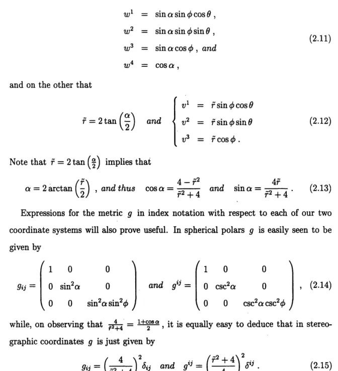
We take standard coordinates on 4 as w, ...., w4 and S3 as the submanifold

{(w, w, 2 W3, W4) I (Wl)2 + (W2)2 + (W3)2 + (W4)2 = 1} , with metric g the standard

.metric induced from 4.

Two sets of coordinates on S3 will be used. The first is standard spherical polars (a, A, 0) ; a E [0, 7r] is the angle down from the "North pole" N = (0, 0, 0, 1) , and for any given ao E (0, r), (, 0) are the standard polar coordinates on the 2-sphere

of radius sin ao obtained by slicing S3 at height w4 = cos ao .

In many ways these are not good coordinates. They are singular at a = 0 and 7r (the North and South poles, N and S), and, for any a E (0, r), at q = 0 and w. Thus

they break down as coordinates on the entire great circle

{(W1_,

w2, w3, w4) E S3 I W1

= W2= 0}. Nonetheless, by taking appropriate care, we

will use them extensively.

The second set of coordinates is stereographic rectangular coordinates on S3 \ S}, obtained by stereographic projection from S onto TNS3 = R3. We denote these

coordinates v1, v2, V3 and define - /(vl) 2 + (v2) 2 + (V3)2.

These are good coordinates on the entire patch S3\ {S}, but they are somewhat

more cumbersome than spherical polars, which is why we often still opt to work in these latter coordinates.

The relationship of these two coordinate systems to each other and to the ambient wi-coordinates can then easily be deduced. We have, on the one hand, that

w

1

_{= sinasin cos8,}

w2 = sinasin sin ,

W3 = sin acos , and

W4 = COS ,

l

(2.11)

and on the other that

r=2tan(-2

V1 and v 2 V3 = rsin q cos 0 = rsin X sin

=

rcos.

Note that = 2 tan (a) implies that

a

=

2 arctan(2) , and thus cos

ci

4

-

_{r_2}

_{4_}

=

2F

+4

and sina=

2 + 4 2 + 4

'

Expressions for the metric g in index notation with respect to each coordinate systems will also prove useful. In spherical polars g is easily

given by 1 0 0 0 sin2_a 0 0 0 sin2a sin2q _J' 1 and gij = 0 0 0 Csc2a 0 0 0 CSC2a CSC2q (2.13) of our two seen to be J , (2.14)

while, on observing that 2 l+ ca= , it is equally easy to deduce that in

stereo-graphic coordinates g is just given by

4

and gi = (2

4

)

2

_i.

gij = 2 + 4 6ij and g = 4 '

4~

)

(2.15)

Note that stereographic projection is conformal.

Finally, from these expressions for the metric we can also write down at once

(2.12)

in each coordinate system. We have that

volS3 = sin2asin d Ado A dO = 2 + 4) dv Adv2_{A d} 3_,

while * is given, in spherical polars, by

*da = sin2a sin d A dO

*do = sin X dO A da

*dO = csc 0 da A do

* (da A do) = sin X dO

* (do A dO) = csc2a

csc

b da , *volS3 = 1,

* (dO A da) = csc do

(2.17)

and in stereographic coordinates by the same formulae for 0 and 3-forms and

*dv

=

(

+2

+ 4)

E jk dvJ A

dvk,

* (dvi A

dv)

= 4) d . (2.18)

2.2.2 Group Structure

We will also use crucially in our computations that S3 has a nat

S3 SU(2)

{

(

EGL 2(C)

l +

Ibl

The explicit identification of S3 with SU(2) that we choose is

ural group structure,

2 =

_.

_(2.19)

S3 3 (WI, 2, W3 W4) ( (W4 + iW3) (WI + iW2) E SU(2). (2.20)

(-w + iw

2

) (w

4

_-

_i

3

₎

This is not, perhaps, the easiest or most natural identification. It has been arranged in this way simply so that the identity element of SU(2) corresponds to the North pole,

N = (0, 0,0,1), while preserving orientation (relative to the standard orientations

on SU(2) and S3). Under it, inversion in SU(2) corresponds to the simple map

(wy 2, U , 4) 1 (-W, -W2, -W3, w4), and even more importantly, the metric g

turns out to be bi-invariant. We will return to this in a moment.

First, however, we use the group structure on S3 to introduce global left-invariant vector fields and dual 1-forms.

33 *1 = vols3,

Definition 2.2 Let {Xi}3=I be the left-invariant vector fields on S3 obtained by defining (Xi)N - w E TNS3 for i = 1, 2, 3 and left-translating, and let {i}3= be the dual left-invariant 1-forms.

Note that our choice here to introduce left-invariant objects in utilising the group

structure of S3 is, of course, arbitrary. We could equally well use the corresponding

right-invariant quantities in everything that follows.

We will use the Xi and i extensively in our calculations because they are globally defined. They thus avoid the singularity problems which arise with the coordinate vector fields and 1-forms in either of our coordinate systems, making computation immeasurably easier.

As elements of the Lie algebra su(2), it is easy to see that the Xi correspond under 2.20 to

0 I 0 i i 0

X

1

=

,

X2 = (

), and

X3=

)

(2.21)

-1 0 i 0 0 -i

and so satisfy the structure relations

[Xi, Xj] = 2ijkXk .

(2.22)

Dually, it then follows from the Maurer-Cartan relations that our left-invariant 1-forms satisfy

d9i = -ijkO A Ok. (2.23)

We would like, now, to relate group-structure and coordinates by expressing these left-invariant objects, Xi and i , in terms of the coordinate systems discussed in the

previous section. Such expressions will frequently prove useful in our computations. They can be obtained by a series of routine, though rather long and tedious, compu-tations. We simply quote the relevant formulae here, leaving their derivations to the reader.

domains where. each of these coordinate systems is well-defined) by

cot a cos 0 cos 8 + sin O cot a cos 0 sin 0

- Cos 6 (- cot a sin 4) ( ( cot 4 cos 6-cot a csc 0 sin cot 4 sin 8+ cot a csc 0 cos 0 -1

(1-4+ 2 )

(-v 3 + 2v V2) (v2 + vlv3) (V3 + 1Vlv2) 4T 2

(-v

2

+ Ivv

3

)

(v

1

+ v

2

v

3

)

(-v1_(-+ 2V1 ₂2V3)

cot a cos 4 cos 8 + sin 8 cot a cos 4 sin 8

- cos 8 (- cot a sin 0) ( ( cot q cos 8-cot a csc 4 sin 8 cot 0 sin 6+ cot a csc 4 cos 8 -1 = (4 _{= 2+}

₄₎

2 (1- 2 v2L2_) (-V3 + 1V1V2) (v2 + 2v1V3) (v3 + vv2)

(1-4+

)2v

)

(-V 1+ 123) (_v2 + lVlV3) (Vi + V2V3) (1 4f + 2 )~ 4 2

This lemma, in turn, then yields as an immediate corollary our important earlier assertion that the metric g is bi-invariant. For equation 2.24 for the Xi, together

35 I \ X1 X2 / (sin cos 8) (sin sin 8) cos 4 ( ( ) )

\

(2.24) I vAl a2.3

and therefore, dually,

, (2.25) ! 'L I \" / ( (sin 4 cos 6) (sin sin ) cos 4 ) / da sin2a do sin2a sin2bdO6 (2.26) / . . dv' dv2 r/.,3 (2.27) r a 1 \ ;,_{\ U} ! I F % V 71 I !

\

\

I

/

\

3 / i 1 I

with 2.14, implies at once that the Xi are orthonormal everywhere on S3 . Thus left-translation preserves the orthonormality of the basis ((9iw)N}=l in TNS 3, which proves the left-invariance of the metric. And identical computations can likewise be performed for the corresponding right-invariant quantities to establish the metric's right-invariance.

Two useful consequences, moreover, then flow directly from this;

i) Since the Xi are orthonormal, so are the i, and so the volume-form and Hodge-star are particularly simple when expressed in terms of the i_{, namely}

vols3 = /1 A 2 A 03 , (2.28)

and

1 = vols3, *.i = ( A 0)(i), *(9 A /)(i) = i, and * vols3 = 1, (2.29)

where, in 2.29, we are adopting, as we shall for the rest of the thesis, the natural cyclic notation of writing

(1 _Oeitj A)_0), ( i)_{- - A i = 1, 2, 3. (2.30)}

ii) For any h E SU(2), the two natural maps of left-translation and right-translation by h are isometries of S3 _{= SU(2). Since the isometry group of}

S3

is S0(4), we can therefore think of them as elements of S0O(4), denoting them by

£h and Rh respectively. We thus have two natural embeddings,

£: SU(2) ,-

S0(4):

h 1_{h , (2.31)}

and

: SU(2)

,

S0(4):

h

Rh

(2.32)

We denote the images of SU(2) inside S0(4) under these embeddings by SU(2)L and SU(2)R. Note that clearly SU(2)L and SU(2)R commute inside SO(4) since left and right translation commute on SU(2).

A quick calculation using the identification 2.20, moreover, gives us these embed-dings explicitly; if h = (wl, w2, w3, w4), then we find that

I , Ch= W4 -w 3 w2 w1 W3 W4 -W 1 w2 and JRh = _W 2 W1 W4 W3 _W1 _W2 _W3 W4 W4 W3 -W 2 W1 -W 3 W4 W1 w2 2 1 _w4 3 _(2.33) 2 1 W 43W _W!-- W2 _W-3 L~~~~~'W4

We shall use these concrete forms of these embeddings crucially at several different steps in our calculations. As a first example, note that they encapsulate the following useful general expressions for the SU(2) product in terms of the ambient coordinates;

Wl

w=

-

WWy

W4W

+ W2Wy

+ WWy,

W

Yw ;+WZW WZW lWZ I Y(2.34)

wy= -wwy+

Wy = -W2y

+

+ WW2

+ ww

W4Wy W3W4

,

and

.and

4

-W

11

22

w33.w

2

33

+

44

Wzy

- -

- - -

WzW

WxWy

--

+W4W

·

We now conclude this section on group structure with one final computational lemma that will also prove extremely useful. It gives the directional derivatives of the ambient-coordinate functions, treated as elements of CO(S3), in the directions of the

Xi vector fields. Again its proof is by direct, if somewhat long, computation (this time applying equations 2.24 for the Xi to equations 2.11 for the ambient coordinates), and so we once more leave the details to the reader.

Lemma 2.4 For i, j E {1, 2,3},i : j, we have

Xi(Wi) = W4 (no sum), Xi(Wj ) = Eijkk, and Xi(w4) = -w i (2.35)

and, as a corollary of the last relation,

X

i

(a)= cscawi .

(2.36)

2.2.3

Lens spaces

We have now introduced all of the geometric structure on S3 that we will use in our computations. The time has finally come to consider the lens spaces whose 2-loop

37 I~~~~~~~~~~~~

invariants we'aim to compute.

For this thesis we do not consider the full phylum of lens spaces (i.e. all L(p, q)

with p, q E Z, as described in, for example, [J1] or [FG1,2]), but rather just a single

species, involving only one integer parameter, p, which are particularly well-adapted to our SU(2) group structure on S3. We denote these by L[p], p > 1. They are

defined as quotient spaces of S3 by the action of a finite cyclic group.

Specifically, take S3 as SU(2) via 2.20, and consider the copy of Z embedded

in the diagonal subgroup, generated by the element

e P 0

Zp ( -2i x (2.37)

0 e

We define the lens space L[p] as the quotient of SU(2) by the left-action of this copy

of Zp; i.e. Lp] SU(2)/Zp with elements being left -cosets Zph, h E SU(2).

Alternatively, we can use the left-embedding in 2.33 to understand L[p] in less group-theoretic terms; namely L[p] is obtained by taking S3 C R4 and gluing together points related by either

/

\

Cl,p -S,p 0 0 Sl,p Cl,p 0 0 Lzp = 0 0 C1,p S,p 0 O -Sl,p Cl,p e S0(4) (2.38)

or any power of Lzp. Here cl,p denotes cos(2) and s,p denotes sin(2).

Remarks and Notation:

(i) These lens spaces are particularly well-adapted to our SU(2) group struc-ture on S3 because the copy of Z by which we are quotienting lies not only as a subgroup inside S0(4) (using such subgroups we can get all lens spaces L(p, q)), but in fact lies in SU(2)L inside SO(4). Hence, for example, all our left-invariant

objects on S3, such as the Xi, i and g, descend naturally to any L[p], where we will continue to denote them by the same symbols.

This last fact provides our first indication of the advantages of restricting our attention to the Lp] family of lens spaces in this thesis. We shall defer a completely

thorough discussion of this issue until chapter 4, however, where we will be better

positioned to explain in full detail our reasons for limiting the class of lens spaces under consideration.

(ii) For reference, we note that in terms of the more standard notation for lens spaces as L(p, q) , our lens spaces Lp] correspond to the spaces L(p,p - 1). This is easy to see from the quotient definition of the L(p, q) given in [FG2] and our characterisation of L[p] using L given in 2.38. We shall need to keep this in mind in chapter 5, when we come to extracting from the literature the exact TQFT predictions for the 2-loop invariants for comparison with our own calculated values. (iii) Although we shall not notationally distinguish between such quantities as

Xi, Oi or g on S3 and down on Lp], it will prove useful to explicitly distinguish points on L[p] from points on S3, in order to avoid confusion between a point on

S3 and the point on Lp] determined by its Z-coset. To this end, we shall adopt a convention of writing points on L[ip] with a "bar" over them; i.e. for any point

x E S3, the "point" Zx E L[p] will be denoted .

Having now defined the lens spaces L[p] and made these remarks, we conclude this section and the chapter by considering one final issue of obvious importance, namely the relationship between the L[p] and 3.

Clearly, from our definition, we have a natural covering map from S3 _{down onto}

L[p]. Denoting this by 7rp, it is then evident that 7r* is an injection from Q*(L[p])

back into *(S3), whose image consists of those forms, , on S3 _{which are invariant} under the left-action of Z, i.e. L£k = j for all k = 0, 1,..., p - 1. Denoting these

p

Zp -invariant forms on S3 by *zp(S3), we can thus define an inverse map

p: Qz(S ) Q*(L[p]) (2.39)

such that p o r = id.