A machine learning approach for digital image restoration

(1)

Student : Calixte Mayoraz Professor : Dominique Genoud

BUSINESS INFORMATION TECHNOLOGY

A MACHINE LEARNING

APPROACH FOR DIGITAL

IMAGE RESTORATION

(2)

Calixte Mayoraz

HES-SO Valais, August 2017 I

FOREWORD

The photography industry has changed drastically in the last few decades. When we used to have film cameras and vacation pictures we wouldn’t see until we returned home and developed them, we now have smartphones that allow us to take near unlimited pictures and preview them instantly. Back then, family photos were taken with the help of a professional photographer. The prints were meticulously saved in albums, labeled, dated, and sorted. Up until the mid 2000s, pictures were always printed, and sometimes, more recently, digitized to adapt to the new internet world. Today, these tables have completely turned around: we instantly share thousands of pictures on social media, and very rarely print them. While some aficionados still romanticize the retro aspect of printed pictures, the smell of a photo album, or the grain from old film; the truth is that these media are not timeless. Indeed, pictures wear, colors fade, albums get torn, and are subject to the elements. Moreover, sharing pictures from an old photo album is impossible to do over large distances, albeit sending the entire album by mail, which is not very practical.

It is with regards to these disadvantages of physical images that many companies start to offer digitizing solutions for older media. These companies do not stop at the digitization of images, but also provide digitization of old video reels, audio tapes, VHS, etc. to ensure an infinite lifespan to these treasures of the past.

This study is conducted in partnership with the Swiss company Cinetis, specializing in this type of digitization, and in the context of a final Bachelor thesis for the HES-SO Valais. The goal is to provide a prototype web application which would accelerate the cropping of individual images within a photo album scan by automatically detecting the images within scans.

This study provides several different approaches to solve image-detection issues, and create a web-based user interface. In addition, many explanations of computer vision concepts, as well as machine learning concepts are explained in depth in this research paper.

(3)

Calixte Mayoraz

HES-SO Valais, August 2017 II

ACKNOWLEDGEMENTS

I wish to thank the following people that supported me throughout this Bachelor thesis and helped make this paper what it is today:

Mr. Dominique Genoud, who proposed the topic and supported me throughout this thesis as well as throughout my entire Bachelor education at the HES-SO Valais.

Mr. Jérôme Treboux, who gave me precious advice as to how to advance the research during frustrating times, and helped greatly with the writing of this paper. His advice and friendship were of great value during my years at HES-SO.

Mr. Jean-Pierre Gehrig, the project owner from Cinetis, who also provided great advice and feedback during our weekly sessions. His enthusiasm in this research and positive reactions to the results were a great motivation.

My father, Nicolas Mayoraz, for his everlasting support, his insight in the field of machine-learning, and help with the writing of this paper in English.

All of my fellow classmates with whom I shared these three years. Our late nights, hard work, and mutual support finally paid off, we did it!

Ms. Milène Fauquex, whose warm company and support made these three years at the HES-SO some of the best in my life.

(4)

Calixte Mayoraz

HES-SO Valais, August 2017 III

FOREWORD'...'I!

ACKNOWLEDGEMENTS'...'II!

TABLE'OF'CONTENTS'...'III!

ABSTRACT'...'6!

STATE'OF'THE'ART'...'7!

DROPBOX'MACHINE'LEARNING'APPROACH'...'7!

PYTHON'EDGE'DETECTION'APPROACH'...'10!

LIMITATIONS'OF'THESE'APPROACHES'...'11!

1.! INTRODUCTION'...'12!

1.1.!

CONTEXT'OF'THE'RESEARCH'...'12!

1.2.!

GOAL'OF'THE'RESEARCH'...'12!

1.3.!

BASIC'CONCEPTS'OF'COMPUTER'VISION'...'12!

1.3.1. !

DEEP!LEARNING!AND!CONVOLUTIONAL!NETWORKS!...!13

!

1.3.2. !

FEATURE!DETECTION!...!13

!

2.! METHODOLOGY'AND'TECHNOLOGIES'...'14!

2.1.!

METHODOLOGY'USED'...'14!

2.2.!

TECHNOLOGIES'USED'...'14!

2.2.1. !

MACHINE!LEARNING!...!14

!

2.2.2. !

PYTHON!...!14

!

LIBRARIES!...!15

!

2.2.3. !

PHP!/!JAVASCRIPT!...!15

!

LIBRARIES!AND!FRAMEWORK!...!15

!

3.! CHOICE'OF'APPROACH'...'15!

3.1.!

MACHINEBLEARNING'BASED'...'16!

3.1.1. !

RANDOM!FOREST!...!16

!

(5)

Calixte Mayoraz

HES-SO Valais, August 2017 IV

IMAGE!PROCESSING!CONCEPTS!...!16

!

PREAPROCESSING!AND!GROUND!TRUTH!...!17

!

TRAINING!AND!TESTING!...!19

!

LIMITATIONS!OF!THIS!METHOD!...!21

!

3.1.2. !

NEURAL!NETWORK!...!21

!

PREAPROCESSING!...!22

!

GROUND!TRUTH!...!24

!

MODELING!...!25

!

3.2.!

FEATUREBDETECTION'BASED'...'26!

3.2.1. !

HOUGH!TRANSFORM!...!26

!

HOUGH!TRANSFORM!EXPLANATION!...!28

!

ISOLATING!RECTANGLES!...!29

!

LIMITATIONS!OF!THIS!METHOD!...!30

!

3.2.2. !

CONTOUR!FILTERING!...!31

!

MORPHOLOGICAL!TRANSFORMATIONS!...!33

!

CONNECTED!COMPONENT!ANALYSIS!...!35

!

SIMPLIFYING!SIMILAR!RECTANGLES!...!37

!

4.! IMPLEMENTING'THE'USER'INTERFACE'...'39!

4.1.!

WEB'SERVICE'...'40!

4.1.1. !

CONSIDERED!APPROACHES!...!40

!

4.1.2. !

REST!WEB!SERVICE!...!41

!

4.2.!

WEB'PLATFORM'...'41!

4.3.!

JAVASCRIPT'EDITOR'...'42!

4.3.1. !

CREATING!DIFFERENT!TOOLS!...!42

!

4.3.2. !

RESIZING!RECTANGLES!USING!LINEAR!ALGEBRA!...!44

!

5.! RESULTS'...'45!

5.1.!

COMPARING'THE'METHODS'...'46!

5.2.!

ROOM'FOR'OPTIMISATION'...'46!

(6)

Calixte Mayoraz

HES-SO Valais, August 2017 V

5.2.1. !

OPTIMIZING!THE!FEATURE!DETECTION!APPROACH!...!46

!

5.2.2. !

OPTIMIZING!THE!UI!...!47

!

5.2.3. !

OPTIMIZING!THE!RANDOM!FOREST!APPROACH!...!47

!

5.2.4. !

OPTIMIZING!THE!NEURAL!NETWORK!APPROACH!...!48

!

5.2.5. !

OPTIMIZING!THE!HOUGH!TRANSFORM!APPROACH!...!48

!

6.! CONCLUSION'...'49'

6.1.!

FUTURE'WORKS'...'49!

SWORN'STATEMENT'...'50!

LIST'OF'FIGURES'...'51!

WORKS'CITED'...'53!

(7)

Calixte Mayoraz

HES-SO Valais, August 2017 6

ABSTRACT

This paper illustrates the process of image restoration in the sense of detecting images within a scanned document such as a photo album or scrapbook. The primary use case of this research is to accelerate the cropping process for the employees of Cinetis, a company based in Martigny, Switzerland that specializes in the digitalization of old media formats.

In this paper, we will first summarize the state of the art in this field of research. This will include explanations of various techniques and algorithms involved with feature and document detection used by various digital companies. We will then introduce our study with an in depth explanation of several computer vision algorithms. The next chapter will explain which technologies were used in the development of the prototype, and which management approach we used to conduct this research. We will then explain four different approaches that were executed to obtain results in image detection. This chapter will include detailed methodology and explanations of each step of each approach. The four approaches demonstrated in this paper are a Random-Forest based approach, a Neural-Network based approach, a Hough-Transform based approach, and a Contour-Filtering based approach. The first three did not yield good enough results and were not used in the final version of the prototype. The Contour-Filtering approach however, proved to be very efficient and was used in the final prototype. The next chapter will explain how the retained approach was used to implement a user interface for the prototype application. The final results will then be measured and explained, and possible optimization options will be discussed. This section will lead to the conclusion of this study and future works that could be derived from the prototype.

(8)

Calixte Mayoraz

STATE OF THE ART

Existing mobile applications already exist to scan photo albums, the most popular one being Photomyne (Photomyne, s.d.). This app allows the user to quickly scan photos from a photo album by taking a picture with a smartphone. However, no blog, documentation, or paper has been published by Photomyne developers explaining the inner-workings of their application.

While searching for published works on this type of problem, we quickly noticed a distinction in nomenclature. Most of the work pertaining to edge-detection or photo detection, most of the work pertaining to these search terms were focused on detecting the edges within an image, such as the Canny edge detection filter (Canny, 1986). It quickly became clear that the works more adapted to our problem were oriented towards document detection rather than edge detection.

Two published works in particular were at the heart of the inspiration of this study. The first was found in the Dropbox tech blog (Xiong, 2016) and the second was explained in a python tutorial to build a simple document scanner (Rosenbrock, 2014).

DROPBOX MACHINE LEARNING APPROACH

In the first work, Xiong explains the process that Dropbox uses to scan documents in their mobile app. The app has a camera that surrounds the document in the image in a blue rectangle in real time. Once the user takes the picture, the framed document is then cropped and transformed to fit in a rectangle. This image is then converted to PDF format and stored on the user’s Dropbox account. A screenshot of the app in action can be seen in Figure 1.

(9)

Calixte Mayoraz

Figure 1 - Dropbox document scanner surrounding the detected document with a blue frame. Source : (Xiong, 2016)

This technique focused on a process that needed to be simple enough to be calculated on a handheld device in real time at 15 images per second. The entire process explained in this article can be broken down into four parts: edge-detection, computation of lines from an edge map, computation of intersections, and isolation of the best quadrilateral. Xiong defends the use of machine-learning as being more efficient than traditional edge detection to detect “where humans annotate the most significant edges and object boundaries” (Xiong, 2016).

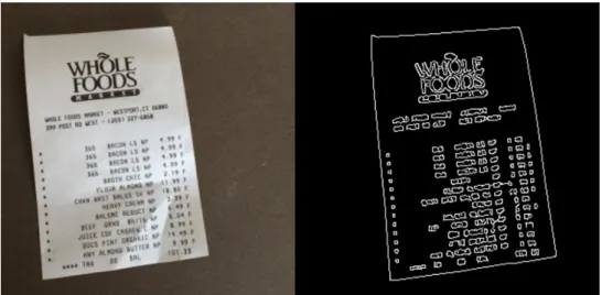
In the first step of his process, Xiong explains the drawback of using traditional edge-detection algorithms such as the Canny edge detection filter. He explains that “the main problem is that the sections of text inside the document are strongly amplified, whereas the document edges—what we’re interested in—show up very weakly” (Xiong, 2016).

To overcome this obstacle, Xiong trained a random-forest model to recognize pixels that were on a border based on annotated images with interesting borders highlighted by humans. Mapping the probability of each pixel being on an edge provides an “edge map” of the image giving a much clearer view of the borders that are interesting to the scanner as seen in Figure 2.

(10)

Calixte Mayoraz

Figure 2 - Canny edge detection, left. Edge map of random forest, right. Source: (Xiong, 2016)

Once the edge map is computed, the app still needs to isolate straight lines. Indeed, we have a pixel image that contains the lines visible to the human eye, but the actual equations of those lines still need to be computed to be interpreted by a program. To determine lines from this image, Xiong uses a Hough Transform. This mathematical transformation converts lines into points, plotting the slope and offset coordinates of the line on the x and y axes of the new mathematical space. A more detailed view of how this transformation works will be explained in Section 3.2.1. The resulting image is a plot of the lines represented as points. In this view, the lighter spots of the plot indicate lines in the edge map computed by the random forest model. A visualization of this plot can be seen in Figure 3.

Figure 3 - Edge map, left. Edge map after Hough Transform with lighter points emphasized, right. Source: (Xiong, 2016)

(11)

Calixte Mayoraz

The local maxima detected in the Hough Transform plot can now be transcribed as lines. For example, a maximum located at (150, 1) on the Hough Transform plot has the equation:

! = 150& + 1

From there, it is easy to plot all detected lines onto the original image to obtain Figure 4.

Figure 4 - Detected lines plotted over source image. Source: (Xiong, 2016)

At this point, all that is left to do is isolate all the four sided polygons from these lines. Each polygon is given a score depending on the probability of its edges being actual edges from the edge map in Figure 2. Finally, the polygon with the highest score is selected. At this point, the app has the coordinates of the document the user is most probably trying to scan, resulting in the preview in Figure 1.

PYTHON EDGE DETECTION APPROACH

The second work provides a different approach to the problem with no machine-learning. Interestingly, the results from this technique are much more promising than the first one. This work is separated in three steps: edge-detection, contour filtering, and applying a perspective transform. The main idea behind this technique is that instead of using machine-learning to isolate the “interesting edges” we can isolate only the interesting contours from a Canny edge detection, i.e. only the rectangles, as potential candidates of images within a scan. This assumption turned out to simplify the problem considerably.

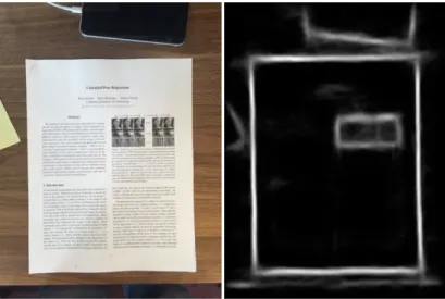
The first step of this process is to apply a Canny edge detection over the image. This will isolate all the edges from the image, and inevitably also isolate the edge the user is actually trying to isolate. The result of this edge detection can be seen in Figure 5,

(12)

Calixte Mayoraz

Figure 5 - Original image, left. Image after Canny edge detection, right. Source: (Rosenbrock, 2014) Once the edge detection is performed, the script iterates over each contour. A contour is defined as a series of adjacent pixels, and is easily detectable using the Python computer vision library OpenCV2 which will be presented in greater detail in Section 2.2.2. Once the script finds the largest contour with four edges, it is assumed that this contour is that of the document the user is trying to scan. From there, the coordinates of the angles can easily be isolated, resulting in Figure 6.

Figure 6 - Source image with detected contour in green. Source: (Rosenbrock, 2014)

LIMITATIONS OF THESE APPROACHES

Both of these approaches work very well to detect a single document that the user wishes to scan. However, they do not offer the possibility to isolate several images simultaneously within a scan. This constraint poses several issues. For example, in the Dropbox approach, the app only selects

(13)

Calixte Mayoraz

the single quadrilateral with the highest score. But what if there are several images to be detected? Which polygons represent what the user wishes to scan? Similarly, in the Python edge detection approach, only the largest polygon is selected. What if several images exist? How do we know which of these large rectangles are actually images we are trying to detect or simply artifacts of the images’ actual content? These questions form the cornerstone of this study.

1.!INTRODUCTION

1.1.! CONTEXT OF THE RESEARCH

This study was conducted to help the Swiss company Cinetis, specialized in digitizing of older media. Currently, when a photo album is scanned, each image is individually cropped using Adobe Photoshop. Although this process can be accelerated by an experienced employee, the repetitive nature of this task begs for automation.

Cinetis required an algorithm that could extract the coordinates of the four corners of each image within a photo album scan. The user would then be presented with a simple web-based interface to select the images, adjust the angles if needed, add new rectangles if some images were not correctly detected, and validate the coordinates. Based on these point coordinates, the cropping can then be done separately and automatically.

Making a web-based prototype frees Cinetis from OS restrictions. The process could even be done on a tablet or smartphone for an improved user experience.

1.2.! GOAL OF THE RESEARCH

The proposed solution would be a PHP web platform where the user starts by selecting the scan to work on. A web-service-oriented Python script could take a filename as input, and return a JSON object containing the coordinates of the four corners for each of the detected images within the scan. The user will be presented with a JavaScript-based editor to view, edit, add, delete, and validate the detected rectangles. Once the user validates the cropping points, a form containing the coordinates in JSON format can be sent to the Cinetis servers for cropping.

1.3.! BASIC CONCEPTS OF COMPUTER VISION

In its broadest sense, image recognition uses a myriad of technologies and algorithms to extract information from images. We often talk about deep learning and neural networks being able to classify images, extract text from an image (Geitgey, 2016), or track motion (Rosebrock, 2015) when

(14)

Calixte Mayoraz

we talk about image detection. In the most conclusive approach of this study, we focused on a type of detection called feature detection. This process isolates geometrical properties from an image and filters the ones that are most “interesting” for the desired result.

1.3.1.!

Deep learning and convolutional networks

Neural networks, more precisely deep-learning and convolutional networks, are particularly good at image classification. Models can be trained to classify objects, people, cars, letters and numbers, etc. In the case of convolutional neural networks, the models can even recognize different objects within a complex image (Geitgey, 2016). In our case, a neural network can be used to recognize the pictures in the scanned album or scrapbook. However, due to the complex nature of neural networks, and the time restriction to complete this study, we decided not to use this type of method. We did, however, attempt to use neural networks to distinguish the corners of each image within a scan. The full development of this approach is explained in section 3.1.2.

1.3.2.!

Feature detection

Feature detection is widely used in computer vision to extract interesting information from an image. For example: edge detection algorithms can help find sudden color changes, connected component analysis can find groups of pixels of the same color and can even calculate the shape of these groups, and Hough transforms can not only to detect straight lines within an image, but also circles. This last algorithm can be used for example to find the vanishing point in the perspective lines of a building as seen in Figure 7 (OpenCV, 2017).

Figure 7 - Using the Hough transform to find the vanishing point of an image. Source: (OpenCV, 2017) The final result of this study uses these tools rather than machine learning to successfully identify images within a scanned photo album.

(15)

Calixte Mayoraz

2.!METHODOLOGY AND TECHNOLOGIES

2.1.! METHODOLOGY USED

The goal of this study being a prototype for Cinetis to use, we worked very closely with their correspondent, Jean-Pierre Gehrig, all along the project. We followed an agile methodology, meeting every week for an hour, presenting the progress of the study, and deciding where the study would go from there. This turned out to be very effective to bounce off of approaches that were too complicated or wouldn’t yield interesting results fast enough.

2.2.! TECHNOLOGIES USED

2.2.1.!

Machine Learning

The first approach of this study was machine-learning based. The data-mining software KNIME is ideal for the initial prototyping of the machine-learning process, allowing quick turnaround in exploration of various ideas before transcribing the workflow in Python.

Due to its graphical node-based layout, see Figure 8, KNIME allows us to quickly manipulate data, train and test various machine-learning models, and analyze the results rapidly. KNIME also includes Python nodes. These nodes allowed for an easier manipulation of the data and would also ease the transition of rewriting the workflow entirely in Python. Several approaches to the study are modeled in KNIME and will be discussed in greater detail in Section 3.1.

Figure 8 - Example of a part of a KNIME workflow

2.2.2.!

Python

We chose to use JetBrains PyCharm Community Edition for the Python development. The ease of use of this IDE, embedded terminal window, along with our previous experience with JetBrains IDEs made it the prime choice to develop the Python scripts.

(16)

Calixte Mayoraz

Libraries(

Python has many libraries to accomplish various tasks without having to reinvent the wheel for every task. The main libraries we used are OpenCV (OpenCV Team, 2017) and NumPy (Numpy developers, 2017).

NumPy is a python library providing efficient implementations of a wide range of complex mathematical functions. The library includes functions for basic statistics, linear algebra, and basic arithmetic over large arrays and matrices.

OpenCV is an image manipulation library with many basic functions like crop, threshold, blur, sharpen, etc. along with more complex feature detection functions like Hough transform, connected component analysis, contour approximation, etc. These features are heavily exploited in this study, significantly reducing the complexity of the Python script

2.2.3.!

PHP / JavaScript

We decided to use JetBrains PHPStorm for the PHP code. From our experience, this IDE was an obvious choice, in part for its ability to parse PHP and JavaScript syntax.

Libraries(and(Framework(

To code the user interface, we used the JavaScript library Paper.js (Lehni & Puckey, 2011). This library’s native use of layers, paths, selection, and editing tools greatly accelerated the user-experience development process.

The general layout of the web-platform was coded using the Yii2 framework (Yii Software LLC, 2017). Having already used this framework for previous works, we were already familiar with the workflow and were able to quickly setup a prototype once the Python script was ready.

3.!CHOICE OF APPROACH

As stated in the state of the art, two main approaches to the problem are tested: a machine-learning based approach, and a feature-detection based approach. In this chapter we will explain in detail how each of these approaches are developed. In the next chapter, we will analyze all the results to defend our final choice of approach for this study.

(17)

Calixte Mayoraz

3.1.! MACHINE-LEARNING BASED

3.1.1.!

Random Forest

In his explanation of Dropbox’ document scanner (Xiong, 2016), Xiong argues that using a machine-learning model to determine an image’s edge map can be used to find the “interesting” edges within an image with more accuracy than traditional edge-detection algorithms. More precisely, he uses a random-forest algorithm to determine each pixel’s probability of being on an edge. The resulting image is an edge map where lines can easily be seen as in Figure 9.

Figure 9 - Left, the raw image. Right, the edge map after random forest. Source: (Xiong, 2016) Having no other information on this algorithm, like which input parameters Xiong uses, we decided to test several options for ourselves to see which results were the most promising.

Image(processing(concepts(

A grayscale image is can be represented as a two-dimensional matrix with values ranging from 0 to 255 (if the image is encoded using 8-bit integers). We can represent a simple 5x5 matrix with random integer values

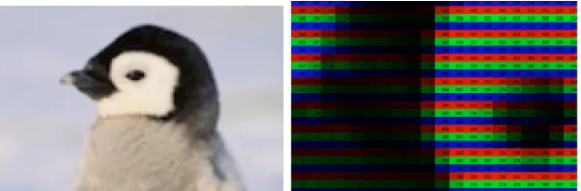
between 0 and 255 as a 5x5 pixel grayscale image as in Figure 10. For an RGB image, the principle is the same, except that we now have to visualize a three-dimensional matrix, with each 8-bit integer encoding one

of three colors: red, green, and blue, as visualized in a spreadsheet with color encoding in

Figure 11 thanks to the ThinkMaths online pixel spreadsheet converter. (Steckles, Hover, & Taylor, s.d.)

(18)

Calixte Mayoraz

Figure 10 - Example of a 5x5 grayscale matrix with random pixel values

Figure 11 - An RGB image of a penguin encoded in a spreadsheet. Source: (Steckles, Hover, & Taylor, s.d.) Pre6processing(and(ground(truth(

For our use-case, we work in grayscale in order to reduce calculation time by a factor of three. To convert an image from RGB to grayscale, a simple average of the three RGB values gives us the overall lightness of the pixel. For the exploration of the solution, we also scale the image down by a factor of 100. The calculation time is too important for the full resolution images which are 6012x9700 pixels large. We are left with a 60x97 matrix with values ranging between 0 and 255 corresponding to a grayscale and scaled down copy of the original as seen in Figure 12.

Figure 12 – A portion of the grayscale matrix, left. The resulting heat map, right.

We now need a ground-truth to determine if each pixel is indeed on a border or not. To accomplish this, we manually create images of the same dimensions as the source images with white frames on the borders’ positions as seen in Figure 13.

(19)

Calixte Mayoraz

Figure 13 - Original image, original resolution, left. Ground truth, original resolution, right.

Each pixel now contains four pieces of information: its X and Y coordinates, pixel value, and ground truth. To increase accuracy, we extract more information from each pixel: its neighboring values. For a first iteration, we collect each pixel’s 24 neighbors in a 5x5 square around it as shown in Figure 14.

Figure 14 – Current pixel’s 24 neighbors

We independently read each image and its corresponding ground-truth image and merge the two tables once the matrices are unraveled, or reshaped as one-dimensional arrays, as seen in Figure 15. Each row in the table represents one pixel. The first two columns represent the X and Y coordinates of the pixel, the third column represents the pixel’s average RGB value, the fourth column represents the ground truth which can either be “Border” or “No_Border” and the next 24 columns represent the pixel’s 24 neighboring values in order.

(20)

Calixte Mayoraz

Figure 15 - Unraveled image matrix with ground truth and neighbors Training(and(testing(

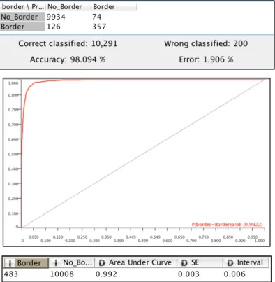
Our data can now be modeled in a Random-Forest algorithm to determine each pixel’s probability of being on a border depending on its position, value, and neighboring values. However, at our first attempt, the classifying algorithm simply classified everything as being “No_Border”. This is due to the ratio of border to no-border pixels being very small. Indeed, in our 18 train images, only 4.6% of the pixels are borders. Using this logic, the classifying algorithm classified everything as being “No_Border” and boasted a 95.4% success rate. To counter this, we use a technique called “bootstrap sampling” to train the model. This technique is used to balance out categories that have very different counts to “trick” the classifier into thinking there are more data points in the less frequent class than there actually are. Training the model in this way leads to much more accurate results with a 98.094% success rate with a standard error of 0.3%. The confusion matrix, ROC curve, and standard error for the predictions can be seen in Figure 16.

(21)

Calixte Mayoraz

Figure 16 - Confusion matrix of random-forest algorithm, top. The ROC curve of the model, middle. Standard error and interval of the ROC curve, bottom

This random-forest model is trained on a concatenation of 18 unraveled image matrices with their 24 neighbors. We can now apply this model to a new image that the predictor had not yet seen. To determine the accuracy of this algorithm, we plot the probability of each pixel being on a border in an edge map as explained in the Dropbox tech blog (Xiong, 2016). The resulting image can be seen compared to the original downscaled image in Figure 17.

Figure 17 - Downscaled image, left. Edge map, right

We can see the algorithm getting close to the desired result that Xiong obtained in Figure 9. To gain precision, we trained another random forest model to predict a pixel’s probability of being

(22)

Calixte Mayoraz

on an edge given its 99 neighbors in a 10x10 square surrounding it. Interestingly enough, adding more neighboring pixels did no significant increase to the algorithm’s accuracy as seen in Figure 18. If anything, the additional data added more uncertainty to the classification.

Figure 18 - Edge map given 99 neighbors around each pixel Limitations(of(this(method(

It is very important to note that at this point, we are working with very low resolution images. When trying to increase resolution to get more detailed edge maps, the computation time increases dramatically. At 10% resolution, the workflow takes several hours to unravel the 18 test images and get all the neighboring pixel values in a single matrix. Moreover, the sheer quantity of the data makes the KNIME environment run out of heap space when trying to train the model. Indeed, 18 images at 600x970 pixels makes over 10 million lines to train. To try to bypass this last constraint, the model was run on a very powerful calculation server of the HES-SO, but the time to execute was still too important. Although the initial results of this process were promising, and further optimization of the code could have accelerated it, we decided to try different approaches to this study.

3.1.2.!

Neural Network

Instead of calculating each pixel’s probability of being on an edge, we tried a different approach which involved training a neural network to recognize image corners. The idea is to detect all the potential corners in the image and use the neural network to classify these potential corners into two classes: “Corner” and “No_Corner”. When all true corners are identified, we can then determine which four corners define the desired image based on where the user clicked. An illustration of this process can be seen in Figure 19.

(23)

Calixte Mayoraz

Figure 19 - Illustration of the process detecting lines and corners, and determining the image based on user click position

Pre6processing(

The first part of this method consists in isolating all potential corners of the image. Our approach is based on the assumption that a vertical or horizontal line can be detected with sudden changes in the sums of pixel rows or columns. To illustrate this assumption in an example, we can imagine the scan having mostly a light-colored paper, the sum of a column of pixels entirely on the paper would yield a very large value due to all the white pixels having a value close to 255. As soon as we examine a column of pixels that contain an image, the sum of the column diminishes, as the image in the scan is inevitably darker than the background paper.

To accomplish this edge detection, we make two copies of the scan, and transform them both into one-dimensional arrays containing the sum of rows and columns respectively. For a 6012x9700 image, this gives us two arrays: a 6012 long array containing the sum of each pixel row, and a 9700 long array containing the sum of each pixel column. We now look at groups of 10 neighboring rows or columns and perform a “sliding window” over all rows and columns and examine the difference between the minimum and maximum of each group of 10 and record this value. Plotting all the pixel-differences for each group shows us clearly the drastic color changes in the scan, and therefore where

(24)

Calixte Mayoraz

the edges of images are. A graphical representation of the lag columns’ min-max difference layered on the original image can be seen in Figure 20.

Figure 20 - Displaying row and column pixel differences

We notice that some color strips in Figure 20 are wider than others. This is due to the fact that some of the images aren’t perfectly aligned and therefore causing the difference of overall color change to be wider than if it were perfectly aligned to the scan. To overcome this issue, we simplify the color band’s coordinate to it’s central value. Therefore, a 25px wide color band spanning from columns 1500 to 1525 would equate to a color change at the X position 1512.5.

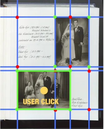
We now have a list of X and Y coordinates where image borders occur. Of course, there is some noise in this data due to the nature of the images. For example, in Figure 20, we see a blue vertical band being detected in the middle of the bottom image. This is due to the subjects in the image having very contrasting clothes and standing close to each other in a near-vertical fashion. When we combine all possible combinations of X and Y, we are left with all potential corners of the image as depicted by green dots in Figure 21. All that remains to do is crop a 100x100px image around each potential corner to be sent to the neural network.

(25)

Calixte Mayoraz

Figure 21 -All possible corners detected in the image Ground(truth(

To obtain the ground truth for all these potential corners, we manually create corresponding images of each scan with white dots on each corner as seen in Figure 22.

Figure 22 - Raw image, left. Ground truth, right

From this ground truth image, we perform a connected-component analysis to determine the coordinates of each point. A more in-depth view of connected-component analysis is explained in Section 3.2.2. We now know the coordinates of each dot in our ground truth. To apply this ground truth to the potential corners detected in the previous step, we iterate each potential corner and search our ground truth coordinates to find a close match. If the ground truth coordinates are within the 100x100px window of each potential corner, the corner is marked as a corner. If no ground truth coordinates match the potential corner, it is marked as a non-corner.

(26)

Calixte Mayoraz

Once this process is complete, the data is ready to be fed in a neural network for classification. A look of this data can be seen in Figure 23.

Figure 23 - Example of images with class labels ready to be sent to the neural network Modeling(

We now have data that is ready to be fed in a neural network to classify the images as corners or no-corners. Having done all the pre-processing steps within the KNIME environment, we decided to continue with KNIME to avoid having to learn to use another unfamiliar software such as TensorFlow (Google, 2017). Luckily, the KNIME platform offers a variety of neural network nodes and example workflows to get started. Within these examples, we found a workflow that classifies various celebrity faces based on AlexNet proposed by Krizhevsky in his paper “ImageNet Classification with Deep Convolutional Neural Networks” (Krizhevsky, 2012). We assumed that this neural network, able to be trained to recognize several celebrities, could easily be trained to classify just two types of images. However, the calculation time was unexpectedly long. The network took two hours to train and two hours to test, and it simply classified everything as not a corner. This disappointing result and important calculation time made it impossible to test the algorithm via a trial and error approach. Having limited knowledge about the inner workings of the deep network, and limited time to finish this study, we decided not to pursue this approach any further. It is important to note however that this approach can be very promising given more research. The pre-processing being relatively fast, clocking in at only a few seconds to detect the potential corners for each image, a trained network could detect the true corners in a very rapid manner, and the end-user would be presented the user interface all in a short amount of time. The corner classification could even be

(27)

Calixte Mayoraz

done asynchronously on the Cinetis servers, storing the coordinates of the true corners in JSON files until they are called for use by the user loading the editor page.

3.2.! FEATURE-DETECTION BASED

3.2.1.!

Hough Transform

Pre6processing(

At this point in the research, we started exploring other possible solutions to the problem. We also tried to diverge from KNIME workflows as we noticed much delay in the Python nodes within the workflows. The next two approaches are developed entirely in Python. While experimenting with different image manipulation techniques and edge detection algorithms, we found an edge-detection filter that could be of use for the project: the Sobel filter (OpenCV dev Team, 2014). This filter is a type of edge-detection filter that can be oriented vertically or horizontally. More precisely, the filter scans for intense color changes given a certain kernel. A kernel is a small matrix, usually 3x3 or 5x5 that defines which pixels the filter will examine when determining if a pixel is on a border. This means that given the right type of kernel, the Sobel filter is well suited for finding vertical and horizontal lines in an image, as seen in Figure 24.

Figure 24 - Example of the applied vertical and horizontal Sobel filters. Source: (OpenCV dev Team, 2014) For our problem, this filter could be particularly well suited to find the edges of the images within the photo album scan.

(28)

Calixte Mayoraz

Figure 25 - Demonstration of the Sobel filter on a photo album scan. Left, original image. Center, Sobel-X. Right, Sobel-Y.

As we can see in Figure 25, the Sobel filter applied to the scan clearly shows the vertical and horizontal lines displayed in the filtered images. At this point, we want to return to the method that Xiong uses in his Dropbox tech blog (Xiong, 2016): use a Hough transform to find the lines in the image and determine possible quadrilaterals from those lines. The Hough Transform requires the image to be in binary form, meaning only pixels with a value of 0 or 1. This is done by applying a threshold to the filtered image. The thresholding process is straightforward: examine each pixel in the image, and compare its value to a given threshold value. If the pixel’s value is equal to or above the threshold value, it is set to 1. If the pixel’s value is below the threshold value, it is set to 0. We are left with a binary image composed of only black and white pixels. The result of applying a threshold to our Sobel-filtered images can be seen in Figure 26.

(29)

Calixte Mayoraz

Figure 26 - Thresholding of Sobel-filtered images Hough(transform(explanation(

With a binary image, we can now apply a Hough transform. As mentioned in Section 1.3.2, the Hough transform is a mathematical transformation capable of detecting straight lines within a binary image (OpenCV, 2017). It works as follows:

1.! Pick a white pixel in the image. 2.! Draw a line going through that pixel.

3.! Count how many white pixels intersect that line, this corresponds to the line’s score. 4.! Calculate scores for every possible line through that pixel.

5.! Repeat for each white pixel in the image.

Once this process is done, we have a collection of lines with scores. The higher the score, the higher the number of white pixels going through the line, therefore, the higher the chance that it is actually a line within the image. The built-in Hough transform function in OpenCV allows us to put a threshold on the score of the lines, so only lines with at least a certain amount of white pixels going through them are kept. Moreover, we know the polar coordinates of each of the retained lines, which means that we know the angle at which they are drawn, allowing us to isolate near-verticals and near-horizontals. When we apply this process to our thresholded image, we get the result seen in Figure 27

(30)

Calixte Mayoraz

Figure 27 - Hough transform applied to the thresholded images.

As we can see, many lines are detected as a result of the Hough transform. This is due to the fact that the lines we wish to detect in our thresholded image are thicker than 1px. The thicker the line, the more possible mathematical lines can correspond to it. An example of this is shown in Figure 28. As we can see, the thick line segment allows many red lines to be drawn within it and have a high enough score to be considered actual lines.

Figure 28 - Many lines passing through a thick line segment

At a first glance, the fact that there are so many lines should not be a problem since it reinforces the assumption that the correct line is indeed there somewhere. However, we will see in the next section that this factor greatly increases calculation time.

Isolating(rectangles(

The next step in this process is to isolate all the potential rectangles that could correspond to the actual images. After identifying all potential candidates, we can use machine learning to determine which of these rectangles are the ones we are looking for. To do this, we first recapitulate the data we currently have and what we are looking for:

(31)

Calixte Mayoraz

•! We have a collection of vertical and horizontal lines •! The images must be of a minimal width and length •! The images can’t be too large

•! The images can’t be too close to the edges of the scan •! We assume the images have a maximal aspect ratio of 2:1

Based on these assumptions, we then couple vertical and horizontal lines in potential couples. These couples should not be too close nor too far away from each other. Once we have a collection of vertical and horizontal couples, we couple each of those couples together to get potential rectangles while keeping in mind the maximal aspect ratio. However, due to the important number of lines detected by the Hough transform, the number of couples grows, and the number of quadruples grows even more, resulting in a very important calculation time. In Figure 29 we can see the terminal output of the calculation of rectangles within the image in Figure 27. We can see a very large amount of potential rectangles found, and an impressive 6-minute calculation time.

Figure 29 - Terminal output of the Python script finding potential rectangles Limitations(of(this(method(

We can already see that to find all the potential rectangles in an image, the calculation hikes up to 6 minutes per image. This important duration spanning only at the pre-processing step, we can only imagine what the total time to find the true rectangles using machine learning would be. In hindsight, using the edge detection algorithm used in Section 3.1.2 would have greatly accelerated this pre-processing step. We could have isolated all potential rectangles much faster, and used machine learning to identify the true rectangles within the image, although the parameters of this

(32)

Calixte Mayoraz

machine-learning process would be subject to further research. Fortunately, the next method was both fast and accurate.

3.2.2.!

Contour Filtering

All previous attempts requiring more time and experience than we had to complete this study, we decided to try an approach without involving any machine learning. Indeed, the problem seems simple enough at a first glance: the background paper is light enough to be able to isolate the images, the images are all rectangles that need to be cut out, there must be a simple answer to detect rectangles within an image. It is with this mindset that we started out on the fourth and final variant to solve this problem.

Pre6processing(

Up to now, the main drawback in our approaches is that the information within the images themselves keeps throwing off our algorithms. To reduce the amount of noise in the image while conserving the most important color changes, we use a median filter. This filter is different than a simple Gaussian blur in the sense that it preserves the edges while smoothing color in an image (Fisher R. , Perkins, Walker, & Wolfart, 2004). We then simplify the scans’ data by using simple brightness and contrast adjustments. After testing on Adobe Photoshop, we found the ideal brightness contrast adjustments to bring out the images as much as possible against the background paper as we can see in Figure 30.

Figure 30 - album scan after median filter and brightness contrast adjust

The scan (still in grayscale mode) can be resumed to a plot to find patterns in its brightness. If we plot the pixel value between 0 and 255 on the x-axis, and the count of pixels having that value in the image on the y-axis, we obtain a histogram of the image. This can be very useful to determine

(33)

Calixte Mayoraz

where to put a threshold to isolate the elements of the image we want. In our case, we plotted histograms for the image before and after color correction. The resulting plots can be seen in Figure 31. When observing the histograms, it is important to note the logarithmic y-scale to get a better sense of the pixel density for each value.

Figure 31 - Images and corresponding histograms before and after color correction

In the histogram of the uncorrected image, we see a few local maxima, but no discernable pattern or visible point at which a global threshold could isolate all the images within the scan without getting noise from the background paper. In the color-corrected histogram however, we observe a very large number of near-black pixels. This is useful because we know that the images in the color-corrected scan are very dark, and we can hypothesize that most of the images will fall within these values. We can also observe the local maxima being more distinctly pronounced at approximately 45, 115, 170, and 240.

We ran an extensive amount of tests to determine the ideal threshold point. The conclusion of these tests is that an optimal threshold for one scan may not be the best for other scans. To make up for this difficulty, we simply sweep the threshold value between 0 and 255 to be certain to catch

(34)

Calixte Mayoraz

all of the images no matter the scan. More precisely, we execute a loop with a counter value that increments 25 times by a factor of 10. Several iterations of thresholding can be seen in Figure 32.

Figure 32 - Thresholding the scan at a value of 1,left. Thresholding at a value of 131, middle. Thresholding at a value of 191, right

At each iteration, we apply the threshold, and perform morphological transformations to close holes and open points. The detail of how these operations work are explained in the next section.

Morphological(transformations(

Morphological transformations are operated on binary images and require two inputs: the original image, and a kernel, which defines the nature of the operation. The kernel is generally a matrix of certain dimensions filled with ones. A more in depth description of these morphological transformations can be found in the OpenCV documentation website (OpenCV dev team, 2014).

Erosion(

Erosion is much like its name implies: it erodes the edges off of contours. This makes all of the contours thinner and removes altogether very small contours. This is useful to reduce noise. However, any holes that occur within contours are accentuated. An illustration of erosion can be seen in Figure 33.

(35)

Calixte Mayoraz

Figure 33 - Original image, left. Eroded image, right. Source: (OpenCV dev team, 2014)

Dilation(

Dilation is the inverse of erosion: it inflates all the contours in the image. Potential holes in contours can be filled using dilation. Inversely to erosion, where holes are accentuated, potential noise on the outside of the contour is accentuated using dilation. An illustration of dilation can be seen in Figure 34.

Figure 34 - Original image, left. Dilated image, right. Source: (OpenCV dev team, 2014)

Opening(

We can notice a pattern occurring. Erosion and dilation both have caveats: they accentuate holes or noise in an image. To counter this, we can use a combination of the two. If we erode the image, noise is reduced and holes are accentuated. However, if we dilate the image after eroding it, the noise is still gone and cannot reappear, but the holes return to their original size. This process is known as opening the image. An example of this process can be seen in Figure 35.

(36)

Calixte Mayoraz

Figure 35 - Original image, left. Opened image, right. Source: (OpenCV dev team, 2014)

Closing(

Inversely to opening, closing allows us to close holes within contours by dilation, and revert any external noise to its original size by erosion afterwards. Holes closed due to dilation cannot be recovered by the following erosion, and information outside the contour is recovered. An illustration of this process can be seen in Figure 36.

Figure 36 - Original image, left. Closed image, right. Source: (OpenCV dev team, 2014)

Of course, due to the geometrical nature of square pixels, information is inevitably lost in each morphological transformation. However, this poses no important problem in our case, since the images we are looking for are very large, and we are not interested in the detailed contours, only the approximate region.

Connected(component(analysis((

Connected component analysis is based on connected component labeling, which will be simplified to CCL in future references. CCL, is a method to detect groups of adjacent pixels of the same color within a binary image. This process works by following a few simple steps:

(37)

Calixte Mayoraz

•! If all four neighbors (or eight depending on the type of CCL you wish to use) are 0, assign a new label to the pixel

•! If one or more neighbors have a value of 1 and no label, assign them and the current pixel a new label

•! If one or more neighbors already have a label, set the label for all of these pixels to the same value.

Once this process is complete, the image will contain an array of connected components and their labels, often displayed in different colors as seen in Figure 37. A complete look at CCL can be found on the Image Processing Learning Resources website (Fisher R. , Perkins, Walker, & Wolfart, 2003).

Figure 37 - Original binary image, left. Image with labeled connected components, right. Source: (Fisher R. , Perkins, Walker, & Wolfart, 2003)

Once we have isolated all connected components in our image, we can perform connected component analysis, simplified to CCA for future reference. CCA will examine each component and determine its centroid, area, perimeter, and various other geometrical properties. OpenCV has many built-in functions to perform useful computations, but the most useful one in our case is the contour approximation function.

Looking at Figure 32, we see that the images isolated by the threshold aren’t perfect rectangles. Their corners are rounded, some edges are rough, and some have holes in them. OpenCV has a function to calculate each component’s contour and, using this function, we could have just isolated all the contours with exactly four edges. However, we would miss most of the isolated images for the very simple reason that they do not appear as perfect rectangles. To solve this, we use the contour approximation function. This function is based on the Douglas-Peucker algorithm (Douglas & Peucker, 1973) and approximates a contour by fitting a contour that is no further than a given value, named epsilon, and get the smallest number of corners possible. This allows us to obtain rectangles from near-rectangles and correctly identify the images in the thresholded binary image.

From here, we perform the same logical operations we did in Section 3.2.1 to further filter out unwanted rectangles. We assume the images are at least of a certain width and height, no taller than ¾ of the scan size (an assumption validated by Cinetis), and that the aspect ratio is no more than 2:1 and no less than 1:2. If all of these conditions are met, we can assume that the contour is that of an

(38)

Calixte Mayoraz

image we are trying to detect. To avoid having rectangles with angles other than 90° (a constraint given to us by Cinetis) we then compute the minimal area rectangle for the contour. This function, also built in OpenCV, finds the smallest possible rectangle containing the contour. The rectangle can be rotated, but all of the angles remain at 90°. Once this entire process is done, we save the rectangle’s coordinates in an array for further filtering.

Simplifying(similar(rectangles(

So far, our process detects the images very well. However, as seen in Figure 38, the program detects most images several times, creating overlapping rectangles. This is due to the fact that we loop the threshold process and save detected images without checking that the image has already been found.

Figure 38 - Output of the program detecting all the images, and some multiple times.

To simplify the similar rectangles into a single one, we start by taking the first rectangle from the array of detected rectangles and copying it to another array of “confirmed” rectangles. As we iterate over the array of all detected rectangles, we compare each of them to each “confirmed” rectangle. If the center of the detected rectangle does not come within 25 pixels of each confirmed rectangle, is is confirmed and copied to the confirmed array. In this fashion, we are left with rectangles that do not share a common center as seen in Figure 39.

(39)

Calixte Mayoraz

Figure 39 - Confirmed rectangles over original image

Some rectangles still remain inside others, however this poses no great issue to the final result, as these rectangles correspond to an image label. On the contrary, it gives the end-user more flexibility on whether he/she wants to include the label in the crop or not.

Looking at the console output in Figure 40, we can see that the process takes under 5 seconds to complete. Furthermore, the majority of this time is spent reading and resizing of the large image file. After a 1/10 resize, the image detection algorithm takes less than a second to detect the images, proving this method’s incredible advantage over the previous ones.

(40)

Calixte Mayoraz

4.!IMPLEMENTING THE USER INTERFACE

We are now ready to implement the user interface of the project. To recapitulate, we now have a Python script that detects the images within a photo album scan and returns the coordinates of these rectangles. Some rectangles are detected twice if they have a frame with a label, and some images still remain undetected. For example, some portraits with very light backgrounds do not generate rectangles in the threshold sweep, and are therefore not detected as images, as seen in Figure 41.

Figure 41 - Portrait on the left not being detected due to the lack of contrast between picture background and the paper

All that remains is to create the user interface for the user to select the correct rectangles, adjust them if needed, and validate the coordinates to crop the images appropriately. Several actors play a part in this process, namely: the user, the web client, the web server, and our Python script. A sequence diagram of the typical user interaction can be seen in Figure 42.

(41)

Calixte Mayoraz

Figure 42 - Web sequence diagram of the user interacting with the system, and the various components of the system interacting with each other.

The user requests a scan to work on, which he/she selects through the web client. The web client sends the requested scan’s filename to the server, which requests the JSON-formatted coordinates of the images within that scan to our Python script. Once the script is executed, the scan and coordinates are sent to the client which displays it to the user in the form of a simple JavaScript editor. The user can then modify the frames using simple tools (select, resize, rotate, add, delete, zoom, pan) and validate the coordinates when satisfied. At this point, we hand over the coordinates to Cinetis for them to crop; our job is done!

4.1.! WEB SERVICE

4.1.1.!

Considered approaches

To provide the user with a web-based graphical interface, we first need a way to get the coordinates of the rectangles to the browser when the user requests it. One option, glossed over in Section 3.1.2, was to have a script continually run to detect the edges of the scans in the background and store JSON files on the server to be instantly ready when the user requests them. This could have been an adaptable solution for our more complex attempts using machine learning which took longer to detect edges, since the user cannot be expected to wait even more than a few seconds for the graphical interface to load. However, thanks to our very fast feature-detection algorithm, we can compute the borders in real time as the user requests them, and return the JSON coordinates less than five seconds later.

(42)

Calixte Mayoraz

4.1.2.!

REST Web Service

Our solution consists of making a very rudimentary REST Web service. Essentially, when the user calls certain functions through a web browser, such as when he/she clicks a link, we can run applications and return the results in various formats. There are five REST function calls, also called verbs: GET, POST, PUT, PATCH, and DELETE. In our case, we simply use the GET verb, essentially saying: “GET me the coordinates of the images within this scan”. Only the filename needs to be sent to the web service, and not the image itself, since the images being already stored on the server. This feature doesn’t slow down the loading of the page.

Making such a rudimentary web service in Python is basic thanks to the web.py library which includes tools to make web services in very few lines of code (Schwartz, s.d.). Our REST function simply takes the filename as input, sends it to the Python script calculating the edges we explained in Section 3.2.2, converts the returned array of rectangles to JSON format, and sends them to the web client. An example output of the web service can be seen in Figure 43.

Figure 43 - Example output of the web service detecting borders of an image

The JSON is formatted as follows: an object named “rectangles” contains an array of objects. Each of these subsequent objects contains four arrays named p1, p2, p3, and p4. Each of these arrays contains two integer values with the x and y coordinates of the point with respect to the resized image. This data can now be easily interpreted in JavaScript to provide a graphical interface for the user to edit the rectangles.

4.2.! WEB PLATFORM

As mentioned in Section 2.2, the web platform was coded using the PHP Framework Yii2 (Yii Software LLC, 2017). This framework allowed fast development of a functional prototype to present to Cinetis. The platform consists of just two pages: the selector page and editor page. The user is first shown the selector page, which contains the filenames of the scans he/she can work on. Once the user clicks one of those links, the browser redirects to the editor page. The editor page contains

(43)

Calixte Mayoraz

a canvas where the JavaScript editor draws the graphical interface to manipulate the rectangles, and then submit the coordinates once he/she is satisfied, see Figure 44.

Figure 44 - The selector page, top, and editor page, bottom.

4.3.! JAVASCRIPT EDITOR

The editor was coded using the Paper.js JavaScript library (Lehni & Puckey, 2011). This library makes use of layers, paths, points, shapes, curves, and event listeners and greatly accelerated the development process of the editor. However, amidst all the features offered within this library, one crucial feature is missing and has to be implemented by hand, resizing rotated rectangles. We explain this feature in greater detail in Section 4.3.2.

4.3.1.!

Creating different tools

First off, the user has to be able to perform several actions on the canvas. Most importantly, he/she has to be able to see the rectangles detected by the Python script, and select those that correspond to actual images within the scan. The first tool is the selection tool, which allows the

(44)

Calixte Mayoraz

user to click on a “guessed” frame, shown as red dotted lines, and “confirm” the rectangle, making it solid green as seen in Figure 45.

Figure 45 - Sections of a guessed image, bottom-left, and confirmed image, top-right.

Using the selection tool, the user can also move the confirmed rectangles, and resize them. Complications in this last step will be discussed in Section 4.3.2. The user can also rotate the rectangles, delete them, add new ones if they aren’t detected as in Figure 41, zoom in and out of the canvas, and pan the canvas to be more precise in the definition of the rectangles. The selection of each tool is done using a simple HTML button interface as seen in Figure 46 which also provides the name of the tool, and simple instructions on how to use it.

(45)

Calixte Mayoraz

4.3.2.!

Resizing rectangles using Linear Algebra

A particularly interesting challenge in the development of this editor is the resizing of the rectangles. Although simple at first glance, the main problem in this feature comes to light with the three following constraints:

•! The angles must always remain 90°

•! The rectangles themselves are not always straight

•! Paper.js considers the rectangles as paths, or groups of points, and not rectangles with width, height, and rotation.

This means that to resize a rectangle by dragging a corner, the two adjacent corners need to be moved as well to conserve all the right angles, and there is no built-in function to simply scale the rectangle like in traditional vector editing software such as Adobe Illustrator. Referring to Figure 47, if the user drags corner C to a new position C’, we know the ∆x and ∆y of that movement. However, we need to calculate the ∆(x’,y’) and ∆(x”, y”) to correctly move the corners B and D and thus conserve all the right angles of the rectangle.

Figure 47 - Representation of the different calculations required to keep all right angles in a scaled rotated rectangle.

(46)

Calixte Mayoraz

The simplest approach to overcome this obstacle is to use orthogonal vector projections. As a reminder, an orthogonal projection is a projection of a source vector onto a destination vector, following the perpendicular of the destination vector. We can imagine the orthogonal projection as the “shadow” of a vector onto another by a flashlight pointed straight down on the destination vector. An illustration of an orthogonal projection is shown in Figure 48.

Figure 48 - Illustration of an orthogonal projection of two vectors v1 and v2 onto the vector w. Source: (Rowland, s.d.)

Indeed, looking at Figure 47, if we apply an orthogonal projection of the vector ((′ onto the vector *+ we obtain the vector ++′. This resulting vector can also be expressed as multiplying a scalar “n” of *+. The orthogonal projection can be rewritten as follows:

,-./₀₁2 ((3 _{= 2 ++′ = 24*+ =}((′ ∙ *+

*+ ∙ *+2×*+

Using this equation, and the fact that we know the coordinates of the points A,D,C, and C’, we can construct all of our vectors and determine ++′, which is the vector by which we need to shift the point D to obtain D’. The same can be applied using the coordinates of A,B, C, and C’ to obtain 77′. Once these vectors are calculated, and the points shifted accordingly, the resizing of the rectangle successfully conserves the right angles of the rectangle regardless of its rotation.

5.!RESULTS

We now have a fully operating web-application that allows users to quickly select images within a scan thanks to a Python script web service. The user can select a scan, have the images within the scan detected in under five seconds, edit them, and validate all within a web browser. Once validated, the coordinates can be sent to any destination in the form of a HTTP POST request. The prototype is now complete and ready to be sent to Cinetis.

(47)

Calixte Mayoraz

5.1.! COMPARING THE METHODS

Looking back on each section of Chapter 3, we demonstrated four different methods to obtain the desired result. Three of them were unsuccessful mainly due to important calculation time and large amounts of data. If more time were given, each of these methods could flourish into their own elegant solutions to this problem, although it is too early to define which of them would be the fastest and most efficient.

For the time being, having only measurable results for the feature detection method, we can only compare execution times for each method so far as seen in Figure 49.

Method Random Forest Neural Network Hough Transform Feature Detection

Calculation time

(per image) 3 minutes 35 seconds 6 minutes 5 seconds

Figure 49 - Table comparing execution times for the four methods

Clearly, the Feature detection method remains in the lead, ahead of the next fastest by 30 seconds. Although, as stated in previous chapters, further optimization and research could bring all of these times down at least to under a minute. As a reminder, in his article on the Dropbox Tech Blog, Xiong manages to run the calculations in real time at 15 images per second using a random forest algorithm (Xiong, 2016). This clearly proves the possibility to optimize these algorithms and bring calculation time down to less than one tenth of a second.

It is mainly based on the execution time and time constraint to complete this research that we decided to keep the Feature Detection method for our prototype and not optimize other methods. The potential of the other methods will be discussed in greater detail in the next section.

5.2.! ROOM FOR OPTIMISATION

5.2.1.!

Optimizing the Feature Detection approach

As stated in Chapter 4 and seen in Figure 41, our algorithm still isn’t at its optimal point. Moreover, this algorithm works well with albums that have a light colored paper as a background. As soon as the background becomes colored or patterned, and is therefore gray when converted to grayscale, the algorithm has a hard time discerning images within the scan. Some images can’t be detected as they are glued too close together on the photo album, and are therefore seen as one big image. This image is rejected in the filtering process as it is “too big” or is not a rectangle. Illustrations of these caveats can be seen in Figure 50.

A machine learning approach for digital image restoration

BUSINESS INFORMATION TECHNOLOGY