Diffusion in periodic, correlated random forcing landscapes

HAL Id: hal-01069753

https://hal.archives-ouvertes.fr/hal-01069753

Submitted on 23 Feb 2016

HAL is a multi-disciplinary open access

archive for the deposit and dissemination of

sci-entific research documents, whether they are

pub-lished or not. The documents may come from

teaching and research institutions in France or

abroad, or from public or private research centers.

L’archive ouverte pluridisciplinaire HAL, est

destinée au dépôt et à la diffusion de documents

scientifiques de niveau recherche, publiés ou non,

émanant des établissements d’enseignement et de

recherche français ou étrangers, des laboratoires

publics ou privés.

Diffusion in periodic, correlated random forcing

landscapes

David S Dean, Shamik Gupta, Gleb Oshanin, Alberto Rosso, Grégory Schehr

To cite this version:

David S Dean, Shamik Gupta, Gleb Oshanin, Alberto Rosso, Grégory Schehr. Diffusion in periodic,

correlated random forcing landscapes. Journal of Physics A: Mathematical and Theoretical, IOP

Publishing, 2014, 47 (37), pp.372001. �10.1088/1751-8113/47/37/372001�. �hal-01069753�

Diffusion in periodic, correlated random

forcing landscapes

David S Dean

, Shamik Gupta

, Gleb Oshanin

,

Alberto Rosso

and Grégory Schehr

1_{Université de Bordeaux and CNRS, Laboratoire d’Ondes et Matière dʼAquitaine} (LOMA), UMR 5798, F 33400 Talence, France

2

Laboratoire de Physique Théorique et Modèles Statistiques (UMR CNRS 8626), Université de Paris Sud, Orsay Cedex, France

3

Sorbonne Universités, UPMC Univ Paris 06, UMR 7600, LPTMC, F 75005 Paris, France

4

CNRS, UMR 7600, Laboratoire de Physique Théorique de la Matière Condensée, F 75005 Paris, France

E mail:shamikg1@gmail.com

Abstract

We study the dynamics of a Brownian particle in a strongly correlated quenched random potential defined as a periodically extended (with period L) finite trajectory of a fractional Brownian motion with arbitrary Hurst exponent

∈

H (0, 1). While the periodicity ensures that the ultimate long time behavior is diffusive, the generalized Sinai potential considered here leads to a strong logarithmic confinement of particle trajectories at intermediate times. These two competing trends lead to dynamical frustration and result in a rich sta-tistical behavior of the diffusion coefficient D_L: although one has the typical valueD_Ltyp∼exp (−βLH)_{, we show via an exact analytical approach that the} positive moments (k>0) scale like〈_D 〉 ∼_{exp [}− ′_{c k L(} β ₎ + _]

Lk H1 (1 H) , and the

negative ones as〈D_L−k〉 ∼exp ( (a k L′ β H 2) )_{, ′c and a′ being numerical} con-stants and β the inverse temperature. These results demonstrate that D_L is strongly non-self-averaging. We further show that the probability distribution of DLhas a log normal left tail and a highly singular, one sided log stable

right tail reminiscent of a Lifshitz singularity.

Keywords: Brownian motion, quenched disorder, anomalous dynamics PACS numbers: 05.40.−a, 02.50.−r, 05.10.Ln

Transport in random media is extensively studied due to its practical and fundamental importance [1 3]. In many cases, the dynamics is modelled as a Langevin process, with a drift generated by a quenched disordered potential. In theoretical analysis, the potential landscape is taken to be either infinitely extended or periodic in space. Stochastic dynamics in a periodic potential, both random and deterministic, is commonly encountered in many different con-texts, including modulated structures [4], superionic conductors [5], colloids in lightfields [6,7], diffusion on regular [8 11] and disordered [12 16] solid surfaces, molecular motors on disordered tracks like DNA/RNA [17 19], and motion in a tilted potential due to a random polymer [20].

Theoretical approaches often assume that the dynamics in a periodic potential reproduces the behavior in an infinitely extended potential. This is implemented by setting the period in thefinal result, e.g. for the velocity (if any) or the diffusion coefficient, to infinity [21,22]. It is crucial to investigate how far such an assumption holds. Especially in the context of numerical simulations carried out for periodic systems, one may ask how reliably their results may be extrapolated to infinite systems.

In this work, we address these fundamental questions for a Langevin dynamics x(t) in a periodic, quenched random potential V x t( ( )) (withV x t( ( )+L)=V x t( ( ))):

η x = − +ξ t V x x t d d d ( ) d ( ), (1)

with η the friction coefficient, ξ t() a Gaussian white noise with zero mean and correlations ξ( ) ( )t ξt′ =2η δT (t− ′t), the overbar being an average over the noise, and the temperatureT is in units of the Boltzmann constant. We consider two cases:

• the ratchet case where V(x) is a fractional Brownian motion (fBm) in time ∈x [0,L], with V (0)=0 and V(L) arbitrary. Thus, V(x) is a Gaussian process with zero mean, 〈V x( )〉 =0, and variance − = − ∈

[

]

whereH∈(0, 1) is the Hurst exponent,V0and l define respectively the typical amplitude

of V(x) and its scale of variation over x. In (2) the angular brackets denote averaging with respect to V(x). Figure1 (left) shows a realization of V(x), with a jump at x = L.

• the translationally invariant case, where V(x) is a stationary Gaussian process, which at short length scales|x−y| ≪Lhas the variance (2), and satisfiesV(0)=V L( ), so that all points are statistically equivalent. The particle in this case diffuses on a ring. A realization of such a V(x) is shown in figure1 (right).

The dynamics (1) involves a combination of two paradigmatic situations: random motion in a periodic potential and the generalized Sinai dynamics in presence of a force

= −

F x( ) d ( ) dV x x that is a time-independent stochastic variable with spatial correlations (except forH=1 2 whenV (x) is the trajectory of a Brownian motion itself so that (1) is the

Figure 1. Sketch of the potential V (x) for the ratchet (left) and the translationally invariant case (right). Here,H=1 3.

logarithmically-confined trajectories, the periodicity of the random potential enforces a long time diffusive behavior with a diffusion coefficient D_L. Here, we show that the trade off between these two competing trends results in a rich statistical behavior of DL. In particular,

DL is strongly non-self-averaging, with both negative and positive moments exhibiting an

anomalous dependence on the temperature, period L and the order of the moment, and being supported by atypical realizations of V (x). For the ratchet case, we obtain exact analytical results, relying on exact bounds, for both positive and negative moments of DL. We also

discuss the full form of the probability distribution of DL, and show that it is characterized by

a log normal left tail and a highly singular log stable right tail, reminiscent of a Lifshitz singularity. We finally highlight the issue of sample to sample fluctuations of D_L. From standard scaling arguments and physical intuition, one expects that our exact results for the ratchet case also hold for the translationally invariant situation, which is harder to analyze analytically. This is confirmed below by thorough numerical simulations [24].

The dynamics (1) in an infinite system for arbitrary H, whereH>1 2 (H<1 2) implies positively (negatively) correlated increments and superdiffusive (subdiffusive) V (x), respec-tively, was discussed in [25] where it was shown thatlimt→∞〈x t2( )〉 ∼ln2H( )t (see also [26]). In contrast, in a periodic system, the long time motion is diffusive for any given realization of the potential V (x), so that we have the diffusion coefficient DL≡limt→∞x t2( ) (2 )t , with DL

given by [27 31] (see also [7,8,12,32])

⎛ ⎝ ⎜ ⎞ ⎠ ⎟

∫

∫

where β is the inverse temperature, and D(0)=T η_{. Clearly, D}

L is a random variable that

fluctuates between realizations of V (x), and has support on[0,D(0)]_{. The inverse of D}

Lmay

be regarded as a product of partition functions in potentials V (x) and −V x( ), respectively. The Brownian version of this quantityfinds applications in disordered systems and has been extensively studied, while our results forH≠1 2 apply to more general situations (note that the marginal case H = 0, when V (X) is log-correlated, was studied in [33]). The expression in equation (3) also describes the ground state energy in a toy model of localization, and its average value was studied in [34] forH=1 2.

Turning to the discussion of the behavior of DL, wefirst reduce the number of

para-meters. In the following, we measure L in units of l [see equation (2)], absorb V0intoβ, and

measure DLin units of D(0), so that DLhas support on[0, 1]5. Now, the typical behavior of DL

is easy to estimate as D_Ltyp∝L2 τ

typ, where the dimensionless L sets the scale of an

inho-mogeneous region, andτtypdefines the typical (dimensionless) time a particle spends in this

region. The random potential V (x) being a fBm, the typical height of the potential barrier over a length L scales like LH, for both the ratchet and the translationally invariant case. Assuming Arrhenius type activation, one expects τ ∼_eβL

typ H , which implies β ∼

(

)

The average behavior of DLis a much more delicate question because, as can be seen from

equation (3), computing the statistics of DLis a highly non-trivial task that involves the study

of an exponential functional of fBm, for which standard methods like the Feynman Kac formula are of little use for H≠1 2.

Let usfirst summarize our main analytical results obtained for the ratchet case: We find that the average of the logarithm of DLis given, to leading order in L, by

5

β

∝ −

D m L

ln L 2 H, (5)

with m= 〈maxs [0,1]∈ V s( )〉. The result in equation (5) is consistent with the logarithmic growth of the disorder averaged mean square displacement in an infinite system:

〈 〉 ∼

→∞ x t t

limt 2( ) ln2H( ), and the argument leading to equation (4). Further on, we obtain sharp bounds for the positive moments(k>0) of the random variableDL:

⩽ ⩽

A Lk( ) DLk B Lk( ), (6)

where, in the limit L→ ∞, the bounds satisfy

⎜ ⎟ ⎜ ⎟ ⎡ ⎣ ⎢ ⎢ ⎛⎝ ⎞⎠ ⎤ ⎦ ⎥ ⎥ ⎡ ⎣ ⎢ ⎢ ⎛⎝ ⎞⎠ ⎤ ⎦ ⎥ ⎥ β β = − + = − + + + + + A L H k C HL B L H k c HL ( ) exp (1 )(2 ) , ( ) exp (1 )( ) , (7) k H H H k H H H 1 1 1 1 1 1

with constants c and C, 0 <c⩽C< ∞, being independent of L, k and β. Both bounds exhibit the same dependence onL k, ,β, from which we infer that the exact asymptotic result has the same functional form. Finally, for the negative moments of DL, wefind

⎛ ⎝ ⎜ ⎞ ⎠ ⎟ β ∼ − D exp a k L 4 , (8) L k 2 2 2 2H

where a is a constant (independent of L k, and β). Our exact results, equations (6) and (8), thus show that the positive and negative moments are dominated by atypical realizations of V (x), in contrast to 〈lnDL〉, see equation (5).

We now turn to a derivation of our results. Using equation (3), the logarithm of DLcan be

formally written as lnDL= lnJ L+( )+ lnJ−( )L +2 lnL, where J L±( ) are stationary

cur-rents through a finite sample of length L with potentials ±V x( ) [26]:

∫

= ±

± −

J L( ) [ Ld exp [x V x( )]]

0

1_{. Statistical properties of these currents for the Sinai}

pro-blem (H=1 2) are known [35 40]. Using the results of [41], and noting that with 〈V x( )〉 =0,J L+( ) andJ−( ) have equal moments, we have for arbitraryL H and to leading

order in L,〈lnJ L+( )〉 = 〈lnJ−( )L 〉 ∝ −m Lβ H, which yields equation (5).

The proof of the result in equation (6) is based on a Theorem due to Monrad and Rootzén [42] on the probability that a fBm V (x), withV (0)=0, remains within a strip of widthϵ for the time x∈[0,L]. DefiningML≡max0⩾ ⩾x L| ( )|V x , the Monrad Rootzén theorem, in our

notation, states thatP M( L⩽ϵ)satisfies

ϵ ϵ ϵ

− − ⩽ ⩽ ⩽ − −

(

)

(

)

(

)

exp H1 L exp H1 , (9)

for0 <ϵ⩽ LH_{, c and C being L-independent constants [see equation (6)].}

Consider the lower bound in equation (6). Suppose we average the positive definite quantity DkLby considering instead of the entire setΩ of all possible paths V (x) only a subset

Ω′ ⊂Ω of paths such thatML ⩽ϵ. This gives the lower bound〈DLk〉Ω ⩾ 〈DLk〉Ω′P M( L⩽ϵ).

However, for paths in Ω′, we have exp ( [ ( )β V x −V y( )])⩽exp (2βϵ), and hence,

∫

∫

ϵ ⩾ − Ω βϵ −

(

)

which holds for any ϵ with0< ϵ⩽ LH_.

The function on the right-hand side (rhs) of equation (10) is a non-monotonic function of ϵ, attaining its maximum at ϵ=ϵ =_{(CL k2}β_H)H +H

opt (1 ). Clearly, the best lower bound

corresponds to the choice ϵ= ϵopt, leading to the lower bound in equation (6). Note that to

satisfy the conditions of validity of the Monrad Rootzén theorem, we require thatϵ ⩽ LH

opt ,

that is,2k Lβ ⩾C H, which is easily realized for sufficiently large L. The derivation of the lower bound is an example of the Lifshitz optimal fluctuation method [43], which has been used to bound the survival probability of particles diffusing in the presence of randomly scattered immobile traps (see, e.g., [44]).

We now discuss the derivation of the upper bound. To this end, we discretize x, and write the rhs of equation (3) as

∫

∫

∑

Given that the fBm starts atV (0)=0, at least one term in the double sum on the rhs takes the value exp (βML), corresponding to the point x = 0 and the point where | ( )|V x attains its

maximal value ML. Now, as all the other terms are positive, we have the bound

β ⩾

−

DL1 exp ( ML), and, thus,

∫

(

)

The integral in the rhs is dominated, for large L, by the small ϵ region, where we can thus use the upper bound in (9). Performing the remaining integral overϵ by the saddle-point method and omitting the pre-exponential terms lead to the upper bound in equation (6). The result in (6) has several striking features. Namely, the function

μ_{( , ,}k β L₎= −ln DL , (13)

k

(as compared to its typical counterpart given by equation (4) as μ ( , ,k β L)∼ k Lβ H

typ ), (a)

grows sub-linearly with k (multifractality), (b) is a non-analytic, sublinear function of β, which implies a rather unusual sub-Arrhenius dependence of the positive moments on the temperature, and (c) exhibits a slower anomalous growth with L as∼L +

H H

1 . This means that the

disorder-averaged DL is generically larger than the one expected on the basis of typical

realizations of the disorder. In turn, this implies that the behavior of the positive moments of DL is supported by atypical realizations of disorder, reminiscent of the so-called Lifshitz

singularities, as discussed above. In conclusion, one cannot infer the dynamical behavior in an infinite system from the positive moments of D_L. This is surprising atfirst glance, as 〈x t2( )〉_is linearly proportional to 〈DL〉, and shows that the limitst→ ∞andL→ ∞do not commute in this system.

The behavior of the negative moments 〈D_L−k〉 with k= 1, 2 ,... is determined by essentially the same approach as above. Note that both the lower and the upper bound onD_L−k are made tighter for a given realization of V (x) by using D_L−k∼exp (k Sβ ), where S is the span of V (x) (the difference between the maximum and minimum) on the interval [0,L]. Therefore, in contrast to the positive moments, the negative moments are supported by realizations of V (x) with a large span. Using the result that for large S,

= ∼ −

P M( L S) exp ( S aL2 2H), with a a constant, integration of equation (12) gives the result announced in equation (8), which displays a super-Arrhenius dependence on the temperature,

a superlinear dependence on k, and a strong dependence on L. A similar result was obtained earlier in [45]. We note that, as for the positive moments, one cannot deduce the behavior in an infinite system from that of negative moments of D_Lin a periodic system, as the latter is supported by atypical realizations of V (x) that have anomalously large span scaling as

∼

S L2H, while the typical behavior isS ∼LH

typ .

Based on our results for the moments, we now obtain the probability distribution P D( L). As already explained, the behavior of the negative moments is supported by anomalously stretched trajectories of V (x) for which the value of DLis small. One may thus expect in view

of the form of the moments in equation (8) that for small DL, P D( L)is log-normal:

⎛ ⎝ ⎜⎜ ⎞ ⎠ ⎟⎟ β β ∼ −

(

)

(

)

To analyze the behavior of P D( L)for DLclose to 1, we recall the formal definition of the

one-sided Lévy distributionν( ),z 0⩽ z< ∞, of orderν (see, e.g., [46]):



∫

The asymptotic behavior of ν( ) is well-known [z 46], and, in particular, one has

ν( )z ∼ z−σ exp (−b zτ) for z→0, where b is a computable constant, σ =(2−ν) (2(1−ν)), and τ=ν (1−ν). It is important to note that this precise asymptotic form is responsible for the stretched-exponential behavior in equation (15), which is immediately verified by substituting the form in equation (15), and performing the integration by the saddle-point method. Moreover, one realizes by making in equation (15) a change of the integration variablez=ln (1 DL) βLH, choosing ν =1 (1+ H), and setting

β =

p k LH_{that equation (15) becomes identical to the result in equation (6), up to numerical}

factors. It follows that for DLclose to 1 (i.e., z close to 0), the distribution function behaves as

⎡ ⎣ ⎤⎦  β β ∼ + −

(

)

(

)

Using the asymptotic ν given above, we get that P D( L) is highly singular near the right

Figure 2.(a) −ln [〈DL〉 L2]versus L for three values of H corresponding to diffusive, subdiffusive, and superdiffusive V (x). The inset shows −〈ln [DL L2]〉as a function of L for three values of H, see equation (5). (b) μ( , ,k β L) in equation (13) as a function of k for L = 512 and three values of H. In all cases, the symbols denote simulation results for the translationally invariant V (x), while the slopes of the solid lines correspond to the results derived for the ratchet case.

We now consider the translationally invariant case. Here, we expect our above analysis, in particular, result (6) to hold, up to possible numerical factors. To demonstrate this, we now present results of extensive numerical simulations: figure 2 for −ln (〈DL〉 L2), −〈ln (DL L2)〉, and μ( , ,k β L), and figure 3(a) for P(lnDL) indeed show a very good

agreement that supports our expectations.

To close, we ask: if we have two different realizations of V (x), and correspondingly, two different values, DLandD′L, of the diffusion coefficient, how likely are these values equal?

We introduce a random variable ≡ _D D₊L_D′ , ∈ [0, 1]

L L

, and analyze its distribution



P ( ) via numerical simulations. Clearly,  = 1 2 maximizing P ( ) implies that the two values of DLare most likely very close to one another. Variables such asplay a key role in

various scale-independent hypothesis testing procedures, in classical problems in statistics, in signal processing (see, e.g., [47]), and in the analysis of chaotic scattering in few-channel systems [48]. Such variables are used to characterize the effective width of narrow dis-tributions possessing moments of arbitrary order [49,50].

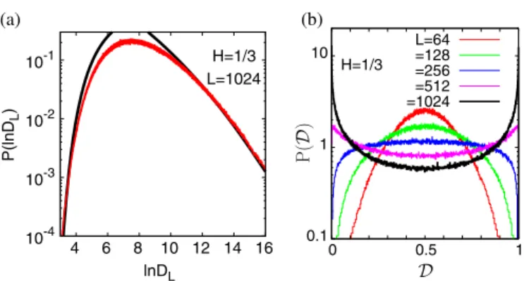
In figure 3(b), we present numerical results for P ( ) for different values of L and =

H 1 3, for the translationally invariant case. We observe an interesting phenomenon of a change in the form of the distribution as L is increased. For relatively small L, the distribution is bell-shaped and centered at = 1 2. However, on increasing L,P ( ) broadens, becomes almostflat at a certain critical L (whose value depends on H), and then changes its shape so that = 1 2minimizes the distribution. This implies that for sufficiently large L, two values of the diffusion coefficients obtained for two different realizations of V (x) are most likely very different, and the eventDL= D′Lis the least probable. Note that a similar dependence in

the distribution of the prefactor in the Sinai law on the strength of disorder was recently observed in [51].

Acknowledgments

GS is supported by the ANR grant 2011-BS04 013-01 WALKMAT. This project is partially supported by the Indo-French Centre for the Promotion of Advanced Research under Project

Figure 3.(a) Distribution P(lnDL) for L = 1024 andH=1 3. The red line denotes numerical results, while analytical predictions for the right and left tails behaving as

−_{a H D}− exp ( ( ) ln H ) L 1 1 _{and exp (−b H( ) ln (D ))} L 2

, respectively, with a(H) and b(H) being constants, are shown by black lines. (b) Numerical results forP ( ) for different

L andH=1 3.

4604 3. SG, AR and GS thank the Galileo Galilei Institute for Theoretical Physics, Florence, Italy for the hospitality and the INFN for partial support during the completion of this work.

References

[1] Bouchaud J P, Comtet A, Georges A and le Doussal P 1990 Ann. Phys.201 285 [2] Bouchaud J P and Georges A 1990 Phys. Rep.195 127

[3] Oshanin G, Burlatsky S F, Moreau M and Gaveau B 1993 Chem. Phys.177 803 [4] Schneider T, Politi A and Sörensen M P 1988 Phys. Rev. A37 948

[5] Dietrich W and Peschel I 1977 Z. Phys. B27 177 [6] Evers F et al 2013 Eur. Phys. J. Spec. Top.222 2995

[7] Dean D S and Touya C 2008 J. Phys. A: Math. Theor.41 335002

[8] Reimann P, van den Broeck C, Linke H, Hänggi P, Rubi J M and Pérez Madrid A 2001 Phys. Rev. Lett. 87 010602

Reimann P, van den Broeck C, Linke H, Hänggi P, Rubi J M and Pérez Madrid A 2002 Phys. Rev. E65 031104

[9] Sancho J M, Lacasta A M, Lindenberg K, Sokolov I M and Romero A H 2004 Phys. Rev. Lett. 92

250601

[10] Lindenberg K, Sancho J M, Lacasta A M and Sokolov I M 2007 Phys. Rev. Lett. 98 020602 [11] Lindner B, Kostur M and Schimansky Geier L 2001 Fluct. Noise Lett. 1 R25

[12] Lindenberg K, Sancho J M, Khoury M and Lacasta A M 2012 Fluct. Noise Lett. 11 1240004 [13] Khoury M, Gleeson J P, Sancho J M, Lacasta A M and Lindenberg K 2009 Phys. Rev. E 80

021123

[14] Reimann P and Eichhorn R 2008 Phys. Rev. Lett. 101 180601

[15] Khoury M, Lacasta A M, Sancho J M and Lindenberg K 2011 Phys. Rev. Lett. 106 090602 [16] Simon M S, Sancho J M and Lindenberg K 2013 Phys. Rev. E 88 062105

[17] Kafri Y and Nelson D R 2005 J. Phys.: Condens. Matter 17 S3871 [18] Kafri Y, Lubensky D K and Nelson D R 2005 Phys. Rev. E 71 041906 [19] Kafri Y, Lubensky D K and Nelson D R 2004 Biophys. J. 86 3373 91 [20] Salgado Garcia R and Maldonado C 2013 Phys. Rev. E 88 062143

Salgado Garcia R arXiv:1404.2852

[21] Derrida B and 1983 J. Stat. Phys. 31 433

[22] Dean D S, Drummond I T and Horgan R R 1997 J. Phys. A: Math. Gen. 30 385 [23] Sinai Ya G 1982 Theor. Probab. Appl. 27 256

[24] Santachiara R, Rosso A and Krauth W 2007 J. Stat. Mech. P02009

[25] Marinari E, Parisi G, Ruelle D and Windey P 1983 Phys. Rev. Lett. 50 1223 [26] Oshanin G, Rosso A and Schehr G 2013 Phys. Rev. Lett. 110 100602 [27] Lifson S and Jackson J L 1962 J. Chem. Phys. 36 2410

[28] Festa R and Galleani dʼAgliano E 1978 Physica A 90 229

[29] Ferrari P A, Goldstein S and Lebowitz J L 1985 Statistical Physics and Dynamical Systems ed J Fritz, A Jaffe and D Szasz (Boston, MA: Birkhauser)

[30] Golden K, Goldstein S and Lebowitz J L 1985 Phys. Rev. Lett. 55 2629 [31] Zwanzig R 1988 Proc. Natl. Acad. Sci. USA 85 2029

[32] Baiesi M, Maes C and Wynants B 2011 Proc. R. Soc. Lond.A 467 2792 [33] Castillo H E and Le Doussal P 2001 Phys. Rev. Lett. 86 4859

[34] Monthus C, Oshanin G, Comtet A and Burlatsky S F 1996 Phys. Rev. E 54 231

[35] Burlatsky S F, Oshanin G, Mogutov A and Moreau M 1992 Phys. Rev. A 45 R6955 [36] Oshanin G, Mogutov A and Moreau M 1993 J. Stat. Phys. 73 379

[37] Monthus C and Comtet A 1994 J. Phys. I France 4 635 [38] Comtet A, Monthus C and Yor M 1998 J. Appl. Probab. 35 255 [39] Oshanin G and Redner S 2009 Eur. Phys. Lett. 85 10008 [40] Oshanin G and Schehr G 2012 Quant. Finance 12 1325 [41] Molchan G M 1999 Commun. Math. Phys. 205 97

[42] Monrad D and Rootzén H 1995 Probab. Theory Relat. Fields 101 173 Li W V, Linde W and Acad C R 1998 Sci. Paris 326 1329

[43] Lifshitz I M 1963 Sov. Phys. JETP 17 1159 Lifshitz I M 1965 Sov. Phys. Usp. 7 549

[44] Grassberger P and Procaccia I 1983 J. Chem. Phys. 77 6281 [45] Comtet A and Dean D S 1998 J. Phys. A: Math. Gen. 31 8595

[46] Schehr G and le Doussal P 2010 J. Stat. Mech. P01009

[47] Dharmawansa P, McKay M R and Cheng Y 2013 SIAM J. Matrix Anal. Appl. 34 257 [48] Mejia Monasterio C, Oshanin G and Schehr G 2011 Phys. Rev. E 84 035203 [49] Mejia Monasterio C, Oshanin G and Schehr G 2011 J. Stat. Mech. P06022

[50] Mattos T G, Mejia Monasterio C, Metzler R and Oshanin G 2012 Phys. Rev. E 86 031143 [51] Boyer D, Dean D S, Mejia Monasterio C and Oshanin G 2012 Phys. Rev. E 85 031136