HAL Id: halshs-00692486
https://halshs.archives-ouvertes.fr/halshs-00692486
Submitted on 4 May 2012
HAL is a multi-disciplinary open access
archive for the deposit and dissemination of sci-entific research documents, whether they are pub-lished or not. The documents may come from teaching and research institutions in France or abroad, or from public or private research centers.
L’archive ouverte pluridisciplinaire HAL, est destinée au dépôt et à la diffusion de documents scientifiques de niveau recherche, publiés ou non, émanant des établissements d’enseignement et de recherche français ou étrangers, des laboratoires publics ou privés.
Sectoral Targets for Developing Countries: Combining
”Common but differentiated Responsibilities with
meaningful Participation”
Meriem Hamdi-Cherif, Céline Guivarch, Philippe Quirion
To cite this version:
Meriem Hamdi-Cherif, Céline Guivarch, Philippe Quirion. Sectoral Targets for Developing Countries: Combining ”Common but differentiated Responsibilities with meaningful Participation”. Climate Policy, Taylor & Francis, 2011, 11 (1), pp.731-751. �10.3763/cpol.2009.0070�. �halshs-00692486�
Sectoral targets for developing countries:
Combining "Common but differentiated responsibilities"
with "Meaningful participation"
Meriem Hamdi-Cherif1, Céline Guivarch2 and Philippe Quirion3
1. CIRED, Chaire Paris-Tech « Modélisation Prospective au service du Développement Durable ».
2. CIRED, Ecole des Ponts Paris-Tech.
3. CIRED, CNRS and LMD-IPSL. Contact author: [email protected]
Please cite as: Hamdi-Cherif, M., Guivarch, C. and Quirion, P. 2010. Sectoral targets
for developing countries: Combining “Common but differentiated responsibilities” with “Meaningful participation”. Climate Policy (forthcoming).
Abstract
Although a global cap-and-trade system is seen by many researchers as the most cost-efficient solution to reduce greenhouse gas emissions, the governments of developing countries refuse to enter into such a system in the short term. Many scholars and stakeholders, including the European Commission, have thus proposed various types of commitments for developing countries that appear less stringent, such as sectoral approaches.
This article gives a macroeconomic assessment of such a sectoral approach for developing countries. It assesses two policy scenarios, in particular, in which developed countries continue with Kyoto-type absolute commitments, whilst developing countries adopt an emission trading system limited to electricity generation and linked to developed countries' cap-and-trade system. In the first scenario, CO2 allowances are auctioned by the government, which distributes its revenues lump-sum to households. In a second scenario, the auction revenues are used to reduce taxes on, or to give subsidies to, electricity generation. Our quantitative analysis, conducted with a hybrid general equilibrium model, shows that such options provide almost as much emission reductions as a global cap-and-trade system. Moreover, in the second sectoral scenario, GDP losses in developing countries are much lower than with a global cap-and-trade system, as also is the impact on the electricity price.
Keywords
Sectoral approach, sectoral target, developing countries, cap-and-trade, carbon emissions trading, climate policy frameworks, climate regime
Introduction
1Although a global cap-and-trade system2 is advocated by many researchers as the most cost-efficient solution to reduce greenhouse gas emissions (GHG), the governments of developing countries refuse to enter into such a system in the short term, e.g.. in 2013, when the first commitment period of the Kyoto Protocol ends. One proposal to encourage the participation of developing countries is to grant them a generous allowance allocation, so that they could benefit from participating in the global cap-and-trade system by selling allowances (See Tirole, 2009). However, this proposal is unlikely to be enough to convince developing countries. Indeed, such a proposal may even be rejected by developed countries as well, on the grounds that it would imply a massive North-South financial transfer, partly to buy "tropical hot air" (Philibert, 2000).
Many scholars and stakeholders have thus proposed various types of commitments for developing countries that prima facie appear less stringent than the participation in a global cap-and-trade system, such as commitments that are limited to some sectors3.
Surprisingly, very little quantification of these proposals exists: although Amatayakul et al. (2008), Amatayakul and Fenhann (2009) and Schmidt et al. (2008) assess the amount of emissions that might be reduced through sectoral targets in the main developing countries, they do not assess their economic impact. Only Bosetti and Victor (2010) analyse the
economic impact of sectoral targets. More precisely, they study, inter alia, scenarios in which OECD countries price CO2 emissions in all sectors immediately while the other countries control the power sector only in the short-term and include other sectors after 2030 (for middle income countries) or 2050 (for low-income countries) . They conclude that such “second best scenarios that see one sector regulated more aggressively and rapidly than others do not impose much extra burden when compared with optimal all-sector scenarios provided that regulations begin in the power sector. (Bosetti and Victor, 2010, summary)” While we reach a similar conclusion, we do so by using a very different model.
1
For their very helpful comments which contributed to improve the paper a lot, we thank three anonymous referees, Renaud Crassous, Olivier Godard, Guy Meunier, Jean-Pierre Ponssard, the Imaclim-R team at CIRED and participants to the CIRED seminar. Meriem Hamdi-Cherif's work was supported by the Chair ‘Modelling for sustainable development’, led by MINES ParisTech, Ecole des Ponts ParisTech, AgroParisTech and ParisTech, and financed by ADEME, EDF, RENAULT, SCHNEIDER ELECTRIC and TOTAL. The views expressed in this article are the authors’ and do not necessarily reflect the views of the aforementioned institutions.
2
Or a uniform global tax, which would be equivalent to a global cap-and-trade system under the assumptions used in the present paper, i.e. no uncertainty (See Weitzman, 1974) and no market power on the CO2 market (See
Hahn, 1984).
3
See Meunier and Ponssard (2009) and Sawa (2008). The IEA (2009c) and Meckling and Chung (2009) provide surveys of these sectoral approaches. Most recently, the European Commission (2009) proposed a "sectoral crediting mechanism" in the run-up to Copenhagen.
Imaclim-R, a global multi-region, multi-sector general equilibrium model designed to assess CO2 emissions scenarios and policies is used here. Imaclim-R is a hybrid model of a second-best world economy: it represents, in a consistent framework, the macro-economic and technical world evolutions, taking into account second-best features such as possible underutilization of production factors (labour and capital) and imperfect anticipations. The model is fully detailed in Sassi et al. (2010) and tested against real data in Guivarch et al. (2009).
To our knowledge, the present paper constitutes the first macroeconomic assessment of such sectoral approaches for developing countries that uses a global hybrid general equilibrium model, More precisely, two policy scenarios are assessed in which developed countries continue with Kyoto-type absolute commitments, whilst developing countries adopt an emission trading system that is both limited to electricity generation and linked to developed countries’ cap-and-trade system.
The electricity sector is chosen for three reasons. First, electricity and heat generation is by far the highest emitting sector: 41% of CO2 emissions from fuel combustion in 2007, increasing by 60% since 1990 (IEA, 2009a). Second, a massive investment in electricity generation is expected in the next decades: the last World Energy Outlook (IEA, 2009b) projected a growth in electricity demand by 76% from 2007 to 2030, requiring 4 800 GW of capacity additions. Avoiding an irreversible investment in CO2-intensive capacity, the so-called “carbon lock-in”, is thus of the utmost importance (IEA, 2009c). Third, this sector has a relatively high
abatement potential. Implementing emission trading is easier here than in sectors with more diffuse sources such as transportation, residential or agriculture.
In the first sectoral scenario, CO2 allowances are auctioned by the government, which then distributes the auction’s revenues in a lump-sum to households. In the second scenario, the revenues are rebated to electricity generation firms as a decrease in pre-existing taxes or a subsidy4 . The economic impact of this approach is equivalent to that of an intensity target, which limits the CO2/MWh ratio and not CO2 emissions themselves5.
It is shown that both of these scenarios entail a decrease in developing countries’ CO2 emissions almost as high as a global cap-and-trade system, for a given abatement level in developed countries and a similar CO2 price. Moreover, the second scenario entails a lower decrease in developing countries’ GDP and a lower increase in the electricity price, thereby both limiting the distributional consequences and increasing the acceptability of the climate policy.
4
Since a single sector is covered, reducing taxes on labour, or on production, yields the same result insofar as we make the simplifying assumption that the labour/output ratio is the same across electricity production
technologies; otherwise, reducing taxes on labour would increase the share of labour-intensive options. If several sectors were covered, a uniform reduction in labour taxes would, again, favour labour-intensive sectors.
5 Both scenarios figure in the European Commission sectoral crediting mechanism proposal cited above. For a
The article proceeds as follows: Section 1 details the reasons why a worldwide emission caps scheme is unlikely, the scenarios are described in Section 2, the results presented in Section 3 and Section 4 concludes. Finally, Appendix 1 provides a description of the Imaclim-R model and Appendix 2 the results concerning the world energy prices.
1. Why a global emission cap is unlikely, but abatement in
developing countries necessary
At least four factors explain why the governments of developing countries are reluctant to participate in a global cap-and-trade system.6
First, the principle of "common but differentiated responsibilities", enshrined in Article 4 of the UNFCCC, implies that developed countries should implement abatement policies and measures sooner than developing countries7. Imposing the same nature of obligations in developed and developing countries is seen by many as a violation of this principle. Whilst some (e.g. Tirole, 2009) have defended the view that a global cap-and-trade system with more stringent targets in developed countries fits with this principle, the prevalent view in
developing countries is that such a system violates it (e.g. G77 and China, 2008).
Second, absolute emissions caps are often viewed as a constraint both to economic growth and to the right to (sustainable) development, which is also enshrined in Article 3 of the UNFCCC. This view is questionable on the grounds that it neglects the possibility of both (1) decoupling emissions from economic growth and (2) gaining access to the global carbon market. Nevertheless, as above, this view is widespread among the governments of developing countries.
Third, a global cap-and-trade system is the most cost-efficient solution only if the global CO2 price is both not limited to inter-governmental emission trading and decentralised in the form of an emissions tax or of a domestic emission trading system in all countries. Although cost-efficient, it is believed that such policies would likely have large distributional consequences in developing countries and the increases in the energy costs caused by the CO2 price may well trigger strong political protests.
Fourthly, some analysts (e.g. Strand, 2009) underline the “revenue management” issues in the case of a large transfer of emissions allowances, including the so-called “Dutch disease”, i.e.
6
See also Godard (2009), who puts forward several reasons for doubting the economic efficiency of this solution.
7 “Differentiated responsibility of States for the protection of the environment is widely accepted in treaty and
other State practices. It translates into differentiated environmental standards set on the basis of a range of factors, including special needs and circumstances, future economic development of countries, and historic contributions to the creation of an environmental problem.” (CISDL, 2002)
the transfer of emission allowances causes real exchange rate appreciation, which in turn entails a decrease in industry competitiveness.
For these reasons, the prospect of a global cap-and-trade system is extremely unlikely at least in the short run. Indeed, one might worry that developing countries participation in a global climate agreement – in the event of such an agreement – will be very weak. In most proposals put forward by the parties (WRI, 2009a), this participation takes the form of a list of
heterogeneous mitigation actions whose additionality would be difficult or even impossible to assess, and which would be far from cost efficient.
Moreover, despite the recent political changes in the United States (as could be seen during and after the Copenhagen negotiations) the US Administration and Senate still insist on a meaningful participation of major developing economies and do not seem ready to commit to Kyoto-like emission caps. In addition to the Copenhagen outcome (UNFCCC, 2009,
Copenhagen Accord), this suggests that such a global and general system is, for the moment,
unlikely.
Without a rapid decarbonisation of the major emitters such as the US and the large developing countries, limiting global warming to 2°C over the pre-industrial level is out of reach: in 2005, non-Annex I parties greenhouse gas emissions (including the six Kyoto gases,
international bunkers and emissions from land-use change and forestry) amounted to 56% of the global total, and this share is increasing (WRI, 2009b).
2. Scenarios
Five scenarios are considered. The first three are benchmarks to which the latter two are compared. The scenarios deliberately reflect very simple architectures: the aim indeed is to shed light on the economic mechanisms and not to assess fully realistic designs.
In every scenario except the business-as-usual one (BAU), Annex I countries8 as a whole have the same emissions, and the scenarios differ by the climate policy implemented (or not) in developing countries. Note that the international CO2 price resulting from these policies is almost equal across scenarios (See Figure 14 in Appendix 2). Hence, if scenarios for a given CO2 price had been considered (rather than for a given emissions level in Annex I), the results would have been similar.
BAU. This is a business-as-usual scenario, i.e. without any climate policy. Since our focus is on comparing scenarios rather than on forecasting emissions, we neglect the climate policies that have been or will be implemented before 2013. CO2 emissions from fossil fuel
combustion increase from 24 Gt in 2001 to 33 in 2013 and 37 in 2030. This BAU scenario
8
Throughout the text, we use the terms "Annex I countries" and "developed countries" indifferently, as well as "Non-Annex I countries" and "developing countries".
belongs to the “B2 family” from the SRES emission scenarios (IPCC, 2000). It is very close to the scenario “MESSAGE-B2” from the data tables of the Appendix VII of SRES report, both in terms of economic growth and of emissions: the mean annual global GDP growth over the 2001-2050 period is 2.3% in our scenario and 2.4% in MESSAGE-B2, and the cumulated CO2 emissions over the period amount to 477.1 GtC in our scenario and to 479.1 GtC in MESSAGE-B2.
Global_Cap. A global cap-and-trade system is implemented from 2013 on. A trajectory of CO2 emissions caps is prescribed from 2013 on, in order to limit the CO2 concentration at 450 ppm (excluding emissions from land-use, land-use change and forestry). Emissions peak at 34 Gt in 2015 and then decrease to 25 Gt in 2030. This global emission cap is split across the regions according to a "contraction-and-convergence" approach, with a convergence of per capita allowances in 2100 and a linear progression towards this target from 2013 to 2100. The regions then trade allowances with each other at a single world CO2 price. This inter-region cap-and-trade system is decentralised through domestic emission trading systems covering all CO2 emissions from fossil fuel combustion, so that every emission source pays the same CO2 price in every sector and in every region.
Though all allowances are auctioned, the use of revenues differs across sectors. In all
productive sectors except electricity generation, auction revenues are distributed to firms as a decrease in the pre-existing production taxes, or (when the auction receipt is higher than the amount of the production tax) as a subsidy. Auction revenues of the allowances that cover emissions from households and electricity producers are distributed to households as a lump-sum. This hybrid way of using the auction’s revenue is consistent with the functioning of the EU Emissions Trading System (EU ETS) from 2013 on: electricity generation will have to buy allowances at auction and the revenues will go to the general public budget, while the large majority of other sources will receive allowances free of charge.9
A1_Only. Annex I countries have the same emissions as in the Global_Cap scenario and also trade allowances with each other. The difference in this scenario is that no climate policy is implemented in developing countries.
SectE_HH. Annex I countries have the same emissions as in the Global_Cap and A1_Only scenarios and also trade allowances with each other. Developing countries implement an emission trading system limited to electricity generation and linked to developed countries’ cap-and-trade system. The amount of allowances allocated in each developing country electricity sector is set so that it equals its’ ex post emissions at the CO2 price defined by the Annex I CO2 market: developing countries are neither sellers nor buyers on the global CO2
9
For industry, the quantity of allowances an installation receives under the EU ETS is roughly proportional to its production capacity (Ellerman, 2008). Over the long run, the production level and the production capacity are almost proportional, so this way of allocating allowances is roughly equivalent to a subsidy on production.
market.10 This sectoral target is decentralised through a domestic emission trading system, with domestic allowances auctioned by the governments of developing countries, who in turn distribute the auction’s revenues as a lump-sum to households.
SectE_Reb. This is the same as SectE_HH, except that in developing countries, auction revenues are distributed to electricity generation firms as a decrease of the pre-existing production tax or as a production subsidy. Allocating the allowances for free on the basis of current output – instead of auctioning them – would have the same economic consequences (cf. Quirion, 2009). So would have an intensity target, i.e., a cap on the CO2/MWh ratio.
3. Results
3.1. CO
2emissions: the sectoral approaches provide almost as
much abatement as the global cap-and-trade system
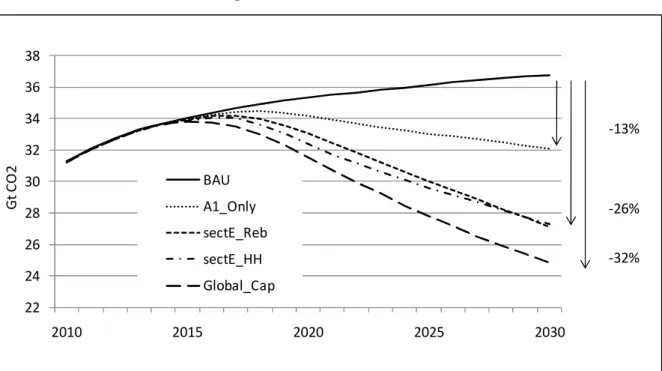
The global emission trajectory11 is the highest in the BAU scenario and the lowest in Global_Cap (Figure 1). In the A1_Only scenario, the emission trajectory is closer to BAU than to Global_Cap, for two reasons. First, a cap on the emissions of Annex I countries can only hope to attenuate 50% of the cumulated emission over 2013-2030, since in our BAU scenario these countries emit 50% of the cumulated emissions over 2013-2030. Second, as is apparent in Figure 3 below, a small part of the abatement in developed countries "leaks" to developing countries,. This carbon leakage12 is very limited (the leakage-to-reduction ratio is only 8% in 2030) and comes mainly through two mechanisms: first, the world prices of oil, coal and natural gas are reduced by CO2 abatement measures in developed countries (cf. Figure 11-13 in Appendix 2), thereby increasing fossil fuels consumption and hence
emissions, in developing countries; second, the climate policy increases the production cost of developed countries’ producers compared to those in developing countries, thereby reducing the competitiveness of energy-intensive industries of developed countries. As a consequence, developing countries export more, and import less, energy-intensive goods, contributing further to increasing their emissions.
10 Admittedly, in the sectoral crediting mechanism proposed by the European Commission (2009) and in most
other proposals, the crediting target would be set at a higher level than expected emissions with a CO2 price.
Developing countries would then benefit from a transfer of CO2 allowances from developed countries. Such
transfers were not included in order to disentangle the impact of transfers from the other economic mechanisms.
11
The emissions considered here are energy-related CO2 emissions.
12 Carbon leakage is defined as the increase in emissions in the rest of the world, following a climate policy in a
Figure 1. Global CO2 emissions 22 24 26 28 30 32 34 36 38 2010 2015 2020 2025 2030 G t C O 2 BAU A1_Only sectE_Reb sectE_HH Global_Cap -26% -32% -13%
The most interesting point in Figure 1 is that emissions in the two sectoral scenarios are much closer to Global_Cap than to A1_Only. In 2030, global abatement compared to the BAU scenario reaches 32% in Global_Cap, 26% under the two sectoral scenarios and only 13% under A1_Only, i.e. in 2030, both sectoral scenarios reach 80% of the abatement (compared to BAU) of Global_Cap.13 Two factors explain this positive result: the potential for emissions reduction in the power generation sector of non-Annex I countries’ is both important and relatively easy to reach. Electricity generation is the main emitting sector in the BAU scenario, contributing 41% of non-Annex I countries’ emissions in 2030. Moreover, these emissions are relatively easy to abate given that there are low carbon power generation technologies and they become profitable at moderate levels of carbon pricing. In this regard, the results are in line with existing studies that reveal large reduction potentials in the power sector, accessible at low carbon prices (see for instance Clapp et al., 2009).
Figures 2 and 3 detail the CO2 emissions from Annex I countries and non-Annex I countries respectively. Unsurprisingly, Annex I emissions follow the same trajectory in all policy scenarios, below BAU emissions trend. Indeed, the AI_only, SectE_HH and SectE_Reb scenarios correspond to architectures in which Annex I countries are allocated the same emissions as in Global_Cap, without quota transfers between Annex I and non-Annex I.
13
Alternative scenarios could be assessed, in particular those in which the targets for Annex I countries would be changed, thereby making up for any extra emissions in non-Annex I countries , though the overall target remains unchanged (See Bosetti and Victor (2010). However, bringing global emissions down to 25 Gt CO2 in 2030
without climate policy in developing countries (as in our Global_Cap scenario) would require an extremely high and completely unrealistic CO2 price in Annex I countries. Thus, with the exception of the BAU scenario, the
Figure 3 shows that the emissions of non-Annex I countries are above BAU level in AI_only, due to the leakage mechanisms explained above. The emissions of non-Annex I countries are the lowest in the scenario in which all sectors of their economies are subject to carbon pricing (Global_Cap) though they lie between Global_Cap and BAU levels in both sectoral scenarios. Further examination of this point requires separate analysis of the emissions trends of the power generation sector (Figure 4) and the energy intensive industry (Figure 5).
Figure 2. Annex I CO2 emissions
0 2 4 6 8 10 12 14 16 18 20 2010 2015 2020 2025 2030 G t C O 2 BAU
All other scenarios
Figure 3. Non-Annex I CO2 emissions
0 2 4 6 8 10 12 14 16 18 20 2010 2015 2020 2025 2030 G t C O 2 A1_Only BAU sectE_Reb sectE_HH Global_Cap
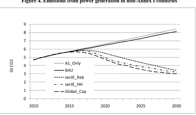
Figure 4 focuses on emissions from electricity generation in non-Annex I countries. Emissions are close to Global_Cap, only a little higher, in both sectoral scenarios,. In Global_Cap, electricity consumption is reduced since the climate policy affects overall economic activity (Cf. Figure 6 below). Emissions are slightly higher in SectE_Reb than in SectE_HH. Indeed, in the former scenario, the rebate partially offsets the price increase, hence electricity generation is less impacted and the decrease in emissions is lower.
Figure 4. Emissions from power generation in non-Annex I countries
0 1 2 3 4 5 6 7 8 9 2010 2015 2020 2025 2030 G t C O 2 A1_Only BAU sectE_Reb sectE_HH Global_Cap
In SectE_HH and, to a much lesser extent, in SectE_Reb, emissions from the energy-intensive industry in developing countries increase compared to BAU (cf. Figure 5). This inter-sectoral emission leakage - from power generation to industry - has two different sources or
mechanisms:
(i) the rise in electricity price (Cf. Section 3.3 below) induces industry to substitute fossil fuels for electricity, and
(ii)the competitiveness gains of non-Annex I industries, with respect to those Annex countries’ industries that are subject to carbon pricing, increase the volume of industrial production.
Industrial production is also increased in some cases, as we will see in Figure 6, by more domestic demand for industrial goods in non-Annex I countries, driven by higher overall economic activity. The first of these two mechanisms is dominant in the SectE_HH scenario. For instance, coal intermediate consumption, per unit of industrial good produced, is 10% higher in China, in 2030, in the SectE_HH scenario compared to the BAU level. In this
scenario, industrial production remains below its BAU level until 2026 and is 1.8% above in 2030.
By contrast, in the SectE_Reb scenario, the rise in electricity price plays only a marginal role and is limited to the first years of the period considered: the electricity prices (Cf. Section 3.3) become lower than in the BAU scenario after 2020. For example, coal intermediate
consumption, per unit of industrial good produced in China, is only 1% higher in the SectE_Reb scenario compared to that of the BAU level in 2020. After 2020, the inverse mechanism is operative: lower electricity prices drives substitution away from fossil fuels in the industry sector. For example, coal intermediate consumption per unit of industrial good produced in China is 0.4% lower in 2030. However, this is counterbalanced by a larger volume of industrial production, i.e. the second source of underlying sectoral leakage mentioned above. The results show, for instance, that in this SectE_Reb scenario Chinese industrial production is, by 2018, larger than in BAU scenario and is approximately 2.5% above its BAU level from 2025-2030.
Despite the fact that the two mechanisms can have different respective contributions and sometimes work against each other, the combination of the two always has the same net result: an increase in overall emissions from energy-intensive industry in both SectE_HH and SectE_Reb scenarios compared to the BAU level. The increase is more pronounced in the SectE_HH scenario, which explains why, in 2030, though aggregate non-Annex I emissions are a little lower in SectE_Reb than in SectE_HH (Figure 3), non-Annex I emissions from power generation remain higher in SectE_Reb than in SectE_HH.
As shown in Figure 5, emissions from the energy-intensive industry in non-Annex I countries, in the A1_Only scenario, are a little higher than in BAU, because developing countries’ CO2 -intensive industries production is larger. Indeed, since these industries are not subject to carbon pricing while Annex I countries’ industries are, developing countries export more of these goods to, and import less from, developed countries. A small amount of carbon leakage is thus thereby generated.
Figure 5. Emissions from the energy-intensive industry in non-Annex I countries 0 1 2 3 4 5 6 2010 2015 2020 2025 2030 G t C O 2 sectE_HH sectE_Reb A1_Only BAU Global_Cap
3.2. GDP losses: The sectoral approach with rebates entails much
lower GDP losses in developing countries
In Figure 6, in the Global_Cap scenario, the transitory GDP losses following the introduction of carbon pricing in developing countries are significant: they reach more than 3% (compared to BAU) around 2018. These important short-term macroeconomic losses are due to the conjunction of installed productive capital inertia, imperfect anticipations, and rigidities in labour markets14 that prevents the rapid adaptation of the economy to the shock on prices induced by the carbon tax. After 2018, GDP progressively catches up with its BAU level. This partial catch-up is due to induced technological change mechanisms (Crassous et al., 2006) and less vulnerability to peak oil. The economies’ vulnerability to peak oil in baseline scenarios is due to the imperfect expectation of oil price increase when producers are
constrained by the depletion of resources. This imperfect expectation is partially corrected by carbon pricing: technical change, and consumption structure change induced by climate policies, reduce economies’ dependence on oil. Nevertheless, the prospect of such short-term losses would be difficult to accept for the governments of developing countries.
Comparing Figures 6 and 8 reveals that the costs of a global cap-and-trade system, such as Global_Cap scenario, are significantly higher for non-Annex I, than for Annex I, countries: the peak GDP losses reach 3% of the reference GDP vs. 0.6%.15 This explains why such
14
Guivarch et al. (2010) analyze in detail the influence of labour markets rigidities on the costs of climate policies.
15Note, however, that the significant difference in the order of magnitude of non-Annex I and Annex I costs is
moderated if results are presented in terms of delays in reaching the GDP level of the BAU scenario. Indeed, the peak GDP loss corresponds to a 10 month growth delay for non-Annex I countries, while it represents a 5 month delay for Annex I countries.Presented that way, the costs for non-Annex I countries still appear higher than for
architecture is unacceptable for non-Annex I countries. To make a global cap-and-trade system more attractive to non-Annex I countries, quota allocation rules that are more favourable to these countries might be considered. However, these would entail very
significant transfers from Annex I to non-Annex I countries. For example, if we calculate ex post16 the additional transfers necessary to cancel non-Annex I GDP losses in our Global_Cap scenario, they peak at 1.2% of Annex I GDP in 2018 and are above 1% over the 2017-2027 period. Such large transfers engender the “revenue management” issues raised in Section 1.17 It also raises the question of acceptability for Annex I countries and the subsequent credibility concern, if one remembers that Annex I countries never enforced the objective of contributing 0.7% of their GDP to overseas aid.
In SectE_HH, the losses are lower but still reach 2% around 2018. Note that in this scenario, GDP is actually higher than in BAU after 2029, mainly because developing countries benefit from lower world energy prices. In SectE_Reb, GDP losses are always less than 1% and GDP is higher than BAU as soon as 2020.
From Figures 3 and 6, it can be seen that in the late 2020s, SectE_Reb provides a similar emissions reduction than SectE_HH though for a much lower impact on GDP in developing countries. This result may be a surprise since in a simple model without pre-existing
distortion, and without leakage, using the auction or tax revenues as a production subsidy increases the abatement cost for a given abatement target compared to a lump-sum
distribution of the revenues (e.g. Fischer, 2001). The explanation of this surprising result is that in our setting, a lump-sum distribution of the revenues exacerbates the pre-existing distortions, and generates inter-sectoral emissions leakage (from electricity generation to industry), more than a distribution of the revenues as a decrease in pre-existing production taxes or as a production subsidy.
Finally, in the A1_Only scenario, developing countries’ GDP increases, compared to BAU for two reasons: first, their production of CO2-intensive goods increases due to competitiveness gains vis-à-vis Annex I regions (as explained above) and they benefit from lower world energy prices. Indeed, lower energy prices have a positive effect on households’ real income (The Slutsky effect, Slutsky, 1915), and lead to more consumption, hence production.
those of Annex I, but the relative sizes of the costs are less stark. This is linked to the fact that developing countries grow faster than developed countries.
16We make the daring assumption that the transfers would be macroeconomically neutral. McKibbin et al.
(1999), among others, have demonstrated that large transfers do have macroeconomic implications. The simple ex post calculation given here therefore has an indicative value only.
17 The financial inflows linked to the selling amount of emission quotas to up to several percents of the
countries’ GDP in the Global_Cap scenario (e.g. 3% for Africa in 2029 and 2.5% for India in 2027). For comparison, the financial flows from oil and gas represented 1.5% of the Dutch GDP at the end of the 1960s (OECD,National Accounts of OECD countries 1961-1978, Detailed Tables, Volume II). Such orders of magnitude tend to confirm the risk of “Dutch disease” symptoms linked to quota exchanges.
GDP losses in China18 follow the same trends, but with higher magnitudes (Figure 7), due to its high CO2-intensity: 0.6 kg CO2/US$ PPP in 2007 vs. 0.47 for the world average and 0.48 for non-Annex I countries in average (IEA, 2009a).
Figure 6. GDP losses in non-Annex I countries
-4,0% -3,5% -3,0% -2,5% -2,0% -1,5% -1,0% -0,5% 0,0% 0,5% 1,0% 1,5% 2010 2015 2020 2025 2030 R e a l G D P v a ri a ti o n s (% B A U ) A1_Only sectE_Reb sectE_HH Global_Cap
Figure 7. China GDP losses
-7,0% -6,0% -5,0% -4,0% -3,0% -2,0% -1,0% 0,0% 1,0% 2,0% 3,0% 2010 2015 2020 2025 2030 R e a l G D P v a ri a ti o n s (% B A U ) A1_Only sectE_Reb sectE_HH Global_Cap
18 The case of China is singled out because it is the first CO
2 emitter. Moreover, the Copenhagen conference
The picture differs for Annex I countries whose GDP is always lower than in BAU (Cf. Figure 8). The loss is the lowest in Global_Cap because in the other scenarios, the
competitiveness of Annex I industries is affected because they are subject to carbon pricing whilst the industries of non-Annex I countries are not. Moreover, world energy prices are the lowest under Global_Cap (See Appendix 2). The highest losses occur in the A1_Only and SectE_Reb scenarios, with very close values, whereas losses are intermediate for SectE_HH. What explains this last result is that in SectE_HH, the competitiveness of the industries of developed countries is less affected because developing countries producers’ suffer from a higher electricity price than in A1_Only and SectE_Reb.
Figure 8. GDP losses in Annex I countries
-1,2% -1,0% -0,8% -0,6% -0,4% -0,2% 0,0% 0,2% 2010 2015 2020 2025 2030 R e a l G D P V a ri a ti o n s (% B A U ) Global_Cap sectE_HH sectE_Reb A1_Only
3.3. Impacts on electricity markets are much milder with rebates
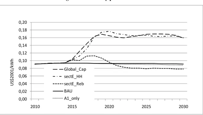
As shown in Figure 9, under Global_Cap and SectE_HH, the electricity price19 almost doubles in China, both compared to BAU and to the historical level. The main reason for this increase is that electricity producers pass on the cost of allowances to consumers. A second reason is that more expensive production technologies partly replace the relatively cheap fossil fuel technologies.In SectE_Reb, the electricity price increases much less: the price increase due to the CO2 allowances is partially offset by the subsidy. More surprising is the fact that after 2020 electricity price actually drops below the BAU level. There are two explanations for this. First, some learning-by-doing occurs in low carbon technologies, which are used more in the
19
The electricity price shown here is the production price, i.e. including production taxes and subsidies (if any), averaged over time slices. It is not the final consumption price, which differs across sectors and includes consumption taxes and subsidies.
scenarios with climate policies. Second, in Imaclim-R, electricity producers set their price according to the complete cost of electricity generation over the life time of their power plants, using the current fossil fuel prices as the expectation of the future prices. However, in the BAU scenario considered, gas and oil prices increase (Cf. Figure 11 and 12 in Appendix 2). Thus the electricity generation mix in BAU is too carbon-intensive compared to the ex post private optimum.20 A CO2 price helps to correct this myopia by pushing producers to reduce the share of fossil fuel in their generation mix.
Electricity production (Figure 10) mirrors electricity price. In Global_Cap and SectE_HH, electricity generation is roughly stabilised in China, whereas its growth follows the BAU level in the A1_Only and SectE_Reb scenarios.
As Table 1 and Table 2 show, the same trends occur in other regions except Brazil, which benefits from a large share of hydropower and is thus less affected by carbon pricing. The same mechanisms as in the Chinese case, described above, are valid for other regions. They lead to a significant increase in the electricity prices compared to the BAU level in 2020. This phenomenon is particularly pronounced in both Global_Cap and SectE_HH scenarios and continues until the end of the period. In the SectE_Reb scenario the electricity price increase is moderate in 2020 and a price decrease is observed in 2030.
Figure 9. Electricity prices in China
0,00 0,02 0,04 0,06 0,08 0,10 0,12 0,14 0,16 0,18 0,20 2010 2015 2020 2025 2030 U S$ 2 0 0 1 /k W h Global_Cap sectE_HH sectE_Reb BAU A1_only
Figure 10. Electricity production in China 3000 3500 4000 4500 5000 5500 6000 6500 2010 2015 2020 2025 2030 T W h A1_Only sectE_Reb BAU Global_Cap sectE_HH
Table 1. Electricity price variation (% BAU) in 2020
Global_cap secE_HH secE_Reb A1_only
China 77% 90% 3% -1%
India 61% 66% 4% -1%
Rest of Asia 55% 65% 6% -2%
Africa 67% 74% 7% -2%
Brazil 6% 8% 3% 1%
Table 2. Electricity price variation (% BAU) in 2030
Global_cap secE_HH secE_Reb A1_only
China 74% 75% -14% -3% India 39% 46% -8% -3% Rest of Asia 48% 46% -8% -4% Africa 58% 57% -4% -3% Brazil 3% 2% 3% 0%
Conclusion
Many experts and stakeholders have proposed sectoral targets for developing countries. This article provides the first macroeconomic assessment of such proposals using a global multi-region, multi-sector general equilibrium model. More precisely, scenarios are assessed in which both (i) developed countries apply Kyoto-type targets and (ii), emissions in developing countries from power generation are subject to the same CO2 price as those in developed countries. These scenarios are compared to a global cap-and-trade architecture, in terms of
both the macroeconomic cost for emerging and developing countries and in terms of emission reductions achieved.
The results indicate that a sectoral target for developing countries, limited to the electricity sector, is able to provide around 80% of the global energy-related CO2 emission reductions achieved in a global cap-and-trade system. Moreover, if this sectoral target is implemented as an emission trading system, or as an emissions tax with revenues distributed to electricity generation firms in the form of a decrease in pre-existing production taxes, or a production subsidy, the economic impact in developing countries is milder than that of a global cap-and-trade system: GDP losses are much lower and so is the impact on the electricity price. Such sectoral approaches may thus appear more acceptable for non-Annex I countries than a global cap-and-trade scheme. Equally, they lead to significant emissions reduction. They thus constitute an interesting option to combine “common but differentiated responsibilities” with “meaningful participation” in the design of post-Kyoto architectures (all the more as the Copenhagen Accord leaves the door open to these new sectoral approaches).
The scenarios assessed are intentionally, however, very stylized. In the real world, if a sectoral approach is applied, it will certainly feature a higher level of differentiation across regions including, inter alia, a staged implementation with entry dates depending on development levels, price differentiation and international transfers. Moreover, there are numerous barriers to the rational use of electricity, which are unlikely to be removed by carbon pricing policy alone. Therefore, supplementary measures to foster a real improvement in the energy efficiency of electricity end-uses will be needed to make sectoral policies that target power generation effective (IEA, 2009c). Furthermore, the analysis presented here does not take into account the fact that in many developing countries, electricity markets are not liberalized and regulated tariffs often include important subsidies to electricity consumption. This is one important limitation of the study,21 and forms one of the main difficulties for the implementation of a sectoral policy for power generation.
In the longer term, the share of emissions from other sectors, especially transportation, will grow, as they did in developed countries, in developing countries. Moreover, with economic growth, the major emitters in the developing world will have a better capacity to make commitments and seek to control all emitting sectors. Consequently, the sectoral approach presented here should be seen as a transitory policy, rather than as an alternative to a more global and general approach.
21
In a case study using a version of Imaclim-R that includes regulated tariffs and subsidies to electricity consumption, Mathy and Guivarch (2010) try to go beyond this limitation and analyze the suboptimalities in the Indian power sector and their implications for climate policies,.
Appendix 1. The Imaclim-R model
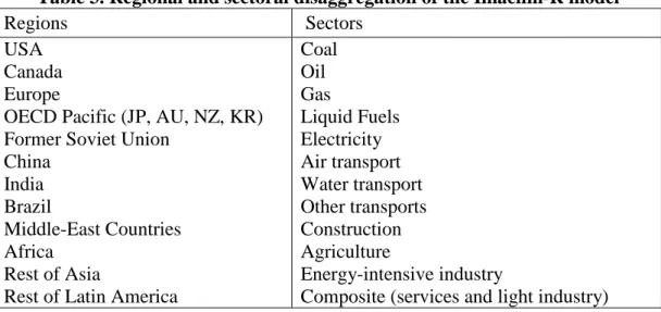
Imaclim-R is a hybrid recursive general equilibrium model of the world economy, divided into 12 regions and 12 sectors (Table ) and solved in a yearly time step (Sassi et al., 2010). The base year of the model (2001) is built on the GTAP-6 database, which provides a balanced Social Accounting Matrix (SAM) of the world economy. The original GTAP-6 dataset has been modified to (i) aggregate regions and sectors according to the Imaclim-R mapping, and (ii) accommodate the 2001 IEA energy balances, in an effort to base Imaclim-R on a set of hybrid energy-economy matrixes.
Note that the emission trajectory22 simulated in the business-as-usual scenario considered in the article is very close to the IEA CO2 emissions data (IEA, 2009a) over the 2002-2007 period: according to the IEA, CO2 world emissions from fossil fuel combustion grew from 23.7 Gt CO2 in 2001 to 29.0 in 2007, whereas the output of the Imaclim-R model is 29.1 Gt CO2 for 2007.
Table 3. Regional and sectoral disaggregation of the Imaclim-R model
Regions Sectors
USA Canada Europe
OECD Pacific (JP, AU, NZ, KR) Former Soviet Union
China India Brazil Middle-East Countries Africa Rest of Asia
Rest of Latin America
Coal Oil Gas Liquid Fuels Electricity Air transport Water transport Other transports Construction Agriculture Energy-intensive industry
Composite (services and light industry)
As a general equilibrium model, Imaclim-R provides a consistent macroeconomic framework to assess the energy-economy relationship. Specific efforts have been devoted to building a modelling architecture allowing the incorporation of technological information coming from bottom-up models and experts’ judgement within the simulated economic trajectories. The rigorous incorporation of information about how final demand and technical systems are transformed by economic incentives is allowed for by the existence of physical variables that explicitly characterise equipments and technologies (e.g. the efficiency of cars, the intensity of production in transport etc.). The economy is then described in both money-metric terms and physical quantities, the two dimensions being linked by a price vector. This dual vision of the economy is a precondition to guarantee that the projected economy is supported by a realistic technical background and, conversely, that any projected technical system corresponds to realistic economic flows and consistent sets of relative prices.
22 In the current version of the model, the emissions covered are energy-related CO
The full potential of this dual representation could not be exploited without abandoning the use of conventional aggregate production functions that, after Berndt and Wood (1975) and Jorgenson (1981) were admitted to mimic the set of available techniques: it is arguably almost impossible to find mathematical functions flexible enough to cover large departures from the reference equilibrium and to encompass different scenarios of structural changes resulting from the interplay between consumption styles, technologies and localisation patterns (Hourcade 1993). In Imaclim-R the absence of formal production functions is compensated by a recursive structure that organizes a systematic exchange of information between:
• An annual static equilibrium module with Leontief production functions (fixed equipment stocks and intensities of intermediary inputs, especially labour and energy; but a flexible utilisation rate). Solving this equilibrium at some year t provides a snapshot of the economy: information about relative prices, output levels, physical flows etc.
• Dynamic modules, including demography, capital dynamics and sector-specific reduced forms of technology-rich models, most of which assess the reactions of technical systems to the previous static equilibriums. These reactions are then sent back to the static module in the form of updated input-output coefficients to calculate year (t+1) equilibrium.
Between two equilibriums, technical choices are fully flexible for new capital only; the input-output coefficients and labour productivity are modified at the margin because of fixed techniques embodied in existing equipment and resulting from past technical choices. This general putty-clay assumption is critical to represent the inertia of technical systems and the perverse effect of economic signals volatility.
Imaclim-R thus generates economic trajectories by solving successive yearly static equilibriums of the economy interlinked by dynamic modules. Within the static equilibrium, in each region the demand for each good derives from household consumption, government consumption, investment and intermediate uses from the production sectors. This demand can be provided either by domestic production, or imports, and all goods and services are traded on world markets. Domestic and international markets for all goods – excluding labour – are cleared by a unique set of relative prices that depend on the demand and supply behaviours of representative agents. The calculation of this equilibrium determines relative prices, wages, labour, quantities of goods and services, and value flows.
The dynamic modules shape the accumulation of capital and its technical content; they are driven by economic signals (such as prices or sectoral profitability) that emerge from former static equilibriums. They include the modelling of (i) the evolution of capital and energy equipment stock, described in both vintage and physical units (such as number of cars, housing square meter, transportation infrastructure), (ii) technological choices of economic agents described as discrete choices in explicit technology portfolios for key sectors such as electricity, transportation and alternative liquid fuels, or captured through reduced form of
technology rich bottom up models, and (iii) endogenous technical change for energy technologies (with learning curves).
In this framework, the main exogenous drivers of economic growth are population and labour productivity dynamics. However, international trade, particularly that of energy commodities, and imperfect markets for both labour (wage curve) and capital (constrained capital flows, varying utilisation rates of productive capacities), significantly impact on economic growth.
Appendix 2. Impact on world energy and CO
2prices
The world prices of oil, natural gas and coal are endogenous and result from demand
dynamic, availability of substitutes and depletion of resources (Cf. Waisman et al., 2010, for a presentation of this part of the model).
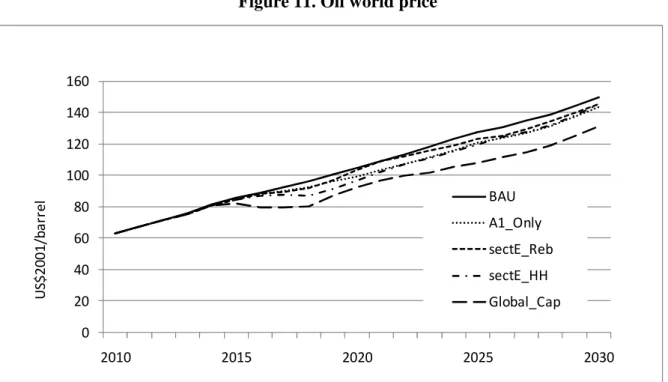
As shown in Figure 11, the world energy prices are the highest in BAU and the lowest in Global_Cap. More generally, the higher the emissions, the higher the energy prices, because the implicit supply curve of fossil fuels is upward-slopping.
Figure 11. Oil world price
0 20 40 60 80 100 120 140 160 2010 2015 2020 2025 2030 U S$ 2 0 0 1 /b a rr e l BAU A1_Only sectE_Reb sectE_HH Global_Cap
Figure 12. Gas world price 0 100 200 300 400 500 600 700 2010 2015 2020 2025 2030 U S$ 2 0 0 1 /T E P BAU A1_Only sectE_Reb sectE_HH Global_Cap
Figure 13. Coal world price
0 20 40 60 80 100 120 2010 2015 2020 2025 2030 U S$ 2 0 0 1 /T E P BAU A1_Only sectE_Reb sectE_HH Global_Cap
As we can see in Figure 14, the CO2 price is almost equal across all scenarios but a little higher in Global_Cap. The explanation is that in this scenario, the fossil fuel prices are lower, so a higher CO2 price is required to reach a given emissions level in Annex I countries.
Figure 14. CO2 price 0 20 40 60 80 100 120 2010 2015 2020 2025 2030 U S$ 2 0 0 1 /t C O 2 Global_cap Annex_I_only Elec_Rebates Elec_Households
References
Amatayakul, W., Berndes G., Fenhann J., 2008. Electricity sector no-lose targets in
developing countries for post-2012: Assessment of emissions reduction and reduction credits,
CD4CDM Working Paper No.6, December, UNEP Risoe centre, Roskilde, Denmark [available at www.indiaenvironmentportal.org.in/files/ElectricityTargetsDCpost2010.pdf]. Amatayakul, W., and J. Fenhann, 2009. Electricity sector crediting mechanism based on a
power plant emission standard: a clear signal to power generation companies and utilities planning new power plants in developing countries post-2012, CD4CDM Working Paper
No.7, July, UNEP Risoe centre, Roskilde, Denmark [available at
www.indiaenvironmentportal.org.in/files/ElectricityCreditingPlantsEmissionStandard.pdf]. Berndt, E.R., and D.O. Wood, 1975. Technology, prices, and the derived demand for energy.
The Review of Economics and Statistics, LVII(3), August
Bosetti, V. and Victor, D.G. 2010. Politics and Economics of Second-Best Regulation of
Greenhouse Gases: The Importance of Regulatory Credibility. FEEM Working Paper No.
29.2010 [available at ssrn.com/abstract=1593586].
CISDL (Centre for International Sustainable Development Law), 2002. The Principle of
Common But Differentiated Responsibilities: Origins and Scope. [available at
www.cisdl.org/pdf/brief_common.pdf]
Clapp, C., K. Karousakis, B. Buchner and J. Chateau, 2009. National and sectoral GHG mitigation potential: A comparison across models, OECD, 16 November
Crassous, R., Hourcade, J.-C., Sassi, O., 2006. Endogenous structural change and climate targets : modeling experiments with Imaclim-R, Energy Journal, Special Issue on the Innovation Modeling Comparison Project
Ellerman, A.D., 2008. New Entrant and Closure Provisions: How do they distort? Energy Journal, 29, Special Issue
European Commission, 2009. Commission staff working document accompanying the
Communication from the Commission to the European Parliament, the Council, the European Economic and social Committee and the Committee of the Regions, Stepping up international climate finance: A European blueprint for the Copenhagen deal {COM(2009) 475}. Brussels,
SEC(2009) 1172/2, September
Fischer, C., 2001. Rebating Environmental Policy Revenues: Output-Based Allocations and
Tradable Performance Standards. RFF Discussion Paper 01-22
G77 and China, 2008. Submission of the G77 and China. Contact Group on Shared Vision. December 2008. [available at
http://unfccc.int/files/kyoto_protocol/application/pdf/philippinesctgsharedvision061208.pdf]. Godard, O., 2009. Quelle architecture internationale pour la politique climatique ? 1. Les
www.enseignement.polytechnique.fr/economie/chaire-business-economics/OG-Architectureclimat-181009REV2110.pdf].
Guivarch, C., Crassous, R., Sassi, O. and Hallegatte, S. 2010. The costs of climate policies in
a second best world with labour market imperfections. Climate Policy (forthcoming)
Guivarch C., Hallegatte S., Crassous R., 2009. The Resilience of the Indian Economy to Rising Oil prices as a validation test for a Global Energy-Environment-Economy CGE model, 2009, Energy Policy 37, November
Hahn, R., 1984. Market power and transferable property rights. Quarterly Journal of
Economics, 99: 735–765.
Hourcade, J.C., 1993. Modeling long-run scenarios – methodology lessons from a prospective study on a low-CO2 intensive country, Energy Policy 21(3): 309-326
IEA, 2009a. CO2 emissions from fossil fuel combustion - Highlights, International Energy Agency, Paris
IEA, 2009b. World Energy Outlook, International Energy Agency, Paris
IEA, 2009c. Sectoral Approaches in Electricity – Building Bridges to a Safe Climate, International Energy Agency, 186 pages, ISBN 978-92-64-06872-8
IPCC, 2000. Special Report on Emissions Scenarios : a special report of Working Group III of the Intergovernmental Panel on Climate Change. Cambridge University Press, New York, NY (US).
Jorgenson, DW, 1981. Energy prices and productivity growth, Scandinavian Journal of
Economics, 83(2): 164-179
Mathy, S., Guivarch, C. 2010. Climate policies in a second-best world - A case study on India. Energy Policy 38(3): 1519-1528.
McKibbin, W., M. Ross, R. Shackleton, P. Wilcoxen, 1999. Emissions Trading, Capital Flows and the Kyoto Protocol. Energy Journal. Volume 20, Special Issue
Meckling, J. O. and Chung, G. Y., 2009. Sectoral approaches for a post-2012 climate regime: a taxonomy. Climate Policy, 9(6): 652-668
Meunier, G. and J.-P. Ponssard, 2009. A proposal combining sectoral approaches in
developing countries with cap and trade in industrialized countries. Working paper, Ecole
Polytechnique [available at www.enseignement.polytechnique.fr/economie/chaire-business-economics/meunierponssardsectoralapproaches.pdf].
Philibert, C., 2000. How could emissions trading benefit developing countries, Energy Policy, 28 (13), p.947-956, Nov.
Quirion, P., 2009. Historic versus output-based allocation of GHG tradable allowances: a comparison. Climate Policy, 9: 575–592
Sassi O., Crassous R., Hourcade J.-C., Gitz V., Waisman H., Guivarch C., 2010. ‘Imaclim-R : a modelling framework to simulate sustainable development pathways’, International Journal
of Global Environmental Issues Vol 10, n°1, p 5-24.
Sawa, Akihiro. 2008. A Sectoral Approach as an Option for a Post-Kyoto Framework. Discussion Paper 08-23, Harvard Project on International Climate Agreements, Belfer Center for Science and International Affairs, Harvard Kennedy School.
Schmidt, J., Helme, N., Lee, J., and Houdashelt, M., 2008. Sector-Based Approach to the Post-2012 Climate Change Policy Architecture, Climate Policy 8, Earsthscan, London, pp. 494-515.
Slutsky, E.E. 1915. On the Theory of the Budget of the Consumer. Giornale degli Economisti Vol 51, n°1, p 1-26.
Strand, J., 2009. "Revenue management" effects related to financial flows generated by
climate policy. Background paper to the 2010 World Development Report, Policy research
working paper 5053, World Bank
Tirole, J., 2009. Politique climatique : une nouvelle architecture internationale, Rapport du Conseil d'analyse économique, La Documentation française, Paris, octobre
UNFCCC, 2009. Copenhagen Accord, 18 December [available at unfccc.int/resource/docs/2009/cop15/eng/l07.pdf].
Waisman H., Sassi O., Rozenberg J., Hourcade J.-C., 2010. Drivers and macroeconomics of
the Peak Oil, CIRED Working Paper
Weitzman, M., 1974. "Prices vs. Quantities", Review of Economic Studies, 41(4): 447-91 WRI, 2009a. Summary of UNFCCC Submissions, September 18 [available at
pdf.wri.org/working_papers/unfccc_submissions_summary_2009-09-18.pdf]. WRI, 2009b. Climate Analysis Indicators Tool (CAIT) 7.0 database, [available at cait.wri.org/].