Acoustic scattering by axisymmertic finite-length bodies with application to fish : measurement and modeling

Acoustic Scattering by Axisymmetric Finite-length Bodies with

Application to Fish: Measurement and Modeling

by

D. Benjamin Reeder B.S., Clemson University (1988)

Submitted to the Department of Ocean Engineering, MIT and the Department of Applied Ocean Physics and Engineering, WHOI

in partial fulfillment of the requirements for the degree of Doctor of Philosophy

at the

MASSACHUSETTS INSTITUTE OF TECHNOLOGY AND THE

WOODS HOLE OCEANOGRAPHIC INSTITUTION June 2002

@

BARKER

MASSACHUSETITS INSTITUTE

OF TECKNOLOGY

AUG 2 1 2002

LIBRARIES

The author hereby grants to Massachusetts Institute of Technology and the

Woods Hole Oceanographic Institution permission to reproduce and to distribute copies of this thesis document in whole or in part.

Signature of Author.... ... ...

Department of Ocean Engineering, MIT and the Department of Applied Ocean Physics and Engineering, WHOI n May 1, 2002 Certified by ...

Certified by ...

Dr. Timothy K. Stanton Senior Scientist, WHOI Thesis Advisor

Prof. Arthur B. Baggeroer Professor, MIT Academic Advisor

A ccepted by ... I. ...

Acoustic Scattering by Axisymmetric Finite-length Bodies with Application to Fish: Measurement and Modeling

by

D. Benjamin Reeder

Submitted to the Department of Ocean Engineering, MIT and the Department of Applied Ocean Physics and Engineering, WHOI

on May 1, 2002, in partial fulfillment of the requirements for the degree of

Doctor of Philosophy

Abstract

This thesis investigates the complexities of acoustic scattering by finite bodies in general and

by fish in particular through the development of an advanced acoustic scattering model and

detailed laboratory acoustic measurements. A general acoustic scattering model is developed that is accurate and numerically efficient for a wide range of frequencies, angles of orientation, irregular axisymmetric shapes and boundary conditions. The model presented is an extension of a two-dimensional conformal mapping approach to scattering by irregular, finite-length bodies of revolution. An extensive series of broadband acoustic backscattering measurements has been conducted involving alewife fish (Alosa pseudoharengus), which are morphologically similar to the Atlantic herring (Clupea harengus). A greater-than-octave bandwidth (40-95 kHz), shaped, linearly swept, frequency modulated signal was used to insonify live, adult alewife that were tethered while being rotated in 1-degree increments over all angles of orientation in two planes of rotation (lateral and dorsal/ventral). Spectral analysis correlates frequency dependencies to morphology and orientation. Pulse compression processing temporally resolves multiple returns from each individual which show good correlation with size and orientation, and demonstrate that there exists more than one significant scattering feature in the animal. Imaging technologies used to exactly measure the morphology of the scattering features of fish include very high-resolution Phase Contrast X-rays (PCX) and Computerized Tomography (CT) scans, which are used for morphological evaluation and incorporation into the scattering model. Studies such as this one, which combine scattering models with high-resolution morphological information and high-quality laboratory data, are crucial to the quantitative use of acoustics in the ocean.

Thesis Advisor: Dr. Timothy K. Stanton Title: Senior Scientist, WHOI

Academic Advisor: Prof. Arthur B. Baggeroer Title: Professor, MIT

Acknowledgments

Science, as in life, is not conducted in a vacuum: this thesis is the result of contributions by many individuals, both directly and indirectly. Although it is impossible to recognize everyone who has had an impact on this research, I would like to recognize a few key individuals.

I am deeply grateful to the U.S. Navy, the Oceanographer of the Navy and the Office of Navy Research whose generous support made my participation in the Joint Program possible. I genuinely appreciate the guidance and support given to me by my thesis advisor, Dr. Tim Stanton, whose enthusiasm and energy for science is contagious. He was always available for discussion and questions, no matter how busy he was as Chair of the AOPE department at WHOI. I would also like to thank Prof. Arthur Baggeroer, for his advice and direction as my academic advisor at MIT, and for our many conversations about the Navy. Thanks also to the other members of my Thesis and Defense Committees: Dr. Ken Foote, Dr. Peter Wiebe and Dr. Jim Lynch, whose advice and comments regarding my research were greatly appreciated. I am indebted to Dr. Dezhang Chu for his many answers to my many questions regarding scattering theory, modeling and computing over the last five years. I would also like to thank Dr. Mike Jech for his involvement in the experimental portion of this research; Dr. Daniel T. DiPerna who proposed the scattering theory in Chapter 2 and provided much guidance during the course of this work; Dr. Trevor Francis of the University of Birmingham, UK, for generously providing the BEM calculation for Fig. 2-8; Falmouth Hospital for performing the CT scans of the alewife; Falmouth Animal Hospital for the use of their x-ray machine; Benthos, Inc. for the use of their test tank for the acoustic measurement portion of the study; Dr. Andrew Stevenson, Dr. D. Gao and Dr. Steve Wilkins at Australia's Commonwealth Scientific and Industrial Research Organisation (CSIRO), who have been very generous in their PCX imaging of the fish; and Dr. Hanu Singh, Dr. Andone Lavery and the Graphics Department at the Woods Hole Oceanographic Institution for help with image processing.

Words are inadequate to express my wholehearted thanks to my wife, Lisa, and my daughter, Emma, for their love, patience and support for me during the last five years. Their dedication and commitment to the success of this project were as crucial as my own. I would also like to thank my father, Max, for teaching me to value hard work and my mother, Jeanette, who inspired me to pursue science and engineering as a profession. Finally, I would like to thank God, who has given me this wonderful opportunity to study the physics of acoustic scattering, and without whom life and science would be meaningless.

Contents

1 Introduction 7

1.1 Historical background for the use of sound in underwater observations . 7

1.2 Current interest in ocean observation . . . . 8

1.3 Methods of ocean observation . . . . 10

1.4 The physics of acoustic scattering . . . . 12

1.5 Overview of relevant work . . . . 13

1.5.1 General scattering . . . . 14

1.5.2 Scattering from marine life . . . . 16

1.6 Purpose of this thesis . . . . 24

2 Acoustic scattering by axisymmetric finite-length bodies: An extension of a 2-dimensional conformal mapping method 27 2.1 Introduction . . . . 27

2.2 T heory . . . . 30

'This chapter is based on an article submitted to the Journal of the Acoustical Society

2.2.1 Conformal mapping .3

2.2.2 Solutions to the Helmholtz equation . . . . 43

2.2.3 Boundary conditions . . . . 48

2.3 Numerical implementation . . . . 59

2.3.1 General approach . . . . 59

2.3.2 Numerical issues . . . . 61

2.4 Num erical results . . . . 67

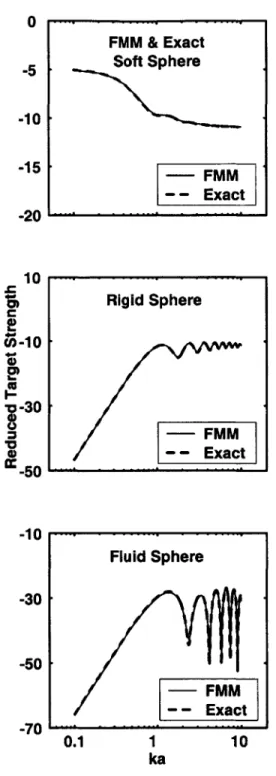
2.4.1 Spheres: comparison with exact solution . . . . 68

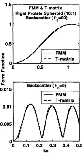
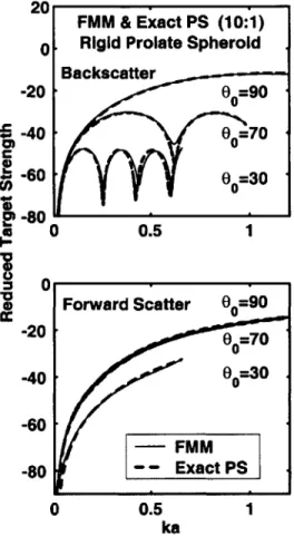
2.4.2 Prolate spheroids: comparison with various solutions . . . . 68

2.4.3 Irregular bodies: comparison with Kirchhoff approximation . . . 77

2.4.4 Low ka resonance scattering for gaseous bodies: comparison with T-matrix and exact prolate spheroidal solutions . . . . 81

2.5 Summary and conclusions . . . . 83

3 Broadband acoustic backscatter and high-resolution morphology of fish: Measurement and modeling2 ₈₅ 3.1 Introduction . . . . 85

3.2 T heory . . . . 93

3.2.1 D efinitions . . . . 93

3.2.2 Pulse compression . . . . 94

2

This chapter is based on an article submitted to the Journal of the Acoustical Society of America (Reeder et al, submitted).

3.2.3 Models .9

3.3 Experimental methods . . . . 3.3.1 Animals . . . . 3.3.2 Morphometry of animal shapes: 3.3.3 Acoustic data acquisition . . . . 3.4 Experimental results . . . . 3.4.1 Spectral domain . . . . 3.4.2 Time domain . . . . 3.5 Modeling and comparison with data. . 3.5.1 Relating scattering features to fi

3.5.2 Modeling the scattering . . . .

3.6 Summary and conclusions . . . . PCX 99 99 102 107 and CT scans. . . . . 113 . . . . 113 sh a . . . . 113 . . . . 121 natom y . . . . 121 . . . . 126 . . . . 131

4 Summary and conclusions

4.1 Modeling ...

4.2 Measurement and analysis ...

4.3 Recommendations for future work . . . . 4.4 Contributions of this thesis ...

134 134 136 138 139 95

Chapter 1

Introduction

1.1

Historical background for the use of sound in

underwater observations

The first significant experiment in underwater acoustics was conducted by Colladon and Sturm in 1826 in the waters of Lake Geneva, Switzerland. By striking a bell underwater while simultaneously setting off a flash of light from explosives above the water, an observer in a boat some distance away measured the time lapse between the flash of light and the arrival of the sound of the ringing bell underwater. Colladon and Sturm, in a single experiment, not only a established a good value for the speed of sound (c) in fresh water but simultaneously, and possibly unintentionally, demonstrated the fact that as light and sight are the primary means of assessing the world above water, sound is the method of choice to observe the underwater world. Water is opaque to light but is

transparent to sound which can travel great distances through the ocean and be detected at low frequencies even at megameter ranges (Baggeroer et al., 1994).

Medwin and Clay (1998) opine that acoustical oceanography (the use of sound to study oceanographic processes) got its start in 1912, with the sinking of the HMS Titanic. Within months of the tragedy, patents were filed for new sonar systems to detect the presence of large objects underwater using acoustic backscattering. In fact, within 20 years of the Titanic's sinking, sonar was being used for the detection of schools of fish. Since that time, the science of underwater acoustics has progressed and has been applied in many ways to study the ocean environment. Much interest continues in the study of how human-generated sound interacts with marine organisms, whether for the purpose of understanding how the sound affects marine mammal behavior or for the purpose of detecting and tracking marine organisms. Acoustic scattering from marine organisms is the focus of much research by a diverse number of individuals: the academic biologist/acoustician, the commercial fisherman, the fisheries manager and the military sonar engineer.

1.2

Current interest in ocean observation

Just as in the 1930's, the modern commercial fisherman uses sonar to detect and localize the presence of schools of fish to maximize the catch. Given the limits on the number of fishing days and types of harvested fish allowed, remotely classifying fish would be advantageous for the commercial fisherman in order to avoid unnecessary catches of

unwanted species and to maximize time at sea by limiting operational costs in terms of payroll and fuel.

The fisheries manager is tasked with observing and estimating fish populations in particular regions of the ocean to prevent over-fishing and the resultant collapse of the fisheries as happened in New England (Fogerty and Murawski, 1998; Steele, 1998), or worse, the extinction of particular species due to over-fishing or habitat destruction.

The academician is interested in better understanding the distribution, diversity, abundance and size distributions of fish populations in order to assess the state of the resources present in the ocean and changes in the environment in which these organisms live. Without knowledge of these factors, it is difficult to determine, much less predict, the effect on populations of low availability of food supplies for each species or the effect of over-fishing by humans.

The military sonar engineer is interested in observing and understanding how sound interacts with boundaries such as the sea surface, the seafloor, turbulence, internal waves, bubbles and marine organisms. Organism-based sound can be due to scattering from the animal or actually produced by the animal itself, e.g., whales, dolphins and snapping shrimp (Au and Banks, 1998; Olivieri and Glegg, 1998; Versluis et al., 2000; Schmitz et al., 2000). For active sonar systems seeking an acoustic target, organism-based interference contributes to the background reverberation detected by the sonar, decreasing the signal-to-noise ratio (SNR) and lowering the probability of detection (Urick, 1983).

1.3

Methods of ocean observation

Historically, scientists have relied on ocean surveys involving direct sampling with various types of nets to assess organism populations. Direct sampling furnishes biological data like abundance, biomass, length and species identification but is time-consuming and expensive. The catch may not be representative of the biomass in the water column since the net is selective, and as many marine organisms are free swimmers, the animals can avoid the net. Some delicate animals are destroyed by the nets, making it difficult to count the catch. The population estimate generated from the survey is susceptible to error since the sampling volume is small relative to the size of the region that is being surveyed. The abundance estimate from the small volume is then extrapolated to the whole, large region, causing errors to be propagated and amplified in the biomass estimate.

To overcome the problems and limitations plaguing the biological oceanographer and fisheries manager, the use of acoustic technology has made it possible to do rapid, high-resolution, broad-scale synoptic surveys of marine organisms (Gunderson, 1993). An acoustic survey would be less expensive by sampling the entire water column at a much faster rate, requiring less ship-time and labor while providing total coverage of the sur-veyed region. The acoustic survey is non-invasive, eliminating the problems of net avoidance and destruction of the organisms. The potential exists for the acoustic survey to produce high-resolution maps that can help advance understanding of aquatic com-munity compositions, predator-prey interactions and habitat utilization (Horne, 1998).

Acoustic sampling produces acoustic data, not biological data; therefore, the acoustic backscattered signal must be translated into meaningful biological information. Abun-dance estimates using echo sounders have been made for several decades; however, these estimates are quite often based on the assumptions that (1) the aggregation is composed of animals of a single size and species, (2) the echo energy is proportional to the product of the number of animals per unit volume and average backscattering cross section, and (3) the average backscattering cross section is relatively constant for a given size and species, implying variations in echo energy are related to variation in numerical density. Directly relating acoustic scattering strength to biomass can be an unreliable indicator of abundance. The scattering strength of an organism depends upon the anatomical features of the animal, which vary widely between species that may even be of the same individual size or biomass, introducing large errors in the abundance estimates (Foote, 1980; Stanton et al., 1994a). Dawson and Karp (1990) observed that fish at nearly hor-izontal aspect experienced approximately 10 dB target strength variations, apparently due to its swimming motion only. In an earlier study, Nakken and Olsen (1977) noted a 20 dB variation over time for a swimming Atlantic cod (Gadus morhua) at zero tilt angle.

Therefore, the goal of inverting acoustic scattering by marine organisms for mean-ingful biological information such as species, size and numerical density requires an un-derstanding of the scattering characteristics of each type of organism. In other words, solving the inverse problem requires a detailed knowledge of the forward problem of

predicting the acoustic scattering based on each animal's unique acoustic signature. In the case of the impact of reverberation on the performance of military sonar sys-tems, characterization of the complex reverberant properties of the water column has been largely ignored, i.e., the physics of the scattering by inhomogeneities, and specifi-cally, marine organisms has not been taken into account in any significant way. Detailed physics-based characterization of marine organisms' scattering properties over a wide range of frequencies could lead to improvements in sonar system performance.

1.4

The physics of acoustic scattering

In order to exploit the properties of sound transmission and interaction with boundaries in the ocean, the physics of the scattering must be formalized and the factors affecting scattering studied in detail.

The far-field scattered sound wave is expressed as:

Psc -I Pinc

f

(1.1)

r-oo r

where pifc is the pressure amplitude of the incident acoustic wave upon the object

at a distance r away, k (= 2-r/A, A =wavelength) is the acoustic wavenumber of the incident field and f is the scattering amplitude. Given the dynamic range of the far-field scattering amplitude in the backscatter direction, it is often expressed in logarithmic terms as target strength (TS), expressed in units of decibels (dB) relative to 1 m (Urick,

1983):

TS = 10logo bs, (1.2)

where Ub, is the differential backscattering cross section, which can be considered to

be a measurement of the effective (acoustic) area of the target. The equation can be represented in another form:

TS = 20 logo IfbsI, (1.3)

where fb, is the backscattering amplitude and Os, = fb, 2.

The scattering amplitude,

f,

Prediction of an organism's scattering properties requires detailed, accurate measure-ment of the acoustic scattering characteristics of the animal of interest as well as a detailed theoretical scattering model to quantify the nature and extent to which size, shape, mate-rial properties, orientation and frequency affect scattering characteristics (Greenlaw and Johnson, 1983).

1.5

Overview of relevant work

Two vast bodies of literature exist on acoustic scattering that are nearly independent of each other: one consists of general scattering research without specific application,

while the other consists of studies on scattering by marine organisms specifically. Since the objective of this thesis is to contribute to both of these fields of study, the following paragraphs provide an overview of work done in both areas and a description of the factors that contribute to the complexity of scattering physics.

1.5.1

General scattering

Solutions to the wave equation can be approached in a number of different ways. Pos-sible approaches can be categorized as exact analytical, exact numerical or approximate methods of solution.

Exact analytical solutions to the wave equation require the scatterer surface to ex-actly match the locus of all points for a constant radial coordinate. Such exact analytical solutions exist only for a limited number of simple geometries (eleven) for which the sep-aration of variables is possible (Morse and Feshbach, 1953; Bowman et al., 1987). These exact analytical solutions are limited to smooth, simple geometries, such as the sphere, infinitely long cylinder, or spheroid. Exact analytical solutions for acoustic scatter-ing was first investigated in the 1870's by Lord Rayleigh (1945), where he considered the case of spherical and infinitely long cylindrical scatterers whose cross sections were small compared to the wavelength of the incident sound. Anderson (1950) presented an exact solution for scattering from a fluid sphere. Scattering by solid, rigid spheres and cylinders was investigated by Morse (1981), as well as Faran (1951) who focused on shear waves of the object. Junger (1951) formulated scattering from thin elastic,

air-filled shells of spherical and cylindrical shape in terms of "rigid body scattering" and "radiation scattering". Goodman and Stern (1962) addressed the problem of scattering by elastic spherical shells in which the material properties of the surrounding medium and the interior of the shell differ from the shell itself. Since scattering from simple spherical and infinitely long cylinders is not sufficient to describe scattering from realis-tic scatterers found in nature, scattering by prolate spheroids has been investigated by Spence and Granger (1951), Weston (1967), Yeh (1967), Furusawa (1988) and Ye et al. (1997). Some of these exact modal series solutions were transformed through use of the Sommerfeld-Watson Transformation to obtain an exact formulation for the rays scattered by bodies (Uberall, 1966; Williams and Marston, 1985).

Exact numerical solutions to the wave equation are required, particularly at high fre-quencies, once the scatterer shape deviates from a simple geometry, as do most realistic scatterers of interest. These formally exact, numerically solved methods include the per-turbation method (Ogilvy, 1991) which is limited to shapes that are close to a separable geometry, the T-matrix method (Waterman, 1968; Varadan et al., 1982; Lakhtakia et al., 1984; Hackman and Todoroff, 1985) and solving the boundary integral equation by the boundary element method (Tobocman, 1984; Francis, 1993). These numerical models are limited in that they can be computationally intensive and numerically unstable as the frequency or irregularity of the surface increases.

Approximate solutions are useful in that they provide an analytical solution under certain conditions of validity in which no exact solution exists, or they attempt to avoid

unwieldy analytical formulations or numerical difficulties inherent in the numerical im-plementation of exact solutions. Approximate analytical solutions include the physi-cal optics, or Kirchhoff, approximation (Born and Wolf, 1999; Neubauer, 1963; Junger, 1982; Gaunaurd, 1985) which involves an integral over the scatterer surface, the Born ap-proximation (Born and Wolf, 1991) and Distorted Wave Born Apap-proximation (DWBA) (Stanton et al., 1993; Chu et al., 1993) which involve an integral over the volume of the scatterer and the deformed cylinder method (Stanton, 1988a, 1988b, 1989a, 1989b) which involves a line integral. Other approximate solutions include the geometric theory of diffraction (Levy and Keller, 1959; Yamashita, 1990) which is based on the superpo-sition of scattered rays, as well as a ray solution for curved edges based on the exact solution for straight edges (Svensson et al., 1999). Approximate analytical solutions also include asymptotic formulations based on the exact solutions for the cases of low and high frequencies (Sammuelmann, 1988). While each of these approximations may perform well in their respective ranges of validity, they are all limited in one or more of the following conditions: frequency range, class of surfaces, types of boundary conditions and eccentricity of shape.

1.5.2

Scattering from marine life

In the particular field of acoustic scattering by marine organisms, the multitude of dif-ferent species of zooplankton and fish that occupy the water column make it impractical to study and acoustically characterize each individual species. Figure 1-1 illustrates the

categorization by gross anatomical structure and the approximation by simpler shapes necessary to describe the important scattering mechanisms of the animals. The great complexities of the physics of the scattering require detailed measurements and develop-ment of models to accurately characterize scattering from marine organisms.

Acoustic measurements of fish

Much research has been conducted to quantify, in terms of target strength, the efficiency with which fish scatter sound (Midttun, 1984). Studies include measurement of target strengths in situ and ex situ, with multiple and single targets. In situ measurements are conducted in the natural environment yet present the challenge of unknown target size, orientation and position relative to the acoustic beam; ex situ measurements, how-ever, provide greater control over these factors (Foote, 1997). Ex situ measurements of tethered fish (similar to the method presented in Chapter 3 of this thesis) include those conducted by Jones and Pearce (1958), Haslett (1969, 1977), Diercks and Goldsberry (1970), Love (1969, 1970, 1971), and Nakken and Olson (1977). In spite of the fact that these measurements were performed at a limited number of angles of orientation (mostly dorsal), they were performed on a variety of species of different sizes and at a number of different frequencies and demonstrate complicated variability that is dependent upon morphology, orientation and acoustic wavelength.

(a) Fl ~ BI nce field Incident field (b) 4- "Winged" foot -4- Opercular opening 4 Hard elastic shell Incident field fI f-L __~ (c) Gas inclusion Incident field fISSUE Tissue (nectophores, gastrozooids, etc) (d) _Incident field fSK SB

Skull Swim bladder

Figure 1-1: Several anatomical groups of zooplankton and fish, and certain important scattering components: (a) fluid-like, (b) elastic-shelled, (c) gas-bearing zooplankton, and (d) gas-bearing (swimbladder) fish. The scattering amplitude from the various anatomical features is indicated by an

f(...).

~~AS

4-Modeling scattering from fish

Attempts have been made to empirically quantify the relationship between echo ampli-tude and actual fish length (Love, 1977; Foote, 1987). Although linear regression curves have been used with some success, they are constrained to certain frequencies and species, and by the system's ability to acoustically resolve individuals within aggregations (Horne and Jech, 1999). More sophisticated scattering models are required to better account for the complexities introduced by shape, orientation and material properties. As mentioned earlier, the existence of numerous species with different shape and material properties

requires some simplification in the modeling.

For low frequency applications, the acoustically dominant swimbladder has been mod-eled as a sphere (Andreyeva, 1964; Love, 1978; Ye and Farmer, 1994; Feuillade and Nero, 1998) and as a prolate spheroid (Weston, 1967; Ye, 1996). Scattering from simple spheri-cal shapes is not sufficient to describe scattering from animals with more irregular shapes, particularly at high frequencies. Efforts have been made to describe the scattering by more realistic, elongated shapes. For example, Clay (1991) modified Stanton's (1988a, 1989a) deformed finite cylinder model and derived a ray-mode model for fish using a combination of gas- and fluid-filled cylinders.

Including the exact shape and size of the dominant scattering components of the animal is a crucial, yet very difficult aspect of building an accurate backscattering model. Modeling of the scattering of sound by complex body shapes is a difficult problem due to the mathematical challenge of exact solutions and the computational difficulties of

numerical approaches, as mentioned above. A number of approaches have been used to more closely represent the exact shape of the dominant scattering mechanisms. Arrays of point scatterers (Clay and Heist, 1984) have been used to model the fish body form. Clay (1991) developed the Kirchhoff ray-mode (KRM) model of finite cylinders that combines a modal solution for ka < 0.15 and a Kirchhoff approximation for ka > 0.15 to take advantage of the performance of the two models as a function of ka. Note that ka is a non-dimensional form of frequency, and a is the radius of the cylinder. Clay and Horne (1994) modeled acoustic backscatter of Atlantic cod (Gadus morhua) using the KRM model. Do and Surti (1990) used a series of cylinders and cones similar in concept to the KRM. Jones and Pearce (1958) and Haslett (1962b) attempted to experimentally approximate the shape of a fish swimbladder as a cylinder and ellipsoid, respectively. Foote (1985) computed the target strength of fish by applying the Kirchhoff approximation to a more realistic 3-dimensional model of the swimbladder based on the digitized microtomed swimbladder of pollack (Pollachius pollachius) and saithe (Pollachius virens). Foote and Francis (1999) modeled the target strength of swim-bladdered fish using the boundary element method based on the same swimbladder shapes in Foote (1985). Models using the exact shape of the animal's morphology are desired because they are more realistic and promise greater accuracy over models based on simple geometric shapes, especially in the geometric scattering region (high ka). As in the case of general scattering models, fish scattering models are generally limited with respect to frequency range, class of surfaces, types of boundary conditions, eccentricity of shape and/or numerical efficiency.

Complexities of scattering from marine life

Morphology

In the case of fish, morphology (size, shape and material properties) creates sound speed and density contrasts that have significant effect upon the scattering. Swimblad-ders have been considered to be the dominant scattering mechanism based on estimates that swimbladders cause as much as 90-95% of the target strength of fish under certain conditions due to the large acoustic contrast between the air-filled swimbladder and the surrounding tissue and water (Foote, 1980). Their influences on the acoustic signatures have been studied intensively by Jones and Pearce (1958), Andreyeva (1964), Weston (1967), Haslett (1962c), Hawkins (1977), Love (1978) and Foote (1980, 1985). While the size and shape of swimbladders may dominate the scattering properties of fish, other parts of the anatomy create acoustic impedance contrasts which contribute, particularly for fish without swimbladders, to the overall scattering, e.g., skull, vertebral column, muscle tissue and gonads. The extent to which each of these individual anatomical features contributes to the scattering from the whole fish is generally unknown, although some studies have illustrated their importance (Sun et al., 1985).

Orientation

Orientation has a profound effect upon scattering (Nakken and Olsen, 1977; Foote, 1985) at the higher frequencies. The effect of angle of orientation on scattering from the animal is further complicated by the movement of the animal during measurement (Zakharia, 1990). Slight movements of the animal in the laboratory setting reflect the

greater complexity of in situ measurements and acoustic surveys, where animal orienta-tion influences the received scattered signal.

Behavior and physiological changes

The physical parameters of morphology and orientation mentioned above are also influenced by behavior, further complicating the process of accurately measuring their acoustic properties. Those factors include depth excursions, swimming motion that changes aspect, ingesting and expelling of air to change buoyancy, size of the gut after feeding, seasonal effects such as spawning, and physiological effects such as voluntary

muscular tension on the swimbladder wall (Hawkins, 1981; Feuillade and Nero, 1998). Frequency

Generally, the scattering strength of a fish varies with frequency (Haslett, 1962a; Love, 1969, 1971). At very low frequencies in the Rayleigh scattering region, the backscat-tering cross section is proportional to the fourth power of frequency. At swimbladder resonance frequencies, backscattering cross section varies with fish size and frequency. In the geometric scattering region at higher frequencies, it depends on multiple scattering features in the fish which will cause interference in a manner specific to its anatomy, and that interference pattern is dependent upon frequency (Haslett, 1962c). In other words, the physical separation of scattering features in the fish relative to acoustic wavelength determines the interference pattern.

Broadband

at single frequencies. Although this level of information can be invaluable for fishery population estimates, traditional target strength measurements lack coherent information necessary for extracting more detailed information, such as size and species identification. Specifically, narrowband measurements are performed at discrete frequencies, thus fre-quency dependencies are missing from the data, although this has been addressed in part by use of multiple discrete frequencies. Since an animal's scattering properties vary con-siderably with the frequency of the transmitted signal, the use of broadband transducers would offer continuous coverage over a significant range of frequencies, thus increasing the amount of information contained in the signal. Furthermore, the broadband signals inherently have high temporal resolution (which varies with inverse bandwidth of the transmitted signal) which can be realized through the use of an impulse signal or pulse compression of a longer signal (Chu and Stanton, 1998). With high temporal resolution, scattering features can be realized in the time domain. In spite of the great advantages of broadband signals, relatively few studies have investigated the finer structure of the an-imal's spectral characteristics (Kjaergaard et al., 1990; Simmonds et al., 1996; Zakharia et al., 1996). Characterizing an animal's scattering properties over a broad bandwidth is made difficult by the lack of well-performing and affordable broadband transducers in the desired frequency ranges, but advances in the field are being made.

1.6

Purpose of this thesis

As demonstrated by the research outlined above, predicting and modeling the scattering of sound by irregular finite objects is formidable. Successful use of acoustics by the biologist, commercial fisherman, fisheries manager and military sonar engineer requires accurate scattering models for each category of object or animal, verification of the models through accurate measurements of scattering from those objects or animals, and reliable inversion algorithms.

In particular, a general acoustic scattering model is needed that is numerically efficient over a wide range of frequencies for all angles of orientation (three-dimensional), for realistic shapes and boundary conditions. In addition, high-resolution measurements of the morphology of fish are needed to accurately represent the exact shapes of the scattering features in the fish on which the models are based. Furthermore, high-quality acoustic backscattering measurements of fish are needed for the identification of dominant scattering mechanisms of fish and testing and refinement of the scattering models. The acoustic measurements need to be performed under the following conditions: (1) live, healthy fish in an environment that mimics their natural environment, (2) control of the position of the fish within the acoustic beam to allow measurements of target strength, (3) control of angle of orientation with high angular resolution, (4) measurements in more than one plane, and (5) the use of broadband signals to make possible spectral and time-domain processing techniques. The measurements, analysis and modeling presented in this thesis seek to meet these needs.

Chapter 2 of this thesis describes the development of an advanced acoustic scatter-ing model that can be used in a wide variety of applications, includscatter-ing scatterscatter-ing from fish. The scattering model is an extension to axisymmetric finite-length bodies of a two-dimensional general scattering model, called the Fourier matching method (FMM)

(DiPerna and Stanton, 1994). It involves conformally mapping the scatterer surface, which can be irregular, to a new coordinate system in which the locus of points describ-ing the radial coordinate bedescrib-ing a constant coincides with the scatterer surface. It is a numerically efficient solution that is valid for a wide range of frequencies, over all angles of orientation, for smooth and irregular surfaces, and all scalar boundary conditions.

Chapter 3 describes the experiment and analysis portion of the project. As outlined above, detailed knowledge of the morphology of fish is critical to gaining an accurate knowledge of its scattering properties. Two imaging techniques which are used to exactly measure the morphometry of the scattering features of fish include very high-resolution Phase Contrast X-rays (PCX) and Computerized Tomography (CT) scans, the images from which are incorporated into the FMM scattering model. The results of an extensive, high-quality set of broadband acoustic backscattering measurements conducted on alewife fish over a wide frequency band and over all angles of orientation (10 increments) in two planes of rotation are presented, including the use of both spectral and time-domain analysis techniques to extract unique features from the backscattering acoustic signals from the fish to aid the inference of its acoustic scattering characteristics.

contributions of the thesis, and recommendations for future work.

A final note about the format of this thesis is in order. Chapters 2 and 3 were writ-ten as manuscripts for submission to the Journal of the Acoustical Society of America and were, therefore, written as self-contained articles. Consequently, some discontinu-ity and redundancy in the thesis is unavoidable; however, such organization involving independent chapters benefits the reader who is interested in only a portion of the thesis.

Chapter 2

Acoustic scattering by axisymmetric

finite-length bodies:

An extension

of a 2-dimensional conformal

mapping method

1

2.1

Introduction

The prediction of acoustic scattering from finite and infinitely long bodies has been pursued for many years, starting with Lord Rayleigh's work on scattering from a sphere (Rayleigh, 1945). Exact analytical solutions to the acoustic wave equation require the 1_{This chapter is based on an article submitted to the Journal of the Acoustical Society}

scatterer's surface to exactly match the locus of all points for which the radial coordinate is a constant. Such exact analytical solutions exist only for a limited number of cases for which the separation of variables is possible (Morse and Feshbach, 1953; Bowman et al., 1987). In all of these cases, the boundary is simple; e.g., a sphere, infinitely long cylinder and prolate spheroid.

For complex shapes, approximate analytical solutions, including the perturbation method, and approximate asymptotic formulations, such as physical optics (Gaunaurd, 1985) and the geometric theory of diffraction (Levy and Keller, 1959; Yamashita, 1990) have been developed. Numerical solutions have also been developed, including the boundary element method (Tobacman, 1984; Francis, 1993), T-matrix (Waterman, 1968; Varadan et al., 1982; Lakhtakia et al., 1984; Hackman and Todoroff, 1985) and the mode matching methods (Yamashita, 1990). All of these approaches are limited in one or more of the following: frequency range, class of surfaces, types of boundary conditions, eccentricity of shape and/or computational implementation and numerical efficiency.

DiPerna and Stanton (1994) introduced a conformal mapping approach to predicting far-field sound scattering by infinitely long cylinders of noncircular cross section. The approach, termed the Fourier Matching Method (FMM), involves a conformal mapping of variables to a new coordinate system in which the constant radial coordinate exactly matches the scatterer surface. The method makes use of the Newton-Raphson algorithm to execute the mapping. The boundary conditions are satisfied by requiring the Fourier coefficients in the new angular variable of the total field to be zero and then the resultant

scattered field is expressed in terms of circular eigenfunctions.

The FMM proved to be accurate over a wide range of frequencies, shapes of cross sec-tion, and penetrable (fluid) as well as impenetrable boundary conditions. Furthermore, the approach is inherently numerically efficient due to the nature of its formulation. For example, the FMM was shown by DiPerna and Stanton (1994) to be more efficient than the T-matrix method for the case of the high-aspect-ratio elliptic cylinder because fewer terms were needed for the numerical integrations. Even after incorporating the FMM basis functions into the T-matrix calculations, the FMM required 85% fewer integration points.

A major limitation of the two-dimensional FMM was the fact that it was formulated for the case of an infinitely long cylinder-a two-dimensional scattering solution. Many practical scattering problems involve scattering from finite bodies and cannot be accu-rately modeled by the two-dimensional solution. In order to address this need, the FMM is extended in this paper to predict the scattering from finite-length bodies. In order for this particular approach to be used for finite bodies, the outer boundary of the bodies must be described by a function rotated about the length-wise axis. Hence, although the function is arbitrary and these bodies are three-dimensional, they are restricted to axisymmetric shapes. As with the two-dimensional formulation, this approach is in-trinsically numerically efficient and is valid over a wide range of frequencies and shapes as well as both monostatic and bistatic scattering geometries. The extension has been formulated for three boundary conditions-Dirichlet (soft, or pressure-release), Neumann

(rigid) and Cauchy (fluid). In all three cases, the surrounding material is fluid.

In Section II, the theoretical basis for the formulation is presented, which includes the development of the new orthogonal coordinate system to which the body is mapped, the conformal mapping procedure, modal series solutions to the transformed Helmholtz equation, and resulting equations for the modal series coefficients after satisfying the three boundary conditions. In Section III, several practical numerical issues that arise in the solution of the scattering problem are explored, including the effect of machine precision, truncation of the modal series, and the choice of numerical methods. In Section IV, the numerical results are presented for various shapes (spheres, smooth prolate spheroids and two finite bodies with irregular surfaces), boundary conditions (soft, rigid and fluid), and over a wide range of frequencies and scattering angles. The results are compared with various previously published results using other approaches. Section V contains a summary and concluding remarks.

2.2

Theory

The derivation of the extended formulation for scattering by an axisymmetric finite-length body is conceptually very similar to the corresponding derivation of the two-dimensional solution described by DiPerna and Stanton (1994); in fact, some of the elements are identical. Both solutions begin with the wave equation in a known coordinate system and conformally map the coordinate variables to a new, orthogonal coordinate system in which the locus of all points where the new radial coordinate is a constant exactly

coincides with the scatterer surface. The difference in the coordinate systems between the two cases concerns the fact that one involves two-dimensional coordinates while the other involves an additional coordinate dimension with a new geometry defined for the finite body. Both solutions use mapping functions that are identical in form, transform the Helmholtz equation to the new coordinate system, and then satisfy the boundary conditions using identical techniques to arrive at differing, yet structurally similar, ex-pressions for the scattered pressure. The two-dimensional solution includes a mapping function that corresponds to the shape of the boundary of a cross-sectional slice of the cylinder, while the three-dimensional solution uses a mapping function that corresponds to the shape of the boundary of a length-wise slice of the body (specifically, the function that is rotated about the longitudinal axis). Furthermore, the two-dimensional solution includes circular eigenfunctions while the three-dimensional solution for the scattered pressure is expressed in terms of spherical wave functions; i.e., spherical Bessel and Han-kel functions and associated Legendre functions. Due to these similarities, the original work will be referred to quite regularly in the development that follows.

Consider the scalar wave equation:

1 02P

V2_{P = -9} 2 _(2.1)

C2 190

where P(x, y, z) is the acoustic pressure in three dimensions, V2 is the Laplacian operator, c is the speed of sound, and t is time. Assuming a harmonic time dependence, eiwt, where w is the angular frequency, the wave equation becomes the scalar Helmholtz differential

equation in Cartesian coordinates:

V2_{P(x, y, z) + k}2_{P(x, y, z) = 0. (2.2)}

Here, k = w/c = 27r/A is the spatially independent acoustic wave number and A is the acoustic wavelength. In all cases considered here, the body does not support shear waves and is surrounded by a fluid medium. By a conformal (angle- and orientation-preserving) transformation of coordinates, the transformed Helmholtz equation in the new coordinate system becomes:

V2_{P(u, w, v) + k}2_{F(u, w)P(u, w, v) = 0, (2.3)}

where (u, w, v) are the new coordinates, and F(u, w) is a function which depends on the specific transformation (Morse and Feshbach, 1953; DiPerna and Stanton, 1994). With the exception that the wave number is now a function of position, the new Helmholtz equation is formally identical to the Helmholtz equation in Cartesian coordinates.

2.2.1

Conformal mapping

Since x, y and z are mutually orthogonal in the Cartesian coordinate system, conformally mapping them into a new coordinate system guarantees that the new coordinates (u, w, v) will be mutually orthogonal, which eases the computation of the normal particle velocity on the boundary. Additionally, the conformal mapping generates a new set of angular

functions which fit the scatterer surface more naturally; that is, points along the surface that change rapidly in (x, y, z) are sampled at a higher spatial rate yet are equally spaced in (u, w, v). A new coordinate system must first be established, and then the conformal mapping function is defined and expanded to provide a method by which the body may be mapped to the new coordinate system.

Orthogonal coordinate system

An orthogonal coordinate system can be generated for a three-dimensional body of rev-olution from a two-dimensional conformal mapping. Consider the geometry in Fig. 2-1, in which

#

#

x

= (0, 2n) U=O

v =(0, 2n) r(u, i) ,w= (0, n)

g(u, )

Figure 2-1: Scattering geometry for an irregular, axisymmetric finite-length body. The body is symmetric about the z-axis. The azimuthal angular coordinates, < and v, range from 0 to 27r in the xy-plane, and the polar angular coordinates, 0 and w, range from 0 to

7r, measured from the z-axis. The radial coordinate in the (u, w, v) coordinate system

equals zero on the surface. Broadside incidence corresponds to 0=90 degrees. End-on incidence corresponds to 0 and 180 degrees. In the new coordinate system, g(u,w) is the length along the z-axis, and f(u,w) is the projection in the xy-plane.

f

2-1, trigonometry

x(u, w, v) = f (u, w) cos(v) (2.4)

y(u, w, v) = f(u, w) sin(v) (2.5)

(2.6) z(u, w, v) = g(u, w).

The position vector, 7, is defined in the new coordinate system by:

7

wherei,

j,

7

The local projection of

7

7

7,,

r = fW(u, w) cos(v)i + fw(u, w) sin(v)j + gw(u, w)k

(2.9)

= -f(u, w) sin(v)i + f (u, w) cos(v)j, (2.11)

where the subscript denotes the variable with respect to which the partial derivative is taken.

As mentioned earlier, an orthogonal coordinate system is desirable since it facilitates the computation of the normal particle velocity on the boundary necessary for satisfying the boundary conditions, and more naturally fits the scatterer surface. An orthogonal coordinate system requires the following condition to be satisfied:

r u r = 0 (2.12)

r w r = 0 (2.13)

r. . = 0, (2.14)

which can be expanded as:

fu(u, w)f(u, w) cos(v) sin(v)(-1 + 1) = 0 (2.15)

f (u, w)f (u, w) cos(v) sin(v)(-1 + 1) = 0 (2.16)

The first two conditions are automatically satisfied. The third condition simplifies to:

fM(u,w)fW(u, w) + gu(u, w)gw(u, w) = 0, (2.18)

which will be satisfied if:

fu(u, w) = gw(u, w) (2.19)

and

fW(u,w) = -gu(u, w). (2.20)

These are precisely the Cauchy-Riemann equations for an analytic function (Hildebrand, 1964). Therefore, if f(u, v) and g(u, v) are chosen to be harmonic, then the Cauchy-Riemann conditions will be satisfied, making them analytic functions which represent a conformal transformation. A shape initially plotted in the (x, y, z) coordinate system will be transformed into a shape in the (u, w, v) coordinate system with changes in position and size while preserving angles and proportions (Morse and Feshbach, 1953). Orthogonality of the coordinate system as well as the form of the Helmholtz equation will be preserved (Strang, 1986).

Mapping function

As discussed above, a conformal mapping function must be developed to map the scat-terer from the old coordinate system to the new orthogonal, axisymmetric coordinate system just developed. It must be noted at this point that, to the authors' knowledge, a

general three-dimensional mapping does not exist in the field of mathematics. Due to the fact that conformal mappings are currently limited to two dimensions, the geometry for the finite body must be axisymmetric about one of the axes, using the two-dimensional function that is to be conformally mapped to form the body by revolution about the axis. The particular mapping used herein is a two-dimensional mapping developed by DiPerna and Stanton (1994) extended to a finite body of revolution which is axisymmetric about the longitudinal axis. The infinitely long cylindrical geometry in DiPerna and Stanton (1994) was described in circular cylindrical coordinates with the radial coordinate, r, being a function of 9, the azimuthal angular coordinate ranging from 0 to 27r. The conformal mapping in that case applied to the function, r(0), which corresponded to the shape of the boundary of a cross-sectional slice. In this work, 0 is now the polar angular coordinate ranging from 0 to ir, and <$ is the azimuthal angular coordinate ranging from 0 to 27r. The function, r(9), and associated conformal mapping is now associated with the shape of the boundary of a length-wise slice.

The category of surfaces described by Eqs. (2.4)-(2.6) has the additional limitation that r be single-valued; i.e., there can be only one value of r for each w. Following DiPerna and Stanton (1994), the mapping procedure for the axisymmetric finite body is commenced by expanding r in a Fourier series relative to the polar angle, 9, shown in Fig. 2-1:

r(9) = a + [r cos(nO) + r' sin(nO)], (2.21)

n=1

coefficients that in this case correspond to the deviation of the surface from the shape of a circle. Note that the series requires more terms to converge for a high aspect ratio

(ratio of length to width) prolate spheroid compared to the Fourier series for a shape that varies little from the shape of a circle. Rewriting the cos(nO) and sin(nO) functions in terms of exponentials and using the expression:

1

Rn =-[r' + ir'], (2.22)

2n n

gives

00

reO = aeiO + [R*ei+n)O + &ei(1-n)O] (2.23) n=1

For a conformal mapping from the (x, y, z) coordinate system to the new coordinate

system in (u, w,v):

M(p) = M(u + iw), (2.24)

where M(p) is the analytic mapping function in terms of u, the radial variable, and w, the polar angular variable, and p is the distance between the axis and outer boundary (i.e., the radius of a given cross-sectional slice). It is desirable to make scattering predictions using this model without inversely mapping the results of this model back to the original coordinate system. The potentially difficult inverse mapping is avoided by choosing M(p) such that the coordinate system becomes spherical as the radial coordinate is increased. While the choice of such a mapping function allows predictions of this model to be easily compared to existing solutions, it restricts direct comparisons to the

far-field. The general approach can certainly be used in the near-field, but comparisons of near-field scattering between this formulation and other solutions would require an inverse mapping. Note also that there will be two different mapping functions: G(p) for the exterior problem and T(p) for the interior problem. For the interior problem, T(p) is chosen such that the coordinate system becomes spherical as the radial coordinate is

decreased.

For the exterior problem, G(p) must be chosen such that:

(1) As u -* _{oo, the coordinate system becomes spherical,}

(2) the transformed Helmholtz equation is solvable, and (3) u = 0 is the scatterer surface.

The first two conditions can be satisfied by choosing the form of the exterior mapping function (DiPerna and Stanton, 1994) to be:

G(p) = ceP + Ce-"P (2.25)

n=O

which can be decomposed into the complex components:

g(u, w) Re(G(p)) = cleu cos(w) + E ce-" cos(nw) (2.26) n=O

and

f(u, w)

scatterer surface in the new coordinate system. Setting the surface, as represented in the two coordinate systems, equal to one another with u = 0 gives:

00

G(p)I=o = c-iew + Zcne-i", (2.28)

n=O

and substituting further from Eq. (2.23):

00 00

aeiO + Z[R*ei(1+n)O + ne'(1-nO ceiW + c ine . (2.29)

n=1 n=O

Since the left-hand side contains positive and negative frequency components while the right-hand side contains only negative frequency components (with the exception of c_1eiw), 0 and w are not equal; therefore, it is necessary to determine the extent to which 9 depends on w. Since it was assumed earlier that the surface is periodic and can be represented as a Fourier series, the deviation of 9 from w will be periodic and can be represented as a Fourier series. Specifically, assume:

00

9(w) = w + Z[6'cos(lw) + 6'sin(lw)]. (2.30)

1=1

The conformal mapping relies on the choice of 6' and 6' such that Eq. (2.29) is satisfied. Using the orthogonality relationships of complex exponential functions, multiplying both

sides by (1/27r)e-iiw and integrating over w from 0 to 27r:

e-i aeO() + Z[R*ei(1+n)o(w) + Rnei(1n)9(w)] dw =

(2.31) where

j

The uniqueness of the transformation is tested by verifying that the Jacobian of the transformation is nonzero. This ensures that there exists only one (x, z) for each (u, w). Specifically:

IG'(p)1

The interior mapping procedure is identical to the exterior mapping procedure with the exception that the interior mapping function, T(p), is different from G(p); specif-ically, T(p) is chosen such that the coordinate system becomes spherical as the radial

coordinate is decreased. The remaining two conditions mentioned above in the choice of G(p) remain the same for the interior problem. These conditions are satisfied by:

T(p) = Ztne"P. (2.33)

n=O

To summarize, the procedure described above to conformally map the scatterer shape from the original coordinate system to a new coordinate system is identical in form to the procedure presented in DiPerna and Stanton (1994). In this study, the same mapping procedure is extended to a different (finite-length, axisymmetric) scattering geometry; specifically, it is extended to the shape of the boundary in the length-wise slice. The results of this mapping will be used in solving the Helmholtz equation in three-dimensions in the next section.

2.2.2

Solutions to the Helmholtz equation

The 3-dimensional Helmholtz equation from Eq. (2.2) in spherical coordinates is:

the general solution to which is:

00 00

pext(r, 0,) = E anmjn(kr)Pn (cos(0))eim (2.35)

n=-oo m=-oo

+ bnmh$')(kr)P, (cos(9))emI,

n=-oo m=-oo

where j(kr) is the spherical Bessel function of the first kind of order n, h$((kr) is the

spherical Hankel function of the first kind of order n, and Pn(cos(9)) is the associated

Legendre function of degree n and order m. The radial coordinate is r, the polar

angular coordinate is 0, and the azimuthal angular coordinate is 4. The scattered field

coefficients, bnm, are to be determined by satisfying the boundary conditions using the

known coefficient, anm, of the incident plane wave field traveling from the 0 direction:

anm = inE(2n + 1)fn + 1 P"(cs(0)), (2.36)

IP(n + m + 1)

where em is the Neumann factor, P is the gamma function, and 0 is the angle of incidence of the incident wave relative to the z-axis.

Pe-t(r, 0,

#)

II.A.1 and Fig. 2-1: