HAL Id: hal-00734361
https://hal.archives-ouvertes.fr/hal-00734361
Submitted on 20 Apr 2018HAL is a multi-disciplinary open access archive for the deposit and dissemination of sci-entific research documents, whether they are pub-lished or not. The documents may come from teaching and research institutions in France or abroad, or from public or private research centers.
L’archive ouverte pluridisciplinaire HAL, est destinée au dépôt et à la diffusion de documents scientifiques de niveau recherche, publiés ou non, émanant des établissements d’enseignement et de recherche français ou étrangers, des laboratoires publics ou privés.
Fluorescence properties of dissolved organic matter in
coastal Mediterranean waters influenced by a municipal
sewage effluent (Bay of Marseilles, France)
Marc Tedetti, Rachele Longhitano, Nicole Garcia, Catherine Guigue, Ferretto
Nicolas, Madeleine Goutx
To cite this version:
Marc Tedetti, Rachele Longhitano, Nicole Garcia, Catherine Guigue, Ferretto Nicolas, et al.. Fluores-cence properties of dissolved organic matter in coastal Mediterranean waters influenced by a municipal sewage effluent (Bay of Marseilles, France). Environmental Chemistry, CSIRO Publishing, 2012, 9 (5), pp.439-448. �10.1071/EN12081�. �hal-00734361�
Fluorescence properties of dissolved organic matter in coastal Mediterranean waters influenced by a municipal sewage effluent (Bay of Marseilles, France)
M. Tedetti*, R. Longhitano, N. Garcia, C. Guigue, N. Ferretto, M. Goutx
Aix-Marseille Univ., Mediterranean Institute of Oceanography (MIO), 13288, Marseille, Cedex 09, France ; Université du Sud Toulon-Var, MIO, 83957, La Garde cedex, France ; CNRS/INSU, MIO UMR 7294; IRD, MIO UMR 235.
*
Corresponding author: marc.tedetti@univ-amu.fr; Phone: + 33 4 91 82 90 62; Fax: + 33 4 91 82 90 51
Final version
Environmental Context. Marine dissolved organic matter plays a key role in the global carbon cycle. Questions remain, however, as to the influence of anthropogenic activities on its composition and distribution in coastal waters. We studied dissolved organic matter in coastal waters influenced by a municipal sewage effluent (Marseilles City, France). We found that dissolved organic matter in the vicinity of the sewage effluent contained a high proportion of protein-like material. Hence, we demonstrate the influence of human activities on coastal dissolved organic matter.
ABSTRACT
We characterized fluorescent dissolved organic matter (FDOM) in coastal marine waters influenced by the municipal sewage effluent (SE) from Marseilles City (France, northwestern Mediterranean Sea). Samples were collected eleven times from September 2008 to June 2010 in the Bay of Marseilles along a coast-open sea transect from the SE outlet in the South Bay and at the Mediterranean Institute Observation site in the central Bay. Fluorescence
excitation-emission matrices (EEMs) combined with parallel factor analysis (PARAFAC) allowed the identification of two protein-like (tyrosine C1, λEx/λEm: < 230, 275/306 nm; tryptophan C2, λEx/λEm: < 230, 270/346 nm) and three humic-like components (marine humic C3, λEx/λEm: 280/386 nm; C4, λEx/λEm: 235, 340/410 nm; C5, λEx/λEm: 255, 365/474 nm). From the SE outlet to the central Bay, a gradient appeared, with decreasing FDOM intensities, decreasing dissolved organic carbon, particulate carbon, nutrients and fecal bacteria concentrations, and increasing salinity values. This gradient was associated with decreasing abundances in protein-like fluorophores and rising abundances in humic-like (C3 and C5) materials. This shift in FDOM composition illustrated the decrease in wastewater inputs and the increase in marine sources of DOM along the transect. FDOM data showed that the Marseilles SE spread up to 1500 m off the outlet while it did not reach the central Bay.
Tryptophan-like material was the dominant fluorophore in the SE and displayed the highest correlations with biogeochemical parameters (organic carbon, phosphates, fecal bacteria). Therefore, we propose to use its fluorescence intensity to detect and track SE inputs in the Marseilles coastal marine waters.
Keywords: EEM fluorescence; PARAFAC; sewage effluent; Mediterranean Sea; Cortiou; tryptophan
Introduction
Dissolved organic matter (DOM), which represents one of the largest active pools of organic carbon at the earth’s surface (~ 700 Gt C), plays a key biogeochemical role in the aquatic medium.[1-3] Fluorescence spectroscopy techniques, in particular excitation-emission matrices (EEMs), have been successfully used to investigate the origin, distribution and dynamics of DOM in various marine and freshwater environments.[4] EEMs, coupled to peak picking technique or to parallel factor analysis (PARAFAC), have allowed the identification of two main types of fluorophores within the aquatic DOM pool: 1) the protein-like
fluorophores, with fluorescence signatures roughly similar to those of tryptophan and tyrosine aromatic amino-acids, generally attributed to autochthonous/labile DOM and 2) the humic-like fluorophores, with fluorescence signatures corresponding to those of humic and fulvic acids, rather associated with terrestrial/degraded DOM.[5-8]
The discharge of sewage effluents (SEs) in the aquatic systems is a source of
environmental concern for a long time and will continue to be a major problem in future years due to the population growth and increasing urban activities combined with the effects of climate change such as unpredictable rainfall patterns.[9] SEs may contain high levels of organic matter, nutrients, fecal bacteria, viruses and chemical contaminants such as heavy metals, hydrocarbons, pesticides, polychlorinated biphenyls and pharmaceutical products. [10-12]
Interestingly, EEMs and synchronous fluorescence spectroscopy have proven to be relevant tools for tracking and fingerprinting SE-derived DOM in rivers and estuaries.[13-15] Indeed, the rivers impacted by treated/untreated SEs generally show higher tryptophan-like/humic-like fluorescence ratios compared to “clean” rivers.[16] In the latter, DOM mostly originates from terrestrial plants and soils, and thus contains a high amount of humic-like fluorophores and a low content in protein-like substances.[4,7] In contrast, DOM derived from
SEs is enriched in tryptophan-like fluorophore,[17-19] ascribed to high levels of microbial activity in the effluents.[20-22] However, although numerous studies have already investigated the fluorescent DOM (FDOM) composition in municipal/industrial/agriculture SEs[19,22-24] or in SE-impacted rivers/estuaries,[13-15,25-27] much less work has focused on the FDOM
distribution in coastal marine waters influenced by diverse SE inputs.[28-30] Noneof them addressed the Mediterranean Sea.
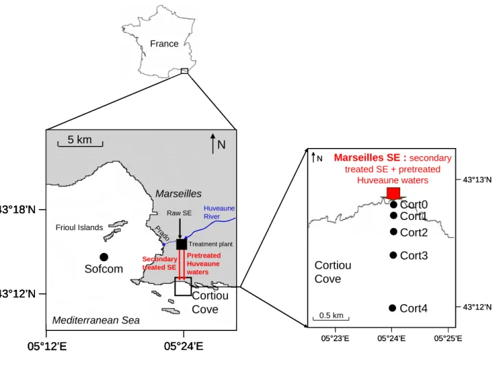
Located 8 km east from Marseilles City (northwestern Mediterranean Sea, France), Cortiou Cove is the discharge area of the municipal SE from Marseilles and fifteen
surrounding municipalities. The latter (termed “Marseilles SE”) is composed of a secondary-treated SE and presecondary-treated river waters. Despite the establishment of primary (physico-chemical) and secondary (biological) wastewater treatments in 1987 and 2007, respectively, Cortiou Cove is still considered one of the most polluted coastal sites of the French
Mediterranean.[31-34] The aim of this study is to characterize the FDOM pool in the marine waters influenced by the Marseilles SE using EEM spectrofluorometry and PARAFAC modelling. We report a time-series of FDOM data, associated with environmental parameters, collected in the Bay of Marseilles from September 2008 to June 2010.
Materials and methods
The Marseilles sewage effluent
The Marseilles SE is released in the surface waters of Cortiou Cove (Fig. 1). It is composed of 1) a secondary-treated SE (domestic sewages with or without storm waters) and 2) the pretreated Huveaune River waters. In dry weather, the secondary-treated SE contains
am (1.3 m3 s-1) and maximal at 10:30 am (3.2 m3 s-1), the secondary-treated SE flow rate is directly linked to the daily activity patterns of the urban population. The SE residence time inside the treatment plant is ~ 4 h [data from the Société d’Exploitation du Réseau
d’Assainissement de Marseille (SERAM)]. During rain events, the SE flow rate significantly rises due to the input of storm waters. Above 12 m3 s-1, the Marseilles treatment plant cannot process the SE anymore, which is directly discharged (untreated) into the sea. Since 1981, the Huveaune River, the main river of Marseilles, is routinely diverted from its natural outlet towards the treatment plant, pretreated, and transported to Cortiou Cove through the same sewer as the secondary-treated SE (Fig. 1).
In Cortiou Cove, the extent and fate of the Marseilles SE plume depends on its flow rate and on local hydrodynamic conditions. The latter are controlled by 1) the general circulation of the northwestern Mediterranean Sea, with the North Current that flows along the
continental slope towards the west, 2) the wind-induced circulation and 3) the complex bathymetry of the Cortiou area and the shallow depths of its western part. Under low wind speed conditions, the dilution plume may persist up to 1500 m from the outlet with a
westward-curved structure (influence of the North Current).[32] With southeast wind events, the dilution plume is pushed to the west coast, whereas under north wind conditions it extends offshore or eastward.[35] At the outlet, the plume presents a low salinity over a thickness of 3-4 m while this low salinity is observed over only few centimeters around 1 km from the outlet.[32] The residence time of waters from Cortiou Cove is approximately 2 days.[36]
Study sites and sampling
Seawater samples were collected eleven times from September 2008 to June 2010 in the Bay of Marseilles (northwestern Mediterranean Sea) aboard the R/V Antédon II. Five stations were sampled in the Cortiou area (South Bay) along a coast-open sea transect: Cort0 (40 m
from the outlet), Cort1, Cort2, Cort3 and Cort4 (1500 m from the outlet). An additional site was sampled away from Cortiou Cove: Sofcom, the observation station of the Mediterranean Institute, located in the central Bay near Frioul Islands at 7 km from the coast (Fig. 1; Table 1). The sampling was performed in the morning, between 9:30 and 11:00 am for Cortiou stations (i.e. at or close to the maximal secondary-treated SE flow rate) and between 11:00 and 12:00 am for Sofcom, in dry weather under a variety of wind and sea conditions.
Samples were taken in the subsurface water (SSW) at ~ 0.1 m depth using Nalgene® polycarbonate bottles. The bottles were opened below the water surface to avoid the sampling of the surface microlayer. At Sofcom and Cort4, samples were also collected at 5, 20 and 55 m depth using a 5 l Niskin bottle equipped with silicon ribbons and Viton o-rings (Table 1). The bottles were washed with 1 M hydrochloric acid (HCl) and ultrapure water (i.e. Milli-Q water, final resistivity: 18.2 MΩ cm-1) before use, rinsed three times with the respective sample before filling and stored in the dark in the cold.
Along with the discrete water samples, profiles of temperature (T), salinity (S) and chlorophyll a (Chla) concentration were obtained from a Seabird Electronics 19plus
conductivity temperature depth (CTD) profiler equipped with a WETStar Chla fluorometer (WETLabs, Inc).
Filtration and handling of samples
Back in the laboratory, the samples were immediately filtered under a low vacuum (< 50 mm Hg). Filtration of samples was performed about 2-3 hours after their collection. The samples for FDOM and dissolved organic carbon (DOC) measurements were filtered through 0.2 µm polycarbonate filters (25 mm diameter, Nuclepore) in small pre-combusted (450 °C, 6 h) glass filtration systems. Prior to sample filtration, Nuclepore filters were first soaked in 1
sample. The 0.2 µm filtered water was transferred into pre-combusted 10 ml glass tubes (FDOM) and ampoules (DOC). The ampoules were flame-sealed after addition of 10 µl of 85% phosphoric acid. FDOM and DOC samples were kept at 4 °C in the dark during 24-48 h until analyses. The samples for particulate carbon (PC) measurements were filtered through GF/F glass fiber filters (47 mm diameter, Whatman). The GF/F filters were then dried 24 h at 50 °C and stored in a vacuum dryer until analysis. The samples for nutrients were analysed without being filtered. The samples for nitrate (NO3-), nitrite (NO2-) and phosphate (PO43-) determination were collected into 50 ml polyethylene flasks and stored frozen until analysis.
Analysis of fluorescent dissolved organic matter (FDOM)
Instrument. FDOM measurements were carried out using a Hitachi F-7000
spectrofluorometer (Japan). This instrument, which provides a measuring wavelength range of 200-750 nm on both Ex and Em sides, is equipped with a 150 watt xenon short-arc lamp with a self-deozonating lamp compartment as light source, two stigmatic concave diffraction gratings with 900 lines mm-1 brazed at 300 (Ex side) and 400 nm (Em side) as single monochromators, and Hamamatsu R3788 (185-750 nm) photomultiplier tubes (PMTs) as reference and sample detectors (fluorescence measurements acquired in signal over reference ratio mode). The accuracy of the Ex and Em monochromators (± 0.4 nm) were determined using the mercury bright line at 435.8 nm from a fluorescent lamp. The correction of spectra for instrumental response was conducted from 200 to 600 nm according to the procedure recommended by Hitachi (Hitachi F-7000 Instruction Manual). First, the Ex instrumental response was recorded by placing a triangular quartz cuvette containing a concentrated
solution of Rhodamine B (3 g l-1 in ethylene glycol) and a single-side frosted red (R-62) filter, used to suppress any stray light of the Ex beam below 620 nm, in the sample compartment. An Ex scan was made from 200 to 600 nm for a λEm of 640 nm. The ratio of the signal
recorded by the reference PMT to that recorded by the sample PMT provided the Ex correction curve. Then, the Em instrumental response was determined by using the xenon lamp. A quartz diffuser was placed in the sample compartment and a synchronous scan was performed from 200 to 600 nm. The ratio of the signal recorded by the sample PMT to that recorded previously by the sample PMT in presence of Rhodamine B provided the Em correction curve. The Ex and Em correction curves were applied internally by the instrument (through FL Solutions 2.1 software) to correct each fluorescence measurement acquired in signal over reference ratio mode from 200 to 600 nm.
Measurements. The samples were allowed to reach room temperature in the dark and
transferred into a 1 cm pathlength far UV silica quartz cuvette (170-2600 nm; LEADER LAB®), thermostated at 20 °C in the cell holder by an external circulating water bath. The cuvette was cleaned with 1 M HCl and ultrapure water, and triple rinsed with the sample before use. EEMs were generated over λEx between 200 and 550 nm in 5 nm intervals, and λEm between 280 and 600 nm in 2 nm intervals, with 5 nm slit widths on both Ex and Em
sides, a scan speed of 1200 nm min-1, a time response of 0.5 s and a PMT voltage of 700 V. Blanks (ultrapure water) and solutions of quinine sulphate dihydrate (Fluka, purum for
fluorescence) in 0.05 M sulphuric acid (H2SO4) from 0.5 to 50 µg l-1 were run with each set of samples. The physico-chemical parameters of water samples during EEM analyses, i.e. T (20 °C), S (30.0-38.4), pH (7.5-8.2) were consistent enough to not alter the fluorescence
measurements.[6,16,37] To account for inner filtering effects, absorbance measurements were performed from 200 to 600 nm in a 1 cm pathlength quartz cuvette with a Shimadzu UV-Vis 2450 spectrophotometer. Samples were analysed with reference to a filtered salt solution prepared with Milli-Q water and precombusted NaCl (Sigma) reproducing the refractive index of samples.
Data processing. Different processing steps were performed on the fluorescence data: 1)
all the fluorescence data (blanks, standards, samples) were normalized to the intensity of pure water Raman scatter peak at λEx/λEm: 275/303 nm, used as internal standard. This value varied by 10% (n = 100) over the study period. 2) Sample EEMs were corrected for inner filtering effects by multiplying each EEM by a correction matrix calculated for each wavelength pair from the sample absorbance, assuming a 0.5 cm pathlength of Ex and Em light in a 1 cm cuvette.[38,39] 3) Sample EEMs were blank corrected by subtracting the pure water EEM. 4) Sample EEMs were converted into quinine sulphate unit (QSU), 1 QSU corresponding to the fluorescence of 1 µ g l-1 quinine sulphate in 0.05 M H2SO4 at λEx/λEm: 350/450 nm (5 nm slit widths).[4] The conversion in QSU was made by dividing each EEM fluorescence data by the slope of the quinine linear regression. The detection and
quantification limits of the fluorescence measurement were 0.10 and 0.40 QSU, respectively. The water Raman scatter peak was integrated from λEm 380 to 426 nm at λEx 350 nm for 70 ultrapure water samples. The average values was used to establish the conversion factor between QSU and Raman unit (RU, nm-1), based on the Raman-area normalized slope of the quinine linear regression.[39] The conversion factor was 0.014 RU QSU-1.
Biogeochemical and microbiological analyses
DOC was measured on 2 replicates by high-temperature catalytic oxidation using a Shimadzu TOC 5000 Total Carbon Analyzer.[40] The accuracy and system blank of the instrument were determined by the analysis of reference material including deep Atlantic water and low carbon water reference standards (D. Hansell, Rosenstiel School of Marine and Atmospheric Science, Miami, USA). The nominal analytical precision of the measurement was within 2%.
Analyses of PC were undertaken with a LECO SC144 Carbon/Sulphur Analyzer. The filters were weighed in ceramic nacelles, heated at 1350 °C under oxygen stream, and the resulting CO2 was measured by infrared detection. So, PC measured here corresponds to the sum of inorganic + organic particulate carbon. Procedural blank value, given by the analysis of pre-combusted GF/F filters, was ~ 0.75 µM (n = 6).
NO3-, NO2- and PO43- were analyzed using automated colorimetric method.[41,42] The detection limits were 0.05 µM for NO3- and NO2-, and 0.02 µM for PO43-.
Escherichia (E.) coli and enterococci were enumerated by using the
most-probable-number statistical tests from the microtitration plate method in its normalized version (ISO 9308-3). This method is based upon the bacterial hydrolysis of 4-methylumbelliferyl-β-D-glucuronide, which produces a blue fluorescent substrate (4-methylumbelliferone) detectable under UV lamp.[43]
Parallel factor analysis (PARAFAC)
PARAFAC is a multi-way statistical method based on an alternating least square algorithm and used to decompose the complex EEM signal measured into its underlying individual fluorescent profiles (components).[44] In this study, a PARAFAC model was created and validated for 64 EEMs according to the method by [45,46]. Three outliers were initially present in the dataset and were removed. The EEM wavelength ranges used were 230-500 and 290-550 nm for Ex and Em, respectively. EEMs were thus merged into a three-dimensional data array of the form: 64 samples × 55 λEx × 131 λEm. PARAFAC was executed using the DOMFluor toolbox v1.6.[46] running under MATLAB® 7.10.0 (R2010a). The validation of the PARAFAC model (running with the non-negativity constraint) and the determination of the correct number of components were achieved through the examination of
residuals, the split half analysis and the random initialization. The fluorescence intensities of each PARAFAC component are given in QSU.
Other statistical analyses
Linear regressions, comparisons of groups and box-and-whisker plots were carried out with StatView 5.0 and XLSTAT 2010.2. Mann Whitney non parametric tests (U-test) were preferred to analyses of variance for the comparison of two independent data groups because of the non-normal distribution (normality assessed with Kolmogorov-Smirnov test) and the low number of samples for some groups. For the different analyses and tests, the significance threshold was set at p < 0.05.
Results
Spectral characteristics and identification of PARAFAC components
Five components (C1-C5) were identified by the PARAFAC model validated on 64 EEM samples. The spectral characteristics of C1-C5 are reported in Fig. 2. These components exhibited one or two Ex maxima and one Em maximum (i.e. one or two fluorescence peaks). In the classification[4], C1 (λEx/λEm: < 230, 275/306 nm) and C2 (λEx/λEm: < 230, 270/346 nm) corresponded to protein-like fluorophores. C1 had Ex and Em maxima analogous to those of tyrosine amino-acid (peaks B), whereas C2 had Ex and Em maxima similar to those of tryptophan amino-acid (peaks T). C3 (λEx/λEm: 280/386 nm) was consistent with marine humic-like fluorophore, named peak M.[4] C4 (λEx/λEm: 235, 340/410 nm) and C5
(λEx/λEm: 255, 365/474 nm) corresponded to humic-like fluorophores. In the classification[4], their two fluorescence peaks referred to as peak A and peak C. According to the literature
data, these protein- and humic-like materials may have different origins in the aquatic
environment: autochthonous, terrestrial or anthropogenic. The attribution of potential origins to fluorophores identified in this work is provided in the discussion section.
Spatial distribution of environmental parameters
The distribution of environmental parameters along the stations for the entire study period is shown in Fig. 3. T, S and Chla, derived from the CTD profiler, were recorded at 2 m depth, whereas all the other parameters were measured in the subsurface water (SSW). T and Chla concentration, which ranged from 13.7 ± 0.9 (Cort3) to 16.8 ± 3.1 °C (Cort0) and from 0.9 ± 1.0 (Cort0) to 1.9 ± 1.4 µg l-1 (Cort1), respectively, displayed no significant differences among the stations (Fig. 3a,c). S was comprised between 37.5 ± 0.3 (Cort2) and 38.0 ± 0.1 (Sofcom) and tended to increase from Cort0 towards Sofcom (Fig. 3b). It should be noticed that some refractometric measurements made on SSW discrete samples revealed that S around the effluent outlet was actually lower in the SSW than at 2 m depth, with values of ~ 30 (Cort0), 32-33 (Cort1 and Cort2), 35 (Cort3), 37-38 (Cort4) and 38 (Sofcom). Conversely, all the other environmental parameters substantially decreased from Cort0 to Sofcom or Cort4. DOC and PC concentrations declined from 146 ± 42 to 69 ± 7 µM and from 133 ± 70 to 16 ± 8 µM, respectively (Fig. 3d,e). NO3- + NO2- and PO43- concentrations decreased from 40 ± 15 to 1.5 ± 0.9 µM and from 2.5 ± 1.2 to 0.05 ± 0.02 µM, respectively (Fig. 3f,g). Fecal bacteria (E. coli + enterococci) concentration was as high as 45905 ± 30981 colony forming units (CFU) 100 ml-1 at Cort0 and dropped to 178 ± 210 CFU 100 ml-1 at Sofcom (Fig. 3h). According to the new European Directive (n° 2006/7/CE), in term of fecal indicators, the water quality was excellent or good at Sofcom, excellent, good, bad or very bad at Cort4 and Cort3, and very bad at Cort2-Cort0.
Spatial distribution of PARAFAC components
The distribution of PARAFAC components in the SSW along the stations for the entire study period is displayed in Fig. 4. As observed for environmental parameters, total
fluorescence intensity (sum of fluorescence intensities of the five components) significantly decreased from Cort0 (95 ± 43 QSU) to Sofcom (6 ± 4 QSU) (Fig. 4a). Shifts in the relative abundances of components also emerged from Cort0 to Sofcom. Relative abundance of protein-like materials C1 and C2 declined from 25 ± 2 (Cort 2) to 10 ± 13% and from 37 ± 6 to 21 ± 18%, respectively (Fig. 4b,c). Relative abundance of humic-like materials C3 and C5 exhibited an inverse pattern, with increasing values from 8 ± 1 to 25 ± 19% and from 10 ± 2 to 23 ± 18%, respectively (Fig. 4d,f). On the other hand, the contribution of C4 within the FDOM pool, which ranged from 21 ± 1 (Cort2) to 27 ± 10% (Cort4), showed no significant variations along the stations (Fig. 4e). Hence, at Cort0-Cort4 stations, the major fluorophore was trytophan-like C2 (30-37%), followed by humic-like C4 (21-27%) and tyrosine-like C1 (17-25%), humic-like C5 (9-13%) and marine humic-like C3 (8-11%) being the minor fluorophores. In contrast, Sofcom was characterized by a relatively equal contribution of fluorophores C2-C4 (21-25%) with a lower abundance for fluorophore C1 (10%). The ranges of relative abundances of the PARAFAC components increased from the effluent outlet to off shore, while the opposite pattern was observed for the total fluorescence intensity. It is worth noting that for Cort4 and Sofcom, no significant differences were found between samples collected in the SSW, at 5 m, 20 m and 55 m depth, neither in total fluorescence intensity, nor in relative abundances when the entire study period is taken into account (Figure not shown). Besides relative abundances, we determined total FDOM intensity/DOC concentration and tryptophan (C2) intensity/DOC concentration ratios. These ratios tended to decrease from the effluent outlet to off shore, with on average 0.608 ± 0.129 and 0.224 ± 0.039 QSU µM-1, respectively at Cort0-Cort2, and 0.215 ± 0.093 and 0.081 ± 0.056 QSU µM-1, respectively at
Cort3-Cort4. At Sofcom, these ratios were lower, with on average 0.103 ± 0.059 and 0.023 ± 0.021 QSU µM-1, respectively. This shows that DOM was much more fluorescent around the effluent outlet than in off shore marine waters.
Seasonal distribution of PARAFAC components
The distribution of PARAFAC components in the SSW with respect to periods spring + summer (samples collected from April to September) and autumn + winter (samples collected from October to March) is depicted in Fig. 5 for Cort0 and Sofcom stations. Our choice to gather spring with summer data and autumn with winter data for seasonal comparisons was motivated by the fact that 1) our number of samples for each season was too low for statistical comparisons, 2) the repartition of samples within these two periods was homogenous, and 3) the meteorological and hydrological conditions presented clear patterns between these two periods, with colder temperatures, more rain events, and strong winds and subsequent water column mixing in autumn/winter, and warmer and drier weather associated to water column stratification in spring/summer (data not shown).[35] At Cort0, total fluorescence intensity was much higher in spring/summer (129 ± 25 QSU) than in autumn/winter (67 ± 34 QSU) (Fig. 5a), whilst the FDOM composition remained relatively stable with no significant differences in relative abundances between the two periods (C1: 21 ± 3%, C2: 36 ± 5%, C3: 8 ± 1%, C4: 23 ± 3%, C5: 10 ± 2%) (Fig. 5b-f). As for Cort0, total fluorescence intensity at Sofcom was significantly higher in spring/summer (11 ± 6 QSU) than in autumn/winter (4 ± 3 QSU) (Fig. 5a). However, contrary to Cort0, the FDOM composition was highly variable throughout the two periods, with higher relative abundances for C1 and C2 in spring/summer (22 ± 20 and 32 ± 18%, respectively) than in autumn/winter (5 ± 13 and 10 ± 15%, respectively), and higher ones for C3 and C5 in autumn/winter (29 ± 15 and 33 ± 16%, respectively) than in
highly variable (~ 23 ± 15%) (Fig. 5b-f). At Cort4, the seasonal distribution of PARAFAC components in the SSW was similar to that of Sofcom, apart from C2, whose abundance did not significantly vary between spring/summer and autumn/winter (Figure not shown). For Cort4 and Sofcom, no significant differences were found between samples collected in the SSW, at 5 m, 20 m and 55 m depth, when considering separately spring/summer and autumn/winter seasons (Figure not shown). Total FDOM/DOC and tryptophan/DOC ratios did not display any seasonal variations at Cort0 and Sofcom stations (data not shown).
Discussion
FDOM in the coastal marine waters not impacted by the Marseilles sewage effluent
Sofcom station (central Bay of Marseilles) presented the lowest values for the FDOM intensities (Fig. 4a) and for the DOC, PC, nutrient and fecal bacteria concentrations, whereas it exhibited the highest and most stable S values (Fig. 3b,d-h). Surface salinities as well as DOC and nutrient concentrations measured at Sofcom were typical of the northwestern Mediterranean Sea.[47-49] We conclude that Sofcom was not influenced by the Marseilles SE during our sampling period. A spreading of the Marseilles SE dilution plume in the central part of the Bay was not really expected with regard to the SE flow rates and the
hydrodynamic conditions.[32,35] Nevertheless, we might have expected an impact of the Marseilles SE at Sofcom through the transport of isolated water lenses. Indeed, the general instability within the superficial layer in the vicinity of the SE outlet may lead to the formation of individualised less salty water lenses, which may be transported over greater distances and persist longer in the Bay.[32] SE-derived less salty water lenses were thus not present at Sofcom during the period investigated.
FDOM in these coastal marine waters not impacted by the Marseilles SE showed a marked seasonal pattern in terms of intensity and composition that may reflect the
production/degradation processes of autochthonous organic matter. In spring/summer, the higher total fluorescence intensity and the higher contribution of protein-like materials within the FDOM pool (Fig. 5a-c) were very likely associated to primary production. Indeed,
tyrosine- (C1) and tryptophan-like (C2) fluorophores are known to be released from phytoplankton activity and are considered as fresh/labile bioavailable products.[50-53] Tyrosine-like material, whose fluorescence can be easily quenched by nearby tryptophan because of energy transfer effects,[54] generally has fluorescence intensities lower than those of tryptophan-like fluorophore in marine waters, which is consistent with our results.
The lower total fluorescence intensity and the higher relative contribution of humic-like fluorophores C3 and C5 in autumn/winter (Fig. 5a,d,f) would result from the decrease in primary production (i.e. decrease in the production of protein-like materials) due to
temperature decline and water column mixing. Actually, humic-like compounds C3-C5 may be produced by marine microbial communities during organic matter degradation
processes.[55-57] Interestingly, marine humic-like fluorophore (C3) can be also derived from phytoplankton, as recently demonstrated by.[51] According to red versus blue shifts in the Ex and Em spectra (Fig. 2), humic-like C5, would be more aromatic than C4 and could
correspond to the most biorefractory and oldest material resulting from the microbial
degradation of autochthonous organic matter. This humic-like material could originate in part from deep ocean water and be transported to surface waters via upwelling.[52]
Besides marine sources, humic-like materials C4 and C5 are well known to have a terrestrial origin with the microbial degradation of higher plants/soil organic matter.[4,45,50,58] Hence, a terrestrial source for these fluorophores in the central Bay of Marseilles cannot be
important dilution effect of non point and point terrestrial inputs from the coast.[59] In addition, humic-like fluorophores, which efficiently absorb natural UV radiation, are known to be subjected to photodegradation processes in surface waters. Consequently,
photodegradation may be a significant sink for these compounds in summer in the Bay of Marseille, as already proposed by[59].
This decoupling between the processes driving the distribution of protein-like fluorophores (phytoplankton production, microbial degradation) and humic-like materials (microbial production, terrestrial inputs, photodegradation) in the central Bay of Marseilles is illustrated from correlation coefficients (r) presented in Table 2. Significant linear regressions were observed between C1 and C2 (r = 0.63) and between C3, C4 and C5 (r = 0.53-0.76), while no significant correlations were found between protein- and humic-like compounds (r = 0.02-0.40).
FDOM in the coastal marine waters impacted by the Marseilles sewage effluent
Considering that Cort0 and Sofcom are the two “end-member marine stations”, i.e. strongly impacted and not impacted by the Marseilles SE, respectively, the SE plume would not extend further than Cort 1 (100 m from the outlet) or Cort2 (450 m from the outlet) based on environmental parameters (Fig. 3d-h). Alternatively, if based on FDOM data, the extent of the Marseilles SE may be seen up to Cort4 (1500 m from the outlet), which presented an intermediary fluorescence signature between Sofcom and the other Cortiou stations (for fluorophores C2, C3 and C5) (Fig. 4a,c,d,f).
FDOM in the coastal marine waters strongly impacted by the Marseilles SE (Cort0, 40 m from the outlet) presented a marked seasonal trend in intensity, while its composition remained rather stable (Fig. 5a-f). In fact, the higher FDOM amount recorded in
reasons. First, since sampling was conducted only under dry weather, no increases in the Marseilles SE flow rate took place on sampling days due to rain events. The latter occurred prior to the dry sampling days, particularly in the autumn/winter (wet season). However, because of the short residence time of Cortiou waters (two days), the “rain memory effect” was very likely negligible. Secondly, the flow rate of secondary-treated domestic sewages, which is directly related to the activity patterns of the urban population, did not present any seasonal features (SERAM data). Other processes may account for the observed FDOM intensity increase during the spring/summer season. Enhanced bacterial and phytoplankton productions in spring/summer may occur in response to increasing temperature and light in this organic matter- and nutrient-enriched area and contribute to the higher FDOM signal measured in that period. Concomitantly, the more intense wind conditions that prevail in the autumn/winter period may lead to a decrease in the SE-derived FDOM by enhancing the mixing and the dilution with seawater.[32]
The FDOM composition in the marine waters influenced by the Marseilles SE, constant at the seasonal level, was characterized by the dominance of tryptophan-like fluorophore. In SE-impacted natural waters, tryptophan-like compound, usually well correlated to biological oxygen demand, originates from sewage microbial activity.[14,23,60] In fact, it would be a biological product of the microbial community (a product of bacterial metabolism) and/or a bioavailable substrate consumed by the latter (energy source).[8,21,22,55] Typically, the fluorescence intensity of tryptophan considerably decreases through the SE treatment processes, i.e. from raw to treated effluents.[16] Tyrosine-like fluorophore, although less frequently observed that tryptophan-like material in SEs, may also come from sewage microbial activity.[14,23,60]
where they could be microbiologically produced during organic matter degradation processes.[19,22,61] Accordingly, at Cort0-Cort4, humic-like components C4 and C5 could come from both constituents of the Marseilles SE: secondary-treated domestic sewages and pretreated Huveaune waters. Nevertheless, EEM measurements conducted on Huveaune waters revealed high intensities for humic-like components C4 and C5 (data not shown), suggesting that these fluorophores would be rather issued from Huveaune waters than from domestic sewages. Marine humic-like fluorophore C3, derived from microbial activity, has been observed in marine waters[4,52,62], lakes[63], estuaries[64], rivers[7] and more recently in SEs.[60]
When looking at Table 2, we observe that the five PARAFAC components are highly correlated (r = 0.93-0.99) and that these fluorophores are well correlated to DOC, PC, nutrients and fecal bacteria (r = 0.64-0.91), contrary to what is found in the non impacted waters (Sofcom). This suggests that all these parameters co-vary due to a common source. However, although correlation coefficients are all significant, we can see that those related to tryptophan-like fluorophore present generally the highest values. This is the case with salinity, DOC, PC, phosphates and fecal bacteria (Table 2). So, since tryptophan-like material is the most abundant FDOM fluorophore in the waters impacted by the Marseilles SE and since it displays the highest correlations with environmental parameters (organic carbon, nutrients and fecal bacteria) it may be considered as a good index of SE inputs.
To track SE contaminations in rivers, estuaries and recycled water systems, several studies[13,14,16,25,65] proposed to use the tryptophan- (peak T)/humic-like (peak C) fluorophore intensity ratio. When the latter is > 1, it reflects the presence of DOM heavily impacted by sewage inputs.In our case, the tryptophan- (C2)/humic-like (C3-C5) fluorophore intensity ratios did not show any good correlation with environmental parameters (data not shown). Therefore, the use of these ratios is not relevant for the Bay of Marseilles, where it seems
much more appropriate to use only the intensity of tryptophan to track sewage-derived DOM. Indeed, our results indicate a tryptophan intensity value (6.0 QSU) above which we may consider that marine waters are impacted by the Marseilles SE. In the waters strongly impacted (Cort0, Cort1), 100% of samples presented a tryptophan intensity > 6.0 QSU (intensity range for both stations: 12-52 QSU). At Cort2, this percentage decreased to 80% (intensity range: 4.3-27 QSU). In the waters weakly impacted (Cort4), it was 40% (intensity range: 0.0-11.8 QSU). Finally, in the waters not impacted by the Marseilles SE (Sofcom), 100% of samples had a tryptophan intensity < 6.0 QSU (intensity range: 0.0-5.3 QSU).
Consequently, as pointed out here for the Mediterranean Sea, higher tryptophan
fluorescence values relative to those derived from autochthonous biological activity may be a sign of urban sewage inputs in coastal marine waters. For instance[65] observed that a station displayed higher tryptophan-like fluorescence intensities (75 QSU) compared to other ones (~ 15 QSU) in recifal waters of La Réunion Island (Indian Ocean). The authors showed that this station was influenced by river waters collecting different urban and agriculture SEs in which the tryptophan signal was extremely high (430 QSU). Similarly[28] attributed the higher tryptophan-like signal recorded from an in situ SAFire flurometer (WETLabs, Inc) to sewage plumes in Hawaii coastal waters.
Conclusions
This study underscores the fluorescence properties of DOM in coastal Mediterranean waters influenced by a municipal sewage effluent (SE). A unique PARAFAC model was validated for an EEM dataset of samples strongly impacted, weakly impacted or not at all
autochthonous) and governed by different processes, DOM in the two end-members of this coast-open sea transect (Cort0 and Sofcom) presented the same protein- and humic-like fluorophores. The latter were those recurrently observed in various freshwater and marine environments. Despite of the highly heterogeneous character of DOM in SEs, the PARAFAC model did not reveal any atypical fluorescence signatures. It appeared that fluorescence was a much more pertinent tool than organic carbon and nutrients for detecting the SE plume in the Bay of Marseilles by allowing its extent to be seen up to 1500 m offshore. We propose to use the tryptophan fluorophore intensity to track sewage pollutions in coastal marine waters. This work has been conducted for dry weather conditions, and it would be necessary in the future to evaluate the impact of the Marseilles SE on the FDOM intensity and composition during rainfall events.
Acknowledgements. We are grateful to the captain and crew of the R/V Antédon II, and
to the Service d’Observation of the Oceanology Center of Marseilles, managed by P.
Raimbault, for their excellent cooperation. We acknowledge J.-F. Ghiglione, C. Sauret and C. Dumas for their assistance during the field work. We express gratitude to C. Stedmon for his valuable help in the use of the DOMFluor Toolbox. We warmly thank N. Van Den Broeck and M. Valmassoni from Surfrider Foundation Europe - Mediterranean coordination for fecal bacteria analyses. We thank B. Charrière for the DOC analyses and D. Lefèvre for the use of the spectrophotometer. We acknowledge D. Laplace (SERAM) for his enlightenments about the functioning of the Marseilles sewage treatment plant. Particulate carbon measurements were conducted by the Service Central d’Analyse of the Centre National de la Recherche Scientifique (CNRS). We are grateful to two anonymous reviewers for their comments and suggestions. This study is part of two research projects: 1) “IBISCUS”, funded by the Agence Nationale de la Recherche (ANR) – ECOTECH program (project ANR-09-ECOT-009-01)
and by the Continental and Coastal Ecosphere (EC2CO) program from CNRS and the Institut des Sciences de l’Univers (INSU), and 2) “SEA EXPLORER”, labeled by the Competitivity Cluster Mer PACA and supported by the Fonds unique interministériel (FUI). This work also received the financial support of the Conseil Général des Bouches-du-Rhône (CG 13).
References
[1] J.I. Hedges, Why Dissolved Organics Matter? in Biogeochemistry of Marine Dissolved
Organic Matter (Eds D.A. Hansell, C.A. Carlson) 2002, pp. 1-33 (Academic Press: San
Diego).
[2] C.A. Carlson, Production and removal processes, in Biogeochemistry of Marine Dissolved
Organic Matter (Eds D.A. Hansell, C.A. Carlson) 2002, pp. 91-152 (Academic Press: San
Diego).
[3] N. Jiao, G.J. Herndl, D.A. Hansell, R. Benner, G. Kattner, S.W. Wilhelm, D.L. Kirchman, M.G. Weinbauer, T. Luo, F. Chen, F. Azam, Microbial production of recalcitrant
dissolved organic matter: long-term carbon storage in the global ocean, Nature Rev. Microbiol. 2010, 8, 593.
[4] P.G. Coble, Characterization of marine and terrestrial DOM in seawater using excitation-emission matrix spectroscopy, Mar. Chem. 1996, 51, 325.
[5] P.G. Coble, Marine Optical Biogeochemistry – The Chemistry of Ocean Color, Chem. Rev. 2007, 107, 402.
[6] N. Hudson, A. Baker, D. Reynolds, Fluorescence analysis of dissolved organic matter in natural, waste and polluted waters–A review, River Res. Appl. 2007, 23, 631.
[7] J.B. Fellman, E. Hood, R.G.M. Spencer, Fluorescence spectroscopy opens new windows into dissolved organic matter dynamics in freshwater ecosystems: A review, Limnol. Oceanogr. 2010, 55, 2452.
[8] Y. Yamashita, E. Tanoue, Chemical characterization of protein-like fluorophores in DOM in relation to aromatic amino acids, Mar. Chem. 2003, 82, 255.
[9] C.J. Brown, B.W. Knight, M.E. McMaster, K.R. Munkittrick, K.D. Oakes, G.R. Tetreault, M.R. Servos, The effects of tertiary treated municipal wastewater on fish communities of a small river tributary in Southern Ontario, Canada, Environ. Pollut. 2011, 159, 1923.
[10] S.E. Holm, J.G. Windsor Jr, Exposure Assessment of Sewage Treatment Plant Effluent by a Selected Chemical Marker Method, Arch. Environ. Contam. Toxicol. 1990, 19, 674. [11] P.A. Chambers, M. Allard, S.L.Walker, J. Marsalek, J. Lawrence, M. Servos, J.
Busnarda, K.S. Munger, C. Jefferson, R.A. Kent, M.P. Wong, K. Adare, Impacts of municipal wastewater effluents on Canadian waters: a review, Water Qual. Res. J. Can. 1997, 32, 659.
[12] K.P. Singh, D. Mohan, S. Sinha, R. Dalwani, Impact assessment of treated/untreated wastewater toxicants discharged by sewage treatment plants on health, agricultural, and environmental quality in the wastewater disposal area, Chemosphere 2004, 55, 227. [13] R.P. Galapate, A.U. Baes, K. Ito, T. Mukai, E. Shoto, M. Okada, Detection of domestic
wastes in Kurose River using synchronous fluorescence spectroscopy, Water Res. 1998,
32, 2232.
[14] A. Baker, R. Inverarity, M.E. Charlton, S. Richmond, Detecting river pollution using fluorescence spectrophotometry: case studies from the Ouseburn, NE England, Environ. Pollut. 2003, 124, 57.
[15] R.D. Holbrook, J. Breidenich, P.C. DeRose, Impact of reclaimed water on select organic matter properties of a receiving stream-fluorescence and perylene sorption behavior, Environ. Sci. Technol. 2005, 39, 6453.
[16] R.K. Henderson, A. Baker, K.R. Murphy, A. Hambly, R.M. Stuetz, S.J. Khan,
Fluorescence as a potential monitoring tool for recycled water systems: A review, Water Res. 2009, 43, 863.
[17] D.M. Reynolds, S.R. Ahmad, Rapid and direct determination of wastewater BOD values using a fluorescence technique, Water Res. 1997, 31, 2012.
[19] I. Saadi, M. Borisover, R. Armon, Y. Laor, Monitoring of effluent DOM biodegradation using fluorescence, UV and DOC measurements, Chemosphere 2006, 63, 530.
[20] D.M. Reynolds, The differentiation of biodegradable and non-biodegradable dissolved organic matter in wastewaters using fluorescence spectroscopy, J. Chem. Technol. Biotechnol. 2002, 77, 965.
[21] S. Elliott, J.R. Lead, A. Baker, Characterisation of the fluorescence from freshwater, planktonic bacteria, Water Res. 2006, 40, 2075.
[22] N. Hudson, A. Baker, D. Ward, D.M. Reynolds, C. Brunsdon, C. Carliell-Marquet, S. Browning, Can fluorescence spectrometry be used as a surrogate for the biochemical oxygen demand (BOD) test in water quality assessment? An example from South West England, Sci. Tot. Environ. 2008, 391, 149.
[23] S.R. Ahmad, D.M. Reynolds, Monitoring of water quality using fluorescence technique: prospect of on-line process control, Water Res. 1999, 33, 2069.
[24] A. Baker, Fluorescence properties of some farm wastes: implications for water quality monitoring, Water Res. 2002, 36, 189.
[25] A. Baker, D. Ward, S.H. Lieten, R. Periera, E.C. Simpson, M. Slater, Measurement of protein-like fluorescence in river and waste water using a handheld spectrophotometer, Water Res. 2004, 38, 2934.
[26] R.G.M. Spencer, A. Baker, J.M.E. Ahad, G.L. Cowie, R. Ganeshram, R.C. Upstill-Goddard, G. Uher, Discriminatory classification of natural and anthropogenic waters in two U.K. estuaries, Sci. Tot. Environ. 2007, 373, 305.
[27] K.C. Filippino, M.R. Mulholland, P.W. Bernhardt, G.E. Boneillo, R.E. Morse, M. Semcheski, H. Marshall, N.G. Love, Q. Roberts, D.A. Bronk, The Bioavailability of Effluent-derived Organic Nitrogen along an Estuarine Salinity Gradient, Estuaries and Coasts 2011, 34, 269.
[28] A.A. Petrenko, B.H. Jones, T.D. Dickey, M. LeHaitre, C. Moore, Effects of a sewage plume on the biology, optical characteristics, and particle size distributions of coastal waters, J. Geophys. Res. 1997, 102(C11), 25,061-25,071.
[29] C.D. Clark, A.P. O'Connor, D.M. Foley, W.J. de Bruyn, A study of fecal coliform
sources at a coastal site using colored dissolved organic matter (CDOM) as a water source tracer, Mar. Pollut. Bull. 2007, 54, 1507.
[30] J.F. Zhuo, W.D. Guo, X. Deng, Z.Y. Zhang, J. Xu, L.F. Huang, Fluorescence Excitation-Emission Matrix Spectroscopy of CDOM from Yundang Lagoon and Its Indication for Organic Pollution, Spectroscopy Spectral Analysis 2010, 30, 1539.
[31] G. Bellan, M. Bourcier, C. Salen-Picard, A. Arnoux, S. Casserley, Benthic ecosystem changes associated with wastewater treatment at marseille: implications for the protection and restoration of the Mediterranean coastal shelf ecosystems, Water Environ. Res. 1999,
71, 483.
[32] R. Arfi, A. Arnoux, G. Bellan, D. Bellan-Santini, M. Bourcier, S. Dunkan, J.-P.Durbec, L. Laubier, J. Marinopoulos, C. Millot, T. Moutin, G. Patriti, C. Pergent-Martini, A. Petrenko, Impact du grand émissaire de Marseille et de l'Huveaune détournée sur
l'environnement marin de Cortiou – Etude bibliographique raisonnée 1960-2000, Centre d’Océanologie de Marseille, Ville de Marseille, 2000, pp. 137.
[33] A. Togola, H. Budzinski, Multi-residue analysis of pharmaceutical compounds in aqueous samples, J. Chromatogr. A 2008, 1177, 150.
[34] A.D. Syakti, L. Asia, F. Kanzari, H. Umasangadji, L. Malleret, Y. Ternois, G. Mille, P. Doumenq, Distribution of organochlorine pesticides (OCs) and polychlorinated biphenyls (PCBs) in marine sediments directly exposed to wastewater from Cortiou, Marseille, Environ. Sci. Pollut. Res. 2011, DOI 10.1007/s11356-011-0640-z.
[35] I.L. Pairaud, J. Gatti, N. Bensoussan, R. Verney, P. Garreau, Hydrology and circulation in a coastal area off Marseille: Validation of a nested 3D model with observations, J. Mar. Syst. 2011, 88, 20.
[36] R. Arfi, G. Patriti, Impact d'une pollution urbaine sur la partie zooplanctonique d'un systeme neritique (Marseille - Cortiou), Hydrobiologia 1987, 144, 11.
[37] M. Tedetti, C. Guigue, M. Goutx, Utilization of a submersible UV fluorometer for monitoring anthropogenic inputs in the Mediterranean coastal waters, Mar. Pollut. Bull. 2010, 60, 350.
[38] T. Ohno, Fluorescence Inner-Filtering Correction for Determining the Humification Index of Dissolved Organic Matter, Environ. Sci. Technol. 2002, 36, 742.
[39] K.R. Murphy, K.D. Butler, R.G. Spencer, C.A. Stedmon, J.R. Boehme, G.R. Aiken, Measurement of dissolved organic matter fluorescence in aquatic environments: an interlaboratory comparison, Environ. Sci. Technol. 2010, 44, 9405.
[40] R. Sohrin, R. Sempéré, Seasonal variation in total organic carbon in the Northeast
Atlantic in 2000-2001, J. Geophys. Res. 2005, 110, C10S90, doi:10.1029/2004JC002731. [41] A. Aminot, R. Kérouel, Hydrologie des écosystèmes marins. Paramètres et analyses (Ed
Ifremer), 2004, pp. 336.
[42] A. Aminot, R. Kérouel, Dosage automatique des nutriments dans les eaux marines : méthodes en flux continu, in Méthodes d’analyses en milieu marin (Ed Ifremer), 2007, pp. 188.
[43] J.F. Hernandez, J.M. Guilbert, J.M. Delattre, C. Oger, C. Charrière, B. Hughes, R. Serceau, F. Sinègre, Evaluation of a miniaturized procedure for enumeration of Escherichia coli in sea water, based upon hydrolysis of 4-methylumbelliferyl β-d-glucuronide, Water Res. 1991, 25, 1073.
[44] R. Bro, PARAFAC: tutorial and applications, Chemometr. Intell. Lab. Syst. 1997, 38, 149.
[45] C.A. Stedmon, S. Markager, R. Bro, Tracing dissolved organic matter in aquatic
environments using a new approach to fluorescence spectroscopy, Mar. Chem. 2003, 82, 239.
[46] C. Stedmon, R. Bro, Characterizing dissolved organic matter fluorescence with parallel factor analysis: a tutorial, Limnol. Oceanogr.: Methods 2008, 6, 572.
[47] P. Brasseur, J.M. Beckers, J.M. Brankart, R. Schoenauen, Seasonal temperature and salinity fields in the Mediterranean Sea: climatological analyses of a historical data set, Deep-Sea Res. I 1996, 43, 159.
[48] J.-C. Marty, J. Chiaverini, M.-D. Pizay, B. Avril, Seasonal and interannual dynamics of nutrients and phytoplankton pigments in the western Mediterranean Sea at the
DYFAMED time-series station (1991–1999), Deep-Sea Res. II 2002, 49, 1965.
[49] M. Goutx, C. Guigue, D. Aritio, J.F. Ghiglione, M. Pujo-Pay, V. Raybaud, M. Duflos, L. Prieur, Short term summer to autumn variability of dissolved lipid classes in the Ligurian sea (NW Mediterranean), Biogeosciences 2009, 6, 1229.
[50] E. Parlanti, K. Wörz, L. Geoffroy, M. Lamotte, Dissolved organic matter fluorescence spectroscopy as a tool to estimate biological activity in a coastal zone submitted to anthropogenic inputs, Org. Geochem. 2000, 31, 1765.
[51] C. Romera-Castillo, H. Sarmento, X.A. Álvarez-Salgado, J.M. Gasol, C. Marrasé, Production of chromophoric dissolved organic matter by marine phytoplankton, Limnol. Oceanogr. 2010, 55, 446.
[52] Y. Yamashita, R.M. Cory, J. Nishiok, K. Kumad, E. Tanoue, R. Jaffe, Fluorescence characteristics of dissolved organic matter in the deep waters of the Okhotsk Sea and the
[53] C. Lønborg, X.A. Álvarez-Salgado, K. Davidson, S. Martínez-García, E. Teira, Assessing the microbial bioavailability and degradation rate constants of dissolved
organic matter by fluorescence spectroscopy in the coastal upwelling system of the Ría de Vigo, Mar. Chem. 2010, 119, 121.
[54] J.R. Lakowicz, Principles of fluorescence spectroscopy 1983, pp. 489 (Plenum Press: New York).
[55] Y. Yamashita, E. Tanoue, In situ production of chromophoric dissolved organic matter in coastal environments, Geophys. Res. Lett. 2004, 31, L14302,doi:10.1029/2004GL019734. [56] C. Lønborg, X.A. Álvarez-Salgado, K. Davidson, A.E.J. Miller, Production of
bioavailable and refractory dissolved organic matter by coastal heterotrophic microbial populations, Estuar. Coast. Shelf Sci. 2009, 82, 682.
[57] K. Shimotori, K. Watanabe, T. Hama, Fluorescence characteristics of humic-like
fluorescent dissolved organic matter produced by various taxa of marine bacteria, Aquat. Microbiol. Ecol. 2012, 65, 249.
[58] S. Singh, E.J. D’Sa, E.M. Swenson, Chromophoric dissolved organic matter (CDOM) variability in Barataria Basin using excitation–emission matrix (EEM) fluorescence and parallel factor analysis (PARAFAC), Sci. Tot. Environ. 2010, 408, 3211.
[59] J. Para, P.G. Coble, B. Charrière, M. Tedetti, C. Fontana, R. Sempéré, Fluorescence and absorption properties of chromophoric dissolved organic matter (CDOM) in coastal surface waters of the northwestern Mediterranean Sea, influence of the Rhône River, Biogeosciences 2010, 7, 4083.
[60] K.R. Murphy, A. Hambly, S. Singh, R.K. Henderson, A. Baker, R. Stuetz, S.J. Khan, Organic matter fluorescence in municipal water recycling schemes: toward a unified PARAFAC model, Environ. Sci. Technol. 2011, 45, 2909.
[61] C.A. Stedmon, S. Markager, Resolving the variability in dissolved organic matter fluorescence in a temperate estuary and its catchment using PARAFAC analysis, Limnol. Oceanogr. 2005a, 50, 686.
[62] P. Kowalczuk, M.J. Durako, H. Young, A.E. Kahn, W.J. Cooper, M. Gonsior,
Characterization of dissolved organic matter fluorescence in the South Atlantic Bight with use of PARAFAC model: Interannual variability, Mar. Chem. 2009, 113, 182.
[63] Y. Zhang, E. Zhang, Y. Yin, M.A. van Dijk, L. Feng, Z. Shi, M. Liu, B. Qin, Characteristics and sources of chromophoric dissolved organic matter in lakes of the Yungui Plateau, China, differing in trophic state and altitude, Limnol. Oceanogr. 2010, 55, 2645.
[64] J. Fellman, K. Petrone, P. Grierson, Source, biogeochemical cycling, and fluorescence characteristics of dissolved organic matter in an agro-urban estuary, Limnol. Oceanogr. 2011, 56, 243.
[65] M. Tedetti, P. Cuet, C. Guigue, M. Goutx, Characterization of dissolved organic matter in a coral reef ecosystem subjected to anthropogenic pressures (La Réunion Island, Indian Ocean) using multi-dimensional fluorescence spectroscopy, Sci. Tot. Environ. 2011, 409, 2198.
Figure captions
Figure 1. Location of the study sites in the Bay of Marseilles (northwestern Mediterranean Sea, France). Five stations were sampled in Cortiou Cove (South Bay) along a coast-open sea transect: Cort0-Cort4, and one station was sampled in the central part of the Bay: Sofcom. Cortiou Cove is the discharge area of the Marseilles sewage effluent (SE), which is composed of a secondary-treated SE and the pretreated Huveaune River waters.
Figure 2. Spectral characteristics of the five components (C1-C5) validated by the
PARAFAC model for 64 EEM samples from the Bay of Marseilles (Cort0-Cort4 and Sofcom stations). Both contour (left column) and line (right column) plots are depicted. The line plots show the excitation (left side) and emission (right side) fluorescence spectra. The grey lines correspond to split half validation results. The excitation and emission maxima (λEx and λEm) of each component are given. Names are attributed to components according to the
Coble (1996)’s classification[4].
Figure 3. Box-and-whisker plots of the environmental parameters measured at 2 m depth (T, S, Chla) or in the subsurface water (DOC, PC, nutrients, fecal bacteria) with regard to stations (Cort0-Cort4, Sofcom) for the whole study period (September 2008-June 2010). The bottom and top of boxes are the 25th and 75th percentiles, respectively, whereas the central line is the 50th percentile (the median). The ends of the error bars correspond to 10th percentile
(bottom) and to 90th percentile (top). The dots represent the observations < 10th percentile and the observations > 90th percentile. The red lines are the mean values. The boxes which have different letters (a, b, c or d) have significantly different means (U-test, p < 0.05).
Figure 4. Box-and-whisker plots of the PARAFAC components for the subsurface water samples with regard to stations (Cort0-Cort4, Sofcom) for the whole study period (September 2008-June 2010). Total fluorescence (in QSU) corresponds to the sum of fluorescence
intensities of the five components (C1-C5). % C1-C5 are the relative abundances of each component [(fluorescence of C1-C5/total fluorescence) × 100]. See the description of boxes in Fig. 3 caption. The boxes which have different letters (a, b, c or d) have significantly different means (U-test, p < 0.05).
Figure 5. Box-and-whisker plots of the PARAFAC components (total fluorescence and relative abundances; see Fig. 4 caption) for the subsurface water samples with regard to two periods: spring + summer (samples collected from April to September) and autumn + winter (samples collected from October to March) for Cort0 and Sofcom stations. See the description of boxes in Fig. 3 caption. For each station, the boxes which have different letters (a or b) have significantly different means (U-test, p < 0.05).
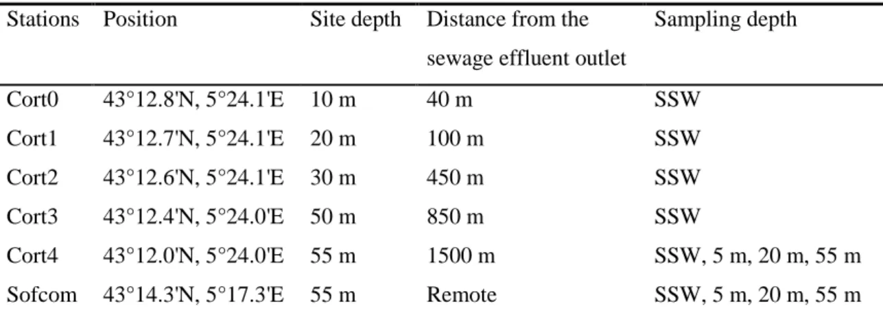
Table 1. Characteristics of the study sites, located in the Bay of Marseilles (northwestern Mediterranean Sea, France) and sampled from September 2008 to June 2010.
Stations Position Site depth Distance from the sewage effluent outlet
Sampling depth Cort0 43°12.8'N, 5°24.1'E 10 m 40 m SSW Cort1 43°12.7'N, 5°24.1'E 20 m 100 m SSW Cort2 43°12.6'N, 5°24.1'E 30 m 450 m SSW Cort3 43°12.4'N, 5°24.0'E 50 m 850 m SSW Cort4 43°12.0'N, 5°24.0'E 55 m 1500 m SSW, 5 m, 20 m, 55 m Sofcom 43°14.3'N, 5°17.3'E 55 m Remote SSW, 5 m, 20 m, 55 m Sampling dates: 23/09/08, 14/10/08, 14/11/08, 25/11/08, 19/02/09, 03/06/09, 23/06/09, 25/01/10, 08/04/10, 11/06/10, 16/06/10.
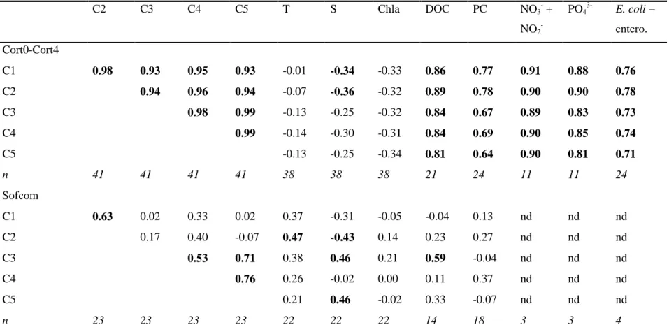
Table 2. Pearson’s correlation coefficients (r) of linear regressions between the fluorescence intensities of the five PARAFAC
components (C1-C5, in QSU) and the environmental parameters for the stations impacted (Cor0-Cort4) and not impacted (Sofcom) by the Marseilles sewage effluent.
C2 C3 C4 C5 T S Chla DOC PC NO3 + NO2 -PO4 3-E. coli + entero. Cort0-Cort4 C1 0.98 0.93 0.95 0.93 -0.01 -0.34 -0.33 0.86 0.77 0.91 0.88 0.76 C2 0.94 0.96 0.94 -0.07 -0.36 -0.32 0.89 0.78 0.90 0.90 0.78 C3 0.98 0.99 -0.13 -0.25 -0.32 0.84 0.67 0.89 0.83 0.73 C4 0.99 -0.14 -0.30 -0.31 0.84 0.69 0.90 0.85 0.74 C5 -0.13 -0.25 -0.34 0.81 0.64 0.90 0.81 0.71 n 41 41 41 41 38 38 38 21 24 11 11 24 Sofcom C1 0.63 0.02 0.33 0.02 0.37 -0.31 -0.05 -0.04 0.13 nd nd nd C2 0.17 0.40 -0.07 0.47 -0.43 0.14 0.23 0.27 nd nd nd C3 0.53 0.71 0.38 0.46 0.21 0.59 -0.04 nd nd nd C4 0.76 0.26 -0.02 0.00 0.11 0.37 nd nd nd C5 0.21 0.46 -0.02 0.33 -0.07 nd nd nd n 23 23 23 23 22 22 22 14 18 3 3 4
n: number of observations for each regression; nd: correlation coefficient not determined because of the too low number of observations. Correlation coefficients in bold are significant (p < 0.05).
Figure 1 43°12’N 43°18’N 05°12’E 05°24’E N 5 km 43°12’N 43°18’N 05°12’E 05°24’E N 5 km Mediterranean Sea Sofcom Frioul Islands Marseilles Cortiou Cove Treatment plant Huveaune River Raw SE P rado Cort4 Cort3 05°23’E Cort2 05°24’E 05°25’E 43°12’N 43°13’N N 0.5 km Cortiou Cove Marseilles SE :secondary treated SE + pretreated Huveaune waters Cort1 Cort0 France Pretreated Huveaune waters Secondary treated SE 43°12’N 43°18’N 05°12’E 05°24’E N 5 km 43°12’N 43°18’N 05°12’E 05°24’E N 5 km Mediterranean Sea Sofcom Frioul Islands Marseilles Cortiou Cove Treatment plant Huveaune River Raw SE P rado Cort4 Cort3 05°23’E Cort2 05°24’E 05°25’E 43°12’N 43°13’N N N 0.5 km Cortiou Cove Marseilles SE :secondary treated SE + pretreated Huveaune waters Cort1 Cort0 France Pretreated Huveaune waters Secondary treated SE
300 350 400 450 500 E m is s io n w a v e le n g th ( n m ) 0 0.1 0.2 0.3 0.4 0.5 0.6 0.7 L o a d in g 0 0.1 0.2 0.3 0.4 0.5 0.6 C4 C2 C3 250 300 350 400 450 500 Excitation wavelength (nm) 0 0.05 0.1 0.15 0.2 0.25 0.3 0.35 0.4 0 0.05 0.1 0.15 0.2 0.25 0.3 0.35 0.4 230 280 330 380 430 480 530 Wavelength (nm) 0 0.1 0.2 0.3 0.4 0.5 0.6 0.7 0.8 C1 λEx: < 230, 275 nm C5 λEm: 306 nm λEx: < 230, 270 nm λEm: 346 nm λEx: 280 nm λEm: 386 nm λEx: 235, 340 nm λEm: 310 nm λEx: 255, 365 nm λEm: 474 nm Tyrosine-like (peaks “B”) Tryptophan-like (peaks “T”) Marine humic-like (peak “M”) Humic-like (peaks “A” and “C”)
Humic-like (peaks “A” and “C”)
300 350 400 450 500 E m is s io n w a v e le n g th ( n m ) 0 0.1 0.2 0.3 0.4 0.5 0.6 0.7 L o a d in g 0 0.1 0.2 0.3 0.4 0.5 0.6 C4 C2 C3 250 300 350 400 450 500 Excitation wavelength (nm) 0 0.05 0.1 0.15 0.2 0.25 0.3 0.35 0.4 0 0.05 0.1 0.15 0.2 0.25 0.3 0.35 0.4 0 0.05 0.1 0.15 0.2 0.25 0.3 0.35 0.4 230 280 330 380 430 480 530 Wavelength (nm) 0 0.1 0.2 0.3 0.4 0.5 0.6 0.7 0.8 C1 λEx: < 230, 275 nm C5 λEm: 306 nm λEx: < 230, 270 nm λEm: 346 nm λEx: 280 nm λEm: 386 nm λEx: 235, 340 nm λEm: 310 nm λEx: 255, 365 nm λEm: 474 nm Tyrosine-like (peaks “B”) Tryptophan-like (peaks “T”) Marine humic-like (peak “M”) Humic-like (peaks “A” and “C”)
Humic-like (peaks “A” and “C”)
F ig u re 3 a ) T a 1 0 12 14 ° C16 18 20 22 C ort1 C ort2 C ort0 C ort3 C ort4 S ofcom a a a a a 3 7 .0 3 7 .2 3 7 .4 3 7 .6 3 7 .8 3 8 .0 3 8 .2 3 8 .4 b ) S C ort1 C ort2 C ort0 C ort3 C ort4 So fcom a ,b a ,b a a ,b a ,b b 0 1 2 3 4 5 6 C ort1 C ort2 C ort0 C ort3 C ort4 So fcom c ) C h la µg l-1 a a a a a a 0 50 1 0 0 1 5 0 2 0 0 2 5 0 C ort1 C ort2 C ort0 C ort3 C ort4 So fcom µM d ) D O C a a b b b b 0 40 80 1 2 0 1 6 0 2 0 0 2 4 0 C ort1 C ort2 C ort0 C ort3 C ort4 So fcom µM e ) P C a a b b b b 0 15 30 45 60 75 C ort1 C ort2 C ort0 C ort3 C ort4 S ofcom f) N O 3 -+ N O 2 -a a a b b b µM 0 1 2 3 4 5 6 C ort1 C ort2 C ort0 C ort3 C ort4 So fcom a a b b b b g ) P O 4 3 -0 20 40 60 80 1 0 0 1 2 0 C ort1 C ort2 C ort0 C ort3 C ort4 So fcom µM 103CFU 100 ml-1 a b b c c c h ) E . c o li + e n te ro c o c c i 1 0 0 a ) T a 1 0 12 14 ° C16 18 20 22 C ort1 C ort2 C ort0 C ort3 C ort4 S ofcom C ort1 C ort2 C ort0 C ort3 C ort4 S ofcom a a a a a 3 7 .0 3 7 .2 3 7 .4 3 7 .6 3 7 .8 3 8 .0 3 8 .2 3 8 .4 b ) S C ort1 C ort2 C ort0 C ort3 C ort4 So fcom C ort1 C ort2 C ort0 C ort3 C ort4 So fcom a ,b a ,b a a ,b a ,b b 0 1 2 3 4 5 6 C ort1 C ort2 C ort0 C ort3 C ort4 So fcom C ort1 C ort2 C ort0 C ort3 C ort4 So fcom c ) C h la µg l-1 a a a a a a 0 50 1 0 0 1 5 0 2 0 0 2 5 0 C ort1 C ort2 C ort0 C ort3 C ort4 So fcom C ort1 C ort2 C ort0 C ort3 C ort4 So fcom µM d ) D O C a a b b b b 0 40 80 1 2 0 1 6 0 2 0 0 2 4 0 C ort1 C ort2 C ort0 C ort3 C ort4 So fcom C ort1 C ort2 C ort0 C ort3 C ort4 So fcom µM e ) P C a a b b b b 0 15 30 45 60 75 C ort1 C ort2 C ort0 C ort3 C ort4 S ofcom C ort1 C ort2 C ort0 C ort3 C ort4 S ofcom f) N O 3 -+ N O 2 -a a a b b b µM 0 1 2 3 4 5 6 C ort1 C ort2 C ort0 C ort3 C ort4 So fcom C ort1 C ort2 C ort0 C ort3 C ort4 So fcom a a b b b b g ) P O 4 3 -0 20 40 60 80 1 0 0 1 2 0 C ort1 C ort2 C ort0 C ort3 C ort4 So fcom C ort1 C ort2 C ort0 C ort3 C ort4 So fcom µM 103CFU 100 ml-1 a b b c c c h ) E . c o li + e n te ro c o c c i 1 0 0
a c b c,d d a,b b a,b 0 20 40 60 80 100 120 140 160 180 Cor t1 Cor t2 Cor t0 Cor t3 Cor t4 Sof com Q S U
a) Total fluorescence
Cor t1 Cor t2 Cor t0 Cor t3 Cor t4 Sof com 0 10 20 30 40 50 60 a a a a a ae) C4, humic-like
% 0 10 20 30 40 50 60 Cor t1 Cor t2 Cor t0 Cor t3 Cor t4 Sof comc) C2, tryptophan-like
a a a a,b % a a,b b 0 10 20 30 40 50 60 a a a Cor t1 Cor t2 Cor t0 Cor t3 Cor t4 Sof comf) C5, humic-like
% 0 10 20 30 40 50 60 Cor t1 Cor t2 Cor t0 Cor t3 Cor t4 Sof com a a a a a,b b %d) C3, marine humic-like
Cor t1 Cor t2 Cor t0 Cor t3 Cor t4 Sof comb) C1, tyrosine-like
0 5 10 15 20 25 30 35 a a b a,b a,b a,b % a c b c,d d a,b b a,b 0 20 40 60 80 100 120 140 160 180 Cor t1 Cor t2 Cor t0 Cor t3 Cor t4 Sof com Cor t1 Cor t2 Cor t0 Cor t3 Cor t4 Sof com Q S Ua) Total fluorescence
Cor t1 Cor t2 Cor t0 Cor t3 Cor t4 Sof com Cor t1 Cor t2 Cor t0 Cor t3 Cor t4 Sof com 0 10 20 30 40 50 60 a a a a a ae) C4, humic-like
% 0 10 20 30 40 50 60 Cor t1 Cor t2 Cor t0 Cor t3 Cor t4 Sof com Cor t1 Cor t2 Cor t0 Cor t3 Cor t4 Sof comc) C2, tryptophan-like
a a a a,b % a a,b b 0 10 20 30 40 50 60 a a a Cor t1 Cor t2 Cor t0 Cor t3 Cor t4 Sof com Cor t1 Cor t2 Cor t0 Cor t3 Cor t4 Sof comf) C5, humic-like
% 0 10 20 30 40 50 60 Cor t1 Cor t2 Cor t0 Cor t3 Cor t4 Sof com Cor t1 Cor t2 Cor t0 Cor t3 Cor t4 Sof com a a a a a,b b %d) C3, marine humic-like
Cor t1 Cor t2 Cor t0 Cor t3 Cor t4 Sof com Cor t1 Cor t2 Cor t0 Cor t3 Cor t4 Sof comb) C1, tyrosine-like
0 5 10 15 20 25 30 35 a a b a,b a,b a,b %a b 0 20 40 60 80 100 120 140 160 a) Total fluorescence a b Q S U Cor t0-S Cor t0-W Sofc om-S Sofc om-W -S: spring + summer -W: autumn + winter 0 10 20 30 40 50 60 Cor t0-S Cor t0-W Sofc om-S Sofc om-W a a a a e) C4, humic-like % % 0 10 20 30 40 50 60 70 Cor t0-S Cor t0-W Sofc om-S Sofc om-W c) C2, tryptophan-like a a a b 0 10 20 30 40 50 60 70 f) C5, humic-like % a a a b Cor t0-S Cor t0-W Sofc om-S Sofc om-W 0 10 20 30 40 50 60 % d) C3, marine humic-like a b a a Cor t0-S Cor t0-W Sofc om-S Sofc om-W 0 10 20 30 40 50 60 70 b) C1, tyrosine-like % a a a b Cor t0-S Cor t0-W Sofc om-S Sofc om-W