HAL Id: lirmm-01275509
https://hal-lirmm.ccsd.cnrs.fr/lirmm-01275509
Submitted on 17 Feb 2016
HAL is a multi-disciplinary open access
archive for the deposit and dissemination of
sci-entific research documents, whether they are
pub-lished or not. The documents may come from
teaching and research institutions in France or
abroad, or from public or private research centers.
L’archive ouverte pluridisciplinaire HAL, est
destinée au dépôt et à la diffusion de documents
scientifiques de niveau recherche, publiés ou non,
émanant des établissements d’enseignement et de
recherche français ou étrangers, des laboratoires
publics ou privés.
Characterization of Outliers in Categorical Data
Dino Ienco, Ruggero Pensa, Rosa Meo
To cite this version:
Dino Ienco, Ruggero Pensa, Rosa Meo. A Semi-Supervised Approach to the Detection and
Char-acterization of Outliers in Categorical Data. IEEE Transactions on Neural Networks and Learning
Systems, IEEE, 2017, 28 (5), pp.1017-1029. �10.1109/TNNLS.2016.2526063�. �lirmm-01275509�
A Semi-Supervised Approach to the Detection and
Characterization of Outliers in Categorical Data
Dino Ienco, Ruggero G. Pensa, and Rosa Meo
Abstract—In this paper we introduce a new approach of semi-supervised anomaly detection that deals with categorical data. Given a training set of instances (all belonging to the normal class), we analyze the relationships among features for the extraction of a discriminative characterization of the anomalous instances. Our key idea is to build a model characterizing the features of the normal instances and then use a set of distance-based techniques for the discrimination between the normal and the anomalous instances. We compare our approach with the state-of-the-art methods for semi-supervised anomaly detection. We empirically show that a specifically designed technique for the management of the categorical data outperforms the general-purpose approaches. We also show that, in contrast with other approaches that are opaque because their decision cannot be easily understood, our proposal produces a discriminative model that can be easily interpreted and used for the exploration of the data.
Index Terms—Anomaly detection, distance learning, categori-cal data, semi-supervised learning.
I. INTRODUCTION
I
N many application domains, such as fraud detection,intru-sion detection, satellite image analysis and fault diagnosis, the identification of instances that diverge from the expected behavior is a crucial task. The detection of these instances (called anomalies or outliers) has multiple applications: it can be used to spot possible noisy data and clean it, thus enhancing the analysis, or to identify undesirable events when they happen.
From a data analysis point of view, outlier/anomaly detec-tion is the problem of finding abnormal instances in the data, where data are considered normal if they fit some expected distribution. It is a multi-disciplinary research area that has been investigated extensively by researchers from statistics, data mining and machine learning. In practice, it can be defined as a classification task where the goal is to decide whether an incoming instance is normal or anomalous. For a comprehensive survey of this area we refer to [1].
Though the goal is well defined, there exist multiple anomaly detection techniques that can be classified on the basis of two main perspectives: (1) the availability of sup-plementary information on training data (e.g., class labels), and (2) the type of data they manipulate.
Concerning the first point of view, in the literature we identify three classes of approaches: supervised, unsupervised
D. Ienco is with IRSTEA, UMR TETIS, F-34093 Montpellier, France and with LIRMM, F-34090 Montpellier, France (e-mail: dino.ienco@irstea.fr)
R.G. Pensa and R. Meo are with the Department of Computer Science, University of Torino I-10149 Torino, Italy (e-mail: ruggero.pensa@unito.it, rosa.meo@unito.it)
and semi-supervised [1]. Supervised techniques are often handled using classical machine learning techniques where the problem is treated as a binary classification problem with the abnormal class being poorly represented (imbalanced data) [2]. Unsupervised techniques detect anomalies without knowledge on the class variable [3]. They assume that anomalies are geometrically separated in the features space from the normal instances. These techniques usually employ clustering algo-rithms assuming that normal instances are closer to each others than to outliers which are placed in low density regions. Hence, they require the availability at processing times of instances from all the classes.
Unsupervised and supervised anomaly detection techniques represent the majority of the research work in the area of anomaly/outlier detection. A limitation of these approaches consists in the fact that they assume that training data contain both normal and abnormal instances. In many applications this is a strong requirement, since abnormal data are often difficult or expensive to obtain. For instance, in aircraft engine fault detection, collecting data related to damaged components requires those components to be sabotaged which is costly and extremely difficult.
A solution to this point comes from the semi-supervised approaches [1], [4] that do not require anomalous instances in the training phase: they build a model of the normal class in the training data and recognize the anomalies in test data as those instances that most differ from the normal model. As a positive side-effect, when normality shifts it may re-learn the data model.
Concerning the second point of view, most anomaly de-tection methods apply to numerical or ordinal attributes for which the normality can be defined by a proximity notion between instances described as vectors in a m-dimensional space. When objects are described by numerical features, there is a wide range of possible proximity measures.
Actually data are often described by categorical attributes that take values in a set of unordered nominal values, and can-not be mapped into ordinal values without loss of information. For instance the mapping of a marital status attribute value (married or single) or a person’s profession (engineer, teacher, etc.) to a numerical value is not straightforward. This makes it impossible even to rank or compute differences between two values of the feature vectors. For categorical data the simplest comparison measures are derived from overlap [5] in which the proximity between two multivariate categorical entities is proportional to the number of attributes in which they match. Clearly, these distance metrics do not distinguish between the different values which is a strong limitation since
it prevents to capture similarities that are clearly identified by human experts.
In this paper we propose a solution to the problem of anomaly detection in categorical data with a semi-supervised setting. Our approach is based on DILCA, a distance learning framework we introduced in [6]. The key intuition of DILCA is that the distance between two values of a categorical
attribute Ai can be determined by the way in which they
co-occur with the values of other attributes in the dataset : if two
values of Ai are similarly distributed w.r.t. other attributes
Aj (with i 6= j), the distance is low. The added value of
this proximity definition is that it takes into consideration the context of the categorical attribute, defined as the set of the other attributes that are relevant and non redundant for the determination of the categorical values. Relevancy and redundancy are determined by the symmetric uncertainty measure that is shown to be a good estimate of the correlation between attributes [7].
We validate our method by an extensive experimental anal-ysis showing that our new approach based on data proximity outperforms the state-of-the-art semi-supervised methods in the field of anomaly detection considering categorical data. This also empirically demonstrates that simply adapting an existing numerical approach to categorical data is not a suf-ficient strategy to successfully detect anomalies. Categorical data needs ad-hoc strategies. Moreover, the experiments show that our method is competitive to other methods that directly consider categorical data. A recent proposal like FRaC [8] that directly handles categorical data is based on predictive models: as a consequence its accuracy performance heavily depends on the predictor models and on the tuning of many parameters. Moreover, the choice of the predictor models can be done only by the experts. Our method, instead, is based on the proximity notion which is intuitive for the end-user. Last but not least, a positive side-effect of our method, is that the proximity values between instances provide a descriptive model that can be easily visualized and allows the exploration and organization of the domain knowledge by the analyst. The key contributions of our work are the following:
• We design an anomaly detection framework for
cate-gorical data based on the distance learning approach presented in [6];
• We embed the distance learning algorithm within
differ-ent ranking strategies and show that our approach returns good outlier candidates for each of the four proposed ranking strategies;
• We compare our method with state-of-the-art
semi-supervised outlier detection methods. This comparison highlights the necessity of designing the anomaly detec-tion specifically for categorical data.
• We show that our method is not simply a working
method, but it provides also explanatory insights about the data.
The remainder of this paper is organized as follows: Section II discusses related work. In section III we briefly explain the DILCA framework for learning distances from categorical data [6]. The distance based algorithms, the complexity
discus-sions and the exploration capabilities are presented in Section IV. In Section V we report the experiments while section VI concludes.
II. RELATED WORK
Outlier, or anomaly detection, has always attracted a lot of research interest since its first definition in the late Sixties [9]. With the advent of data mining and the advances in machine learning that occurred in the 1990s, the research on anomaly detection gained new impetus and gave rise to many novel approaches and algorithms [1]. Even though all these approaches can be classified depending on various aspects, here we present some relevant recent algorithms by underlying the type of data they handle and how they use data labels when available. In particular, as regards the latter aspect, anomaly detection approaches can be grouped into three classes: un-supervised methods, which ignore whether training instances are normal or anomalous; supervised methods, which leverage both normal/anomalous class labels; semi-supervised methods, which handle data that exhibit a partial labeling (generally, only normal instances are known). Here, we will not address supervised anomaly detection since the problem is similar to building predictive models in the presence of imbalanced or skewed class distributions [2].
Unsupervised and semi-supervised anomaly detection A well-known proposal of unsupervised outlier detection is LOF [10] that employs the distance between objects to detecting local outliers that differ from dense regions. The distance is computed on the k nearest neighbors: hence, LOF strongly depends on the setting of the parameter k. In [11] a cluster-based technique is employed with a kernel-based technique for a robust segmentation of the customers base and outlier identification. In [12], the authors introduce an angle-based outlier method that employs the divergence in the objects directions. [3] is also focused on unsupervised anomaly detection on numerical data and categorical attributes are often ignored, although it is well-known that a misused or unadapted distance measure may negatively affect the results [13].
Semi-supervised anomaly detection has attracted more re-search interests in the last fifteen years. A first formulation was given in [14] with a semi-supervised outlier detection algorithm based on SVM. The so-called One-Class SVM algorithm maps input data into a high dimensional feature space and iteratively finds the maximal margin hyperplane which best separates the training data from the origin. In [15] a statistical outlier detection framework is introduced: uLSIF. It assumes that the density ratio between training and test set tends to be small for candidate outliers and it estimates a weight (importance factor) for each training instance. Both these methods are studied principally for numerical or ordinal data [16]. Another semi-supervised method is FRaC [8], which uses normal instances to build an ensemble of feature classifi-cation models, and then identifies instances that disagree with those models as anomalous. It is not specifically tailored on categorical data but it can adopt any classification algorithms that work well on each specific feature type. All these semi-supervised methods are compared with ours in Section V.
Anomaly detection in categorical domains
Many of the early (unsupervised) methods to mine outliers in categorical domains are based on frequent itemset min-ing such as [17] and [18]. More recently, the problem of mining outliers in the categorical domain has been tackled by directly processing the data. In [19] a greedy algorithm is presented and adopts a principle based on entropy-change after instances removal. [20] proposes a method that assigns a score to each attribute-value pair based on its frequency. Objects with infrequent attribute values are candidate outliers. Both these approaches are unsupervised. In [21] the authors propose an unsupervised method for detecting anomalous patterns in categorical datasets which is a slightly different task than the detection of anomalous instances. [22], instead, is a recent unsupervised method for categorical data that marks as anomalies those instances whose compression cost is higher than the cost required by the norm in a pattern-based compression mechanism based on the Minimum Description Length principle. The norm is defined as the patterns that compress the data well (with a low compression cost). [23] is also a pattern-based compression method, but, contrary to [22], it works in a semi-supervised setting. However, its detection accuracy is, on average, worse than the accuracy of OSVM [14]. Yet it requires the computation of a collection of frequent itemsets and a minimal support threshold to mine these.
Our work is motivated by the necessity of having a specific semi-supervised technique that directly manages categorical data. Our solution embeds a distance learning technique for categorical data [6] into a distance based algorithm which serves to characterize the normal class. This characterization is successively employed to detect the anomalous instances in a semi-supervised scenario. Our particular choice also enables a human understandable characterization aiming at supporting the analyst’s work. Investigating suitable measures for computing distances between categorical data instances is also an active field. In this context, another relevant contribu-tion is [24] in which the authors evaluate the performance of different distance measures for categorical data for the anomaly detection task which is known to be affected in a marked way by the employed measure. To this purpose, the unsupervised algorithm LOF is combined with 14 different distance measures. In this work, we don’t use this latter solution since, as we demonstrated empirically in [6], our distance learning approach outperforms the most efficient metrics presented in [24].
III. DISTANCE LEARNING FOR CATEGORICAL ATTRIBUTES
A brief summary of DILCA (DIstance Learning for Cat-egorical Attributes) is provided here. This is a framework for computing distances between any pair of values of a categorical attribute. DILCA was introduced by Ienco et al. in [6] but was limited to a clustering scenario.
To illustrate this framework, we consider the dataset de-scribed in Figure 1(a), representing a set of sales dede-scribed by means of five categorical attributes: Age, whose possible values from the set {young, adult, senior} describe the client’s
age; Gender, which describes the client’s gender by means of the values {M, F }; Profession, whose possible values are {student, unemployed, businessman, retired}, Product whose domain is {mobile, smartphone, tablet} and finally
Sales department whose domain values {center, suburbia}
give the location area of the store in which the sales occurred. The contingency tables in Figure 1(b) and Figure 1(c) show how the values of attribute Product are distributed w.r.t. the two attributes Profession and Sales department. From Figure 1(c), we observe that Product=tablet occurs only with
Sales dep=centerand Product=mobile occurs only with Sales
dep=suburbia. Conversely, Product=smartphone is satisfied both when Sales dep=center and Sales dep=suburbia. From this distribution of data we infer that, in this particular context,
tablet is more similar to smartphone than to mobile because
the probability of observing a sale in the same department is closer. However, if we take into account the co-occurrences of Product values and Profession values (Figure 1(b)) we may notice that Product=mobile and Product=tablet are closer to each-other rather than to Product=smartphone, since they are bought by the same professional categories of customers at a similar extent.
This example shows that the distribution of the values in the contingency table may help to define a distance between the values of a categorical attribute, but also that the context matters. Let us now consider the set F = {X1, X2, . . . , Xm} of m categorical attributes and dataset D in which the in-stances are defined over F . We denote by Y ∈ F the target attribute, which is a specific attribute in F that is the target of the method, i.e., the attribute on whose values we compute the distances. DILCA allows to compute a context-based distance between any pair of values (yi, yj) of the target attribute Y on the basis of the similarity between the probability distributions of yiand yj given the context attributes, called C(Y ) ⊆ F \Y .
For each context attribute Xi ∈ C(Y ) DILCA computes the
conditional probability for both the values yi and yj given the
values xk ∈ Xi and then it applies the Euclidean distance.
The Euclidean distance is normalized by the total number of considered values: d(yi, yj) = s P X∈C(Y ) P xk∈X(P (yi|xk) − P (yj|xk)) 2 P X∈C(Y )|X| (1) The selection of a good context is not trivial, particularly when data is high-dimensional. In order to select a relevant and non redundant set of features w.r.t. a target one, we adopt the FCBF method: a feature-selection approach originally presented by Yu and Liu [7] exploited in [6] as well. The
FCBFalgorithm has been shown to perform better than other
approaches and its parameter-free nature avoids the tuning step generally needed by other similar approaches. It takes into account the relevance and the redundancy criteria between attributes. The correlation for both criteria is evaluated through the Symmetric Uncertainty measure (SU). SU is a normalized version of the Information Gain [25] and it ranges between 0 and 1. Given two variables X and Y , SU=1 indicates that the knowledge of the value of either Y or X completely predicts the value of the other variable; 0 indicates that Y
ID Age Gender Profession Product Sale dep.
1 young M student mobile suburbia
2 senior F retired mobile suburbia
3 senior M retired mobile suburbia
4 young M student smartphone suburbia
5 senior F businessman smartphone center
6 adult M unemployed smartphone suburbia
7 adult F businessman tablet center
8 young M student tablet center
9 senior F retired tablet center
10 senior M retired tablet center
(a) Sales table
mobile smartphone tablet
student 1 1 1
unemployed 0 1 0
businessman 0 1 1
retired 2 0 2
(b) Product-Profession
mobile smartphone tablet
center 0 1 4
suburbia 3 2 0
(c) Product-Sales dep.
Fig. 1. Sales: a sample dataset with categorical attributes (a) and two related contingency tables (b and c).
and X are independent. During the step of context selection, a set of context attributes C(Y ) for a given target attribute
Y is selected. Informally, these attributes Xi ∈ C(Y ) should
have a high value of the Symmetric Uncertainty and are
not redundant. SUY(Xi) denotes the Symmetric Uncertainty
between Xi and the target Y . DILCA first produces a ranking
of the attribute Xi in descending order w.r.t. SUY(Xi). This
operation implements the relevance step. Starting from the
ranking, it compares each pairs of ranked attributes Xi and
Xj. One of them is considered redundant if the Symmetrical
Uncertainty between them is higher than the Symmetrical Uncertainty that relates each of them to the target. In particular,
Xj is removed if Xi is in higher position of the ranking and
the SU that relates them is higher than the SU that relates
each of them to the target (SUXj(Xi) > SUY(Xi) and
SUXj(Xi) > SUY(Xj)). This second part of the approach
implements the redundancy step. The results of the whole procedure is the set of attributes that compose the context C(Y ).
At the end of the process, DILCA returns a distance model
M = {MXi| i = 1, . . . , m}, where each MXi is the matrix
containing the distances between any pair of values of attribute
Xi, computed using Eq. 1.
IV. SEMI-SUPERVISED ANOMALY DETECTION FOR
CATEGORICAL DATA
The distance learning approach described in the previous section has been successfully employed in a clustering sce-nario (see [6] for details). In this section, we define a semi-supervised anomaly detection framework for categorical data which takes benefit of DILCA.
Before entering the core of our approach of anomaly de-tection for categorical datasets, we recall the definition of a semi-supervised anomaly detection problem [1].
Let D = {d1, . . . , dn} be a set of n normal data objects
described by a set of categorical features F . Let T =
{t1, . . . , tm} be another set of m data objects described by the same set F , and such that part of the objects are normal
and the remaining ones are abnormal. To distinguish between normal and abnormal objects, we define a class variable class which takes values in the set {A, N }, and such that ∀d ∈ D, class(d) = N and ∀t ∈ T, class(t) ∈ {A, N }. The goal of the semi-supervised anomaly detection framework is to decide whether a previously unseen data object t ∈ T is normal or abnormal, by learning the normal data model from D.
Typically in anomaly detection there are two ways to present the results: the first one is to assign a normal/abnormal label to each test data instance; the second is to give an anomaly score (a sort of anomaly degree) to each tested instance. The last method is often preferred since it enables the user to decide a cutoff threshold over the anomaly score, or to retain the top-k instances rantop-ked by the anomaly score values. Depending on the constraints w.r.t. the admitted false positives or true negatives present in the results, the user may set a high or low threshold, or decide to consider a high or low value of k. Our approach supplies the second type of output: given a training data set D, the normality model learned on D and a test instance t ∈ T , it returns the value of the anomaly score of t.
Our approach, called SAnDCat (Semi-supervised Anomaly Detection for Categorical Data), consists of two phases: during the first phase, we learn a model of the normal class N from the training data D; in the second phase we select k representative objects from D and we take them as a reference for the computation of the anomaly score of each test instance. In details, SAnDCat works as follows:
1) It learns a model consisting of a set of matrices M =
{MXi}, one for each attribute Xi ∈ F . Each element
mi(j, l) = d(xij, xil) is the distance between the values xi
j and xil of the attribute Xi, computed using DILCA
by evaluation of Equation 1 over the training dataset D. These matrices provide a summarization in terms of the DILCA distance function on the distribution of the
values of the attributes Xi given the other attributes in
the instances of the normal class.
to compute a distance between any two data instances
d1 and d2 on the basis of the DILCA distance between
the categorical values, using the following formula: dist(d1, d2) = s X MXi∈M mi(d 1[Xi], d2[Xi])2 (2)
where d1[Xi] and d2[Xi] are respectively the values
of the attribute Xi in the objects d1 and d2. Finally,
SAnDCat measures the outlier score OS associated to
each test instance t ∈ T as the sum of the distances between t and a subset of k (1 ≤ p ≤ k ≤ n) instances
dp belonging to D, i.e.: OS(t) = k X p=1 dist(t, dp) (3)
where dist(t, dp) is computed using Equation 2.
The key intuition behind SAnDCat is that a distance that fits for the training dataset D should fit also for the instances
tn ∈ T whose class(tn) = N , but not for the instances ta
whose class(ta) = A. Hence, we expect that those instances
of T belonging to the normal class N are closer to instances in D than those belonging to the abnormal class A. The reason is that combinations of characteristic attribute values of the normal instances in D produce low distance values between the normal instances, and these ones are maintained also in the normal instances of the test set T . On the contrary these characteristic attribute values are not necessarily present in the abnormal instances and this produces higher values of the distances between a normal and an abnormal instance.
A. Selecting k data representatives
We discuss now the problem of the selection of a represen-tative set of k instances of D for the computation of the outlier score. Here, we present four different heuristics: two of them depend on the position of the test instance in the feature space, and require then to be re-executed for each test instance; the other two are executed once for all, since they do not depend on the tested instance. For this reason, the last two heuristics are suitable also for on-line outlier detection, in application where data need to be analyzed in real time. In the following, we present in detail each heuristic strategy.
• Minimum Distance Top-k (MinDTK): given a test
instance t, we compute the outlier score considering the k training instances that are closer to t. This operation requires n distance computations to compute distances. The complexity of choosing the top k similar instances for each test instance is then O(n). To process the whole test set T , this strategy requires O(mn) operations. Supposing m ∼ n, the overall complexity of this heuristic is O(n2).
• Maximum Distance Top-k (MaxDTK): this strategy is
similar to the previous one, except that in this case we select the k instances that are most distant from t. The complexity is the same as in the previous method.
• Random k (RandK): we select k random instances from
the training set, and we compute the outlier score using
these instances for all the test set. This strategy requires O(k × m) operations. Supposing k m and m ∼ n, the overall complexity is O(n). This method is the less expensive from the computational point of view.
• Central k (CentralK): this heuristic selects the k most
central instances in the training set. As regards the
cen-trality of an instance di ∈ D, we propose the following
measure that should be minimized to find the k most central instances:
CD(di) =
X
dp∈D, dp6=di
dist(di, dp)2
We use these k instances for computing the outlier score
of the whole test set. This strategy requires O(n2)
opera-tions to compute centrality values, O(n log n) operaopera-tions to rank the training instances and O(k × m) operations to compute the outlier score of the test set. Supposing k m and m ∼ n, the overall complexity of this
heuristic depends on the first step, i.e., O(n2). However,
once the central instances have been selected, it only requires k distance computations to process each test instance.
B. Overall complexity
The overall complexity of SAnDCat depends on three factors: (1) the complexity of the training algorithm, which depends on DILCA, (2) the selected strategy for computing the k data representatives, and (3) the type of output (threshold-based or ranked list). Concerning (1), from [6] it turns out that
the complexity of DILCA is O(nl2log l), where l = |F |. For
(2), the worst case is given by the first two strategies, which
require O(n2) operations. Finally, for (3), using a threshold
requires constant time, while ranking the test instances requires O(m log m) operations. Supposing m ∼ n, in the worst
case, SAnDCat requires O(nl2log l + n2+ n log n) operations.
In general l n of at least one order of magnitude:
we can assume then that the component O(n2) prevails on
O(nl2log l), and the overall complexity is O(n2) (we show
this empirically in Section IV-B). When using the RandK strategy, the second component is O(n), leading to an overall
complexity of O(nl2log l).
C. Characterization, inspection and exploration of anomalies In addition to the anomaly detection abilities (discussed in Section V) our approach also supports the characteri-zation and the exploratory analysis of the anomalies. To this purpose it provides the analyst with the explana-tory proximity values between the values of the cate-gorical attributes. In order to concretely show the added value of our distance learning approach, we analyze in detail the Contact-Lenses dataset [26]. The dataset con-tains 24 instances belonging to 3 classes: soft, hard, none.
Each instance is described by four attributes: Age ∈
{young, pre-presbyotic, presbyotic}, Spectacle prescrip ∈
{myope, hypermetrope}, Astigmatism ∈ {no, yes},
T ear prod rate ∈ {re− duced, normal}. Its small size allows us to show the behavior of our approach and to easily
Age young pre-presbyotic presbyotic
young 0 0.2357 0.4714
pre-presbyotic 0.2357 0 0.2357
presbyotic 0.4714 0.2357 0
(a)
Tear Prod Rate normal reduced
normal 0 0.6680 reduced 0.6680 0 (b) Astigmatism yes no yes 0 0.2202 no 0.2202 0 (c)
Spectacle Prescrip myope hypermetrope
myope 0 0.2202
hypermetrope 0.2202 0
(d)
Fig. 2. Distance matrices for attribute Age (a), Tear prod rate (b),
Astigma-tism(c) and Spectacle prescrip (d) in the instances of the normal class
give a rational explication of the obtained results. In order to be used for the purpose of anomaly detection, we update the dataset to be organized in two classes: the normal class including all the instances from the original class (none) and the abnormal class including all the instances for which one of the contact lenses types was prescribed (hard or soft). Then for training, we apply DILCA to learn the distance matrices using the instances alternatively from one of the two resulting classes (normal and abnormal). In Table I for each feature we show the attributes belonging to the related context. For instance we observe that attribute Astigmatism is always correlated with (Spectacle prescrip, Tear prod rate). This is actually confirmed by a common knowledge on ophthalmology: astig-matism is often related to a high production of tears. Also, we observe that tear production is related to age, as expected. When we consider the abnormal class, attribute Age becomes part of the context of all the attributes. This also confirms a medical common-sense, since age is an influencing factor in eyesight problems.
In Figure 2 and Figure 3 we report the four distance matrices learned by DILCA in the normal and abnormal cases. Let us first consider the normal case (Figure 2). We observe that a difference between the values of the attribute Tear prod rate has more influence on the final distance (because the contribu-tion to the distance is higher) than a mismatch on the attribute
Ageor on Astigmatism. As regards the attribute Age we notice
that the mismatch between young and presbyotic has more impact then all the other possible mismatches on the values of Age. This distance matrix is valid even considering the order that exists among the three values according to their real meaning: young, pre-presbyotic and presbyotic. When we look at the abnormal class (Figure 3) the distance matrices for
Astigmatism and Spectacle prescip are confirmed, while the
differences between the values of Tear prod rate appear more significant (they influence at a greater extent the distances between the instances of this class). The contribution to the distances between the values of the attribute Age, instead,
Age young pre-presbyotic presbyotic
young 0 0.1368 0.1949
pre-presbyotic 0.1368 0 0.1144
presbyotic 0.1949 0.1144 0
(a)
Tear Prod Rate normal reduced
normal 0 1.0 reduced 1.0 0 (b) Astigmatism yes no yes 0 0.2430 no 0.2430 0 (c)
Spectacle Prescrip myope hypermetrope
myope 0 0.2430
hypermetrope 0.2430 0
(d)
Fig. 3. Distance matrices for attribute Age (a), Tear prod rate (b),
Astigma-tism(c) and Spectacle prescrip (d) in the instances of the abnormal class
looks less significant. Indeed, Age is part of the context of the other attributes for this class (it contributes already to the distance computation of all the other attributes) but in isolation it does not help much to detect instances of this class.
1) The Attribute Model Impact: Obviously, looking at each
distance matrix individually can be frustrating, especially when dealing with high-dimensional data. We then provide an automated way to measure the impact of each attribute in the distance model and visualize the contribution of all attributes at a glance. We recall that the model generated by SAnDCat
supplies a set of matrices M = {MXi| i = 1, . . . , m} (one
for each attribute Xi). Each of them corresponds to a
point-wise distance matrix representing the distance between each
pair of values of a given attribute Xi. The attribute model
impactof Xi, namely I(Xi), is computed as the mean of the
upper (or lower) triangular part of the corresponding matrix
MXi = {m i (k, l)}: I(Xi) = PN −1 k=1 PN l=k+1m i(k, l) N (N − 1)/2
where N is the number of values taken by the attribute Xi.
Clearly, the attribute impact takes values in the interval [0, 1]
and higher values of I(Xi) indicate a stronger impact of the
attribute on the distance. The attribute model impact computed for the normal and abnormal classes of Contact-Lenses are given in Table II. It is clear that the attribute Age helps to detect well the instances of the normal class (even better for the normal class is the attribute Tear Prod Rate); although
Ageresults quite insignificant in detecting the instances of the
abnormal class, while the other three attributes work better.
2) The Attribute Distance Impact: Since our method does
not compute any distance model for the abnormal class (but only for the normal class), the attribute model impact can only be employed when a sufficient number of anomalous instances has been detected. However, a similar principle can be applied to any individual test instance. In this case, instead of computing the attribute model impact, we measure the contribution of each attribute on the distance between the test
TABLE I
CONTACT-LENSESATTRIBUTECONTEXTS FOR NORMAL AND ABNORMAL CLASSES
Context Attributes
Attribute Normal class Abnormal class
Age Tear prod rate Spectacle prescrip, Tear prod rate
Spectacle prescrip Astigmatism, Tear prod rate Age, Astigmatism, Tear prod rate
Astigmatism Spectacle prescrip, Tear prod rate Age, Spectacle prescrip, Tear prod rate
Tear prod rate Age, Spectacle prescrip Age
TABLE II
THE ATTRIBUTE MODEL IMPACT AND DISTANCE IMPACT FOR THE ATTRIBUTES OFContact-Lenses.
Attribute model impact
Class Age Tear Prod Rate Astigm. Spectacle P.
normal 0.3143 0.6680 0.2202 0.2202
abnormal 0.1487 1.000 0.2430 0.2430
Attribute distance impact
Class Age Tear Prod Rate Astigm. Spectacle P.
abnormal 0.2165 0.5344 0.1109 0.1109
instance and the instances from the normal class. For a given
attribute Xi, an anomalous instance ta and the set of normal
instances D, the attribute distance impact of Xiin ta, namely
I(Xi, ta) is given by:
I(Xi, ta) = P dj∈Repr(D)m i(t a[Xi], dj[Xi]) |Repr(D)|
where ta[Xi] and dj[Xi] are respectively the values of the attribute Xiin the instances ta and dj and mi(ta[Xi], dj[Xi])
is the corresponding element in MXi ∈ M. Notice that the
set of instances dj∈ D considered for the computation of the
attribute distance impact is the set Repr(D), i.e., the set of the representative instances of the normal class D selected by any of the methods described in Section IV-A.
The attribute distance impact takes values in the interval
[0, 1]: a higher value of I(Xi) indicates a stronger impact of
the attribute on the distance between the abnormal instance and the normal ones. The average of the values of the attribute distance impact for each attribute, where the average is computed for all the anomalous instances of Contact-Lenses is given in Table II.
The expressiveness of the attribute distance impact can be further exploited by means of some visual analytic tool. For instance, in Figure 4 we employ the well known word cloud paradigm. A word cloud is a visual representation for text data where the importance of each word is shown with the font size and/or its color. In our application, the font size of each attribute is proportional to its impact. The two clouds in Figure 4(a) and 4(b) clearly show the impact change of the attribute Age when moving from the instances of the normal class to the instances of the abnormal one. Figure 4(c), instead, shows the higher impact of some attributes (in particular of Tear Prod Rate) in terms of the attribute distance impact for the computation of the distance between abnormal instances and the instances of the normal class.
tearprodrate
age spectacleprescrip astigmatism (a)tearprodrate
age spectacleprescrip astigmatism (b)tearprodrate
age spectacleprescrip astigmatism (c)Fig. 4. Word clouds for the attribute model impact in Contact-Lenses for the instances of the normal class (a), the abnormal one (b) and the cloud for the attribute distance impact for the instances of the abnormal class (c).
D. Exploration of the data by theDILCA distances
Finally, our method also supports visual analytic tools for the exploration of the data and the visualization of the anomalous instances. In fact, differently from the competitors,
SAnDCatcomputes a distance model (provided by the DILCA
distances) that can be employed to visualize and explore anomalies using the Multi Dimensional Scaling algorithm [27]. This well-known technique is usually employed to derive an m-dimensional representation of a given set of instances (points) by only computing all the point-to-point distances. It computes a geometrical projection of the data points such that the original distances are preserved as much as possible. The only required parameter is the number of dimensions m. Figure 5 shows the multi-dimensional scaling representation of 9 test instances from Contact-lenses plotted in a 2-dimensional space (m = 2). The point-to-point distance has been computed by equation 2 having selected only k = 15 representative
training instances dj. Notice that the projection of some
of the instances in the 2-dimensional space makes some of the instances coincide in the same point. The picture shows quite a sharp separation between the normal instances and the abnormal ones (the instances from the opposite classes coincide only in two points out of six). This confirms that the instances coming from the opposite classes tend to have different attribute values and are placed in a different region of the space. Moreover, the distances between instances of the opposite classes are on average higher than the distances between instances of the same class.
V. EXPERIMENTS
To assess the quality of our approach we conducted several experiments on real world categorical datasets. In this section we first evaluate the four heuristics, for different values of k. Then, we compare our approach with state-of-the-art methods. Finally, we present a simple example to analyze the obtained
-0.4 -0.2 0 0.2 0.4 -0.4 -0.2 0 0.2 0.4 2nd coordinate 1st coordinate Normal Points Abnormal Points
Fig. 5. Test instances visualized using Multi Dimensional Scaling for Contact-Lenses.
model and illustrate how this model could be used to improve the exploratory analysis.
To evaluate the performance of an outlier detection al-gorithm, we must take into account both the detection rate (the amount of instances of the abnormal class found by the algorithm) and the detection error (the amount of instances of the normal class that the algorithm misjudges as outliers). To consider both measures at the same time, it is common to evaluate the results using the Area Under the Curve (AUC) [28]. In this work, we use the approach proposed in [29], in which the AUC score is computed with a closed-form formula:
AU C =S0− n0(n0+ 1)/2
n0n1
where n0 is the number of test instances belonging to the
normal class, n1is the number of abnormal test instances and
S0=P
n0
i=1ri, where ri is the rank given by the class model
of the normal class to the i-th normal instance in the test set. In our case it is the OS score given to each normal instance in the test set.
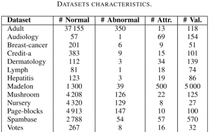
In order to evaluate our approach we use 13 real-world datasets, from the UCI Machine Learning repository [26]. A summary of the information about the datasets is shown in Table III, where we report the number of normal and anomalous instances, the number of attributes and the overall number of different attribute-value pairs. These datasets have been chosen because they exhibit a variety of properties in terms of number of attributes, attribute cardinality and number of objects.
We compare our method with four competitors: LOF (Local Outlier Factor) [10], OSVM (One-Class Support Vector Ma-chine) [14], uLSIF (Unconstrained Least-Square Importance Fitting) [15] and FRaC (Feature Ensemble model) [8]. We use the authors’ implementations of OSVM (in C++), uLSIF (in Octave), FRaC (in Java) and our own implementation of
LOF in Java. SAnDCat is implemented in Java.
To allow LOF working with categorical attributes we need to couple it with a distance function that is able to manage this kind of data. In [24] a comparative study of similarity/distance functions for categorical data is presented. We choose to couple LOF with the Occurrence frequency (OF) distance function because this measure was reported to obtain the highest performance results. This measure assigns a high distance value to mismatches on infrequent values.
For each dataset, we discretized the numerical features using equi-depth bins with the number of bins equal to ten. We
TABLE III
DATASETS CHARACTERISTICS.
Dataset # Normal # Abnormal # Attr. # Val.
Adult 37 155 350 13 118 Audiology 57 1 69 154 Breast-cancer 201 6 9 51 Credit-a 383 9 15 101 Dermatology 112 3 34 139 Lymph 81 1 18 74 Hepatitis 123 3 19 86 Madelon 1 300 39 500 5 000 Mushroom 4 208 126 22 125 Nursery 4 320 129 8 27 Page-blocks 4 913 147 10 100 Spambase 2 788 54 57 570 Votes 267 8 16 32
performed the data pre-processing required by uLSIF and
OSVM and converted each categorical attribute assigning a
boolean attribute to each categorical value (a standard pre-processing for SVM). We adopt the same pre-pre-processing for uLSIF.
The experiments were conducted as follows. Given a dataset, we labeled as normal instances the instances belonging to the majority class (the class with the highest number of instances). Then we selected randomly 3% of instances from the other classes and we label these instances as abnormal. To evaluate the performance of the different semi-supervised approaches we performed a 5-fold cross validation. This means that for each dataset we divided all the instances of the normal class into 5 folds. At each iteration of the cross-validation we learned the model on 4 folds and tested the method on the remaining fold plus the instances of the abnormal class. At the end of the procedure we report the average on the different folds. All the experiments were conducted on a MacBook Pro equipped with a 2.6 GHz Intel Core i5 processor, 8GB RAM and running OS X 10.9.2.
Unfortunately OSVM outlier scores cannot be obtained directly. Thus, in our experiments, the outlier score is the distance from the separating hyperplane, as suggested in [15].
uLSIF is based on a random selection of training instances.
Hence, we ran the algorithm 30 times and we retained the average of the results. Similarly it was done for the RandomK strategy: we averaged its results over 30 runs. Finally, LOF was launched using four different values (10, 20, 30, 40) of the k parameter (the number of neighbors).
A. Evaluation of the results
In Figure 6 we report the results of the first experiment that had the purpose of evaluating the four different strategies em-ployed by SAnDCat for the selection of the k representatives. For each heuristic the value of k ranges over the set: {10, 20, 30, 40}. In Figure 6 we report the average AUC results of SAnDCat on all the datasets. In general the average AUC values are quite high. They vary from a minimum of 0.7568 for the MinDTK method with k = 10, to a maximum of 0.8001 for the MaxDTK method (with k = 40). Interestingly, this method achieves the best results for all the employed values of k. In general, however, the different strategies return similar results, and the value of k does not seem to be much significant
k MinDTK MaxDTK RandomK CentralK 10 0.7568 0.7805 0.7782 0.7654 20 0.7775 0.7966 0.7816 0.7693 30 0.7858 0.799 0.7865 0.7735 40 0.7832 0.8001 0.7877 0.777 (a)
k MinDTK MaxDTK RandomK CentralK
10 2 3 0 0
20 1 1 0 0
30 1 0 0 1
40 1 3 0 0
(b)
Fig. 6. Average AUC (a) and number of wins (b) for all heuristics of SAnDCat and for any given value of k.
for the accuracy of our algorithm. It shows that values of k between 20 and 30 are sufficient to guarantee acceptable anomaly detection rates. Moreover, the differences in AUC for a given heuristic are not significant.
In order to compare our approach with the competitors, we selected the combination of k value and heuristics for
SAnDCat that provides the best average results (that in our
case corresponds with one of the combinations that win most of the times as well). Thus, we select MaxDTK with k = 40. We perform a similar experiment for LOF. We compare the results for k = {10, 20, 30, 40} (see Figure 7) and retain the parameter value which provides the best result (k = 40).
The results of the experiments are reported in Table IV.
SAnDCat wins most of the times (8 datasets over 13). If we
look at the competitors, OSVM wins on three datasets only,
FRaC wins on 4 datasets; uLSIF and LOF never achieve the
best result, but this is not surprising. These two algorithms performs poorly on high-dimensional data, since they are based on density estimation, which is known to work well only on low-dimensional numerical data. Notice that, even when our approach does not win, its AUC is close to the winner’s one. The only exception is constituted by Lymph, but other combination of SAnDCat’s parameters bring to better results for this dataset (e.g., MaxDTK with k = 20 achieves an AUC of 0.8404). These results underline that taking into account the inter-dependence between attributes allows the management of the categorical data and it helps to obtain the best accuracy results for the detection of the anomalous instances. This impression is also confirmed by the average results (see Figure 8) showing that SAnDCat’s average AUC computed on all datasets is sensibly higher than competitors’ ones.
It is worth noting also the poor performance of all al-gorithms when applied to Madelon. In this case, the low AUC values are due to the extremely high dimensionality of the dataset: 500 attributes with 10 values per attribute for a relatively small amount of instances. In these situations, most algorithms are prone to generalization errors.
As additional evaluation, we also perform statistical tests to show the significance of the obtained results. More in detail, we employ the Friedman test [30] based on the average rank
k 10 20 30 40
Avg. AUC 0.3976 0.5067 0.5898 0.6147
No. of wins 1 1 3 8
Fig. 7. LOF’s average AUC and number of wins for any given value of k.
TABLE IV
AUCRESULTS ONUCIDATASETS: SANDCAT VSLOF,ULSIF, OSVM
ANDFRAC.
Dataset SAnDCat LOF uLSIF OSVM FRaC
Adult 0.5743 0.4478 0.3706 0.5961 0.551 Audiology 0.8606 0.8245 0.3595 0.4956 0.4504 Breast-cancer 0.6070 0.5091 0.3624 0.5268 0.5258 Credit-a 0.7494 0.5201 0.3572 0.7317 0.4761 Dermatology 1.0000 0.7857 0.3587 1.0000 1.0000 Hepatitis 0.8860 0.6476 0.3607 0.8136 0.8758 Madelon 0.5063 0.4770 0.2506 0.496 0.5186 Lymph 0.7890 0.8641 0.3635 0.8520 0.8657 Mushroom 0.9995 0.5243 0.3594 0.6730 0.6959 Nursery 1.0000 0.5852 0.3592 0.5667 0.5807 Page-blocks 0.7513 0.2993 0.3626 0.6314 0.6665 Spambase 0.7022 0.4451 0.3383 0.7281 0.7132 Vote 0.9762 0.8979 0.5000 0.9375 0.9942 Avg. AUC 0.8001 0.6021 0.3617 0.6960 0.6856 Std. Dev. 0.1710 0.1868 0.0517 0.1661 0.1927 Max AUC 1.0000 0.8979 0.5000 1.0000 1.0000 Min AUC 0.5063 0.2993 0.2506 0.4956 0.4504 Avg. Rank 1.6154 3.5385 4.9231 2.4615 2.2308
of 5 algorithms on 10 datasets. We compare SAnDCat with all the competitors (FRaC, uLSIF, OSVM, LOF) over all the datasets. The average rank is provided on bottom of Figure IV. According to the Friedman test, the null hypothesis is that all the methods obtain similar performances, i.e., the Friedman statistics X2
F is lower or equal to the critical value of the
chi-square distribution with k − 1 degrees of freedom (k being the number of algorithms). At significance levels of α = 0.01,
X2
F = 29.09 while the critical value of the chi-square
dis-tribution is 13.28. Thus, the null hypothesis is comfortably rejected underling statistically significant differences among the methods. The post-hoc Nemenyi test [30] confirms that, at significance level α = 0.10, our algorithm is the only one that achieves statistically better results w.r.t. the two worst competitors in our experiments, the critical difference being
CDα=0.1= 1.7036.
B. Computational complexity
As we have shown in Section IV-B, the theoretical
com-putational complexity of our algorithm is O(nl2log l) for
training and O(n2) for testing, where l is the number of
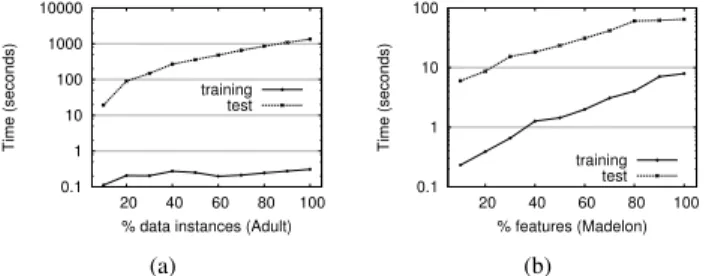
features and n is the number of data objects (assuming that the number of training instances and test instances are of the same order of magnitude). To confirm this theoretical result experimentally, we perform a scalability test by measuring the time performances of SAnDCat (using MaxDTK as heuristic) w.r.t. the number of data instances and features. In details, we consider different percentages (from 10% to 100%) of data instances from Adult, and different percentages (from 10% to 100%) of features from Madelon. Then we train SAnDCat on 80% of the instances and test the remaining 20%. In Figure 9 we report the measured running time for training and test in the two cases. The curves confirm our theoretical analysis.
0 0.2 0.4 0.6 0.8 1
SAnDCat LOF uLSIF OSVM FRaC
Average AUC
Algorithm
Fig. 8. Average AUC results for different Algorithms.
0.1 1 10 100 1000 10000 20 40 60 80 100 Time (seconds)
% data instances (Adult) training test (a) 0.1 1 10 100 20 40 60 80 100 Time (seconds) % features (Madelon) training test (b)
Fig. 9. Runtime of SAnDCat for increasing percentages of instances (left) and features (right).
In particular, training time is mostly affected by dataset dimensionality, while test time strongly depends on dataset size. These results highlight a limitation of our approach: when MaxDTK is chosen as strategy for testing new instances, it is not adapted to online/real-time anomaly detection tasks. However, CentralK and RandK strategies can be used to speed-up the test phase at a reasonable cost in terms of detection accuracy (see Figure 6(a)).
Since the algorithms are implemented in different program-ming languages, we didn’t perform any runtime performance comparison, which would be biased by the specific compiler optimizations and weaknesses. Nonetheless, here we provide a discussion about the theoretical complexity of all the com-petitors.
The only competitor that achieve better theoretical perfor-mances is LOF, whose complexity depends on the nearest neighbors materialization step which requires O(n log n) op-erations [10]. However, when LOF operates on categorical data, it can not leverage any optimized data structure. In this case its complexity is also quadratic. The performances of the other two competitors are in line with those of our algorithm. OSVM involves a complex quadratic programming
problem whose solution requires between O(n2) and O(n3)
operations [14], uLSIF requires a matrix inversion step [15], whose complexity is cubic, even though there exist slightly less complex approximation algorithms. Finally, the complexity of
FRaCdepends on the complexity of the predictors employed
to compute the feature models. Some predictors are linear in the number of data objects (e.g., Naive Bayes), however FRaC
age
ascites
sex
antivirals
spleenPalpable
varices
steroidmalaise anorexia liverBig spiders fatigue liverFirmm histology bilirubin alkPhosphate sgot albumin protime (a)sex
liverBig
antivirals
liverFirm
spleenPalpable
steroid
spiders
varices
fatigue
malaise
ascites
age bilirubin sgot albumin protimeanorexia
(b) agemenopause
irradiat
nodeCaps
degMalig
breast
breastQuad tumorSize invNodes (c) agenodecaps
breast
irradiat
degmalig
menopause
breastquad tumorsize invnodes (d)sex
race
educationNum
workclass fnlwgt maritalStatus relationship capitalGain age education occupation capitalLoss hoursPerWeek (e)sex
maritalstatus
relationship
educationnum
workclass race hoursperweek capitalloss capitalgain education occupation age fnlwgt nativecountry (f)Fig. 10. Attribute clouds for the normal and abnormal classes of Hepatits (a and b), Breast cancer (c and d), and Adult (e and f) employing the attribute model impact.
runs multiple cross-validation loops for each feature and for each classifier of the ensemble, so the complexity may easily
approach O(n2) in some cases.
C. Characterization of anomalies
Here, we show how to inspect the model generated by
SAnDCat with the purpose of understanding the contribution
of each single attribute to the final decision and supporting the usage of visual analytic tools for the exploration of the data. For this experiment, we employ Adult, Breast-cancer and
Hepatitisdatasets. We have chosen these three datasets since
the names of their attributes are self-explaining and may then support a qualitative (rather than quantitative) analysis of the results.
We first employ the attribute impact metric (see Sec-tion IV-C) to obtain visual hints regarding the importance of each attribute. In Figure 10 the word cloud paradigm is adopted in order to provide a graphical representation of the attribute impact.
We observe, for instance, that in Breast cancer attributes menopause, irradiat and nodeCaps have discriminant values for the normal class (patients with no recurrence events, Figure 10(c)), while a variation of these attributes values is less significant for the abnormal class (patients with recurrence events, Figure 10(d)). This means that the values of these particular attributes are homogeneously distributed over all the instances belonging to the abnormal class (therefore they are not predictive of this class). On the other hand, breast,
age
ascites
histology
bilirubin
steroid malaise antivirals albumin protime sex fatigue sgot anorexia liverFirm spleenPalpable spiders alkPhosphate liverBig (a) ageinvNodes
menopause
degMalig
nodeCaps breastQuad breast tumorSize irradiat (b) agesex
educationnum
maritalStatus
fnlwgt
hoursPerWeek workclass education relationship race occupation nativeCountry capitalLoss capitalGain (c)Fig. 11. Attribute clouds for Hepatits(3) (a), Breast cancer(3) (b), and
Adult(3)(c) employing the average attribute distance impact.
the anomalous instances. This change is detected by our algorithm and used to decide whether an instance is normal or anomalous. In Adult, the normal class corresponds to people making less than 50K dollars per year (Figure 10(e)). In this class, the most discriminative attributes are race and sex. In the abnormal class, race is distributed more uniformly, while many other attributes have a more important impact (see Figure 10(f)). Clear variations between the attributes impact are also evidenced in Hepatitis (e.g., see the attribute liverFirm in Figures 10(a) and 10(b)).
In Figure 11 we report the word clouds representing the average attribute distance impact values of the anomalous class. In Adult (we recall again that this dataset has the goal of retaining the people making more than 50K dollars per year, Figure 11(c)), we can observe that race and sex do not contribute much to the distance computation (i.e., the values of these attributes do not differ so much between the normal and anomalous instances). In the case of Hepatitis, the main differences between the anomalous class (died patients, Fig-ure 11(a)) and the normal one (survived patients, FigFig-ure 10(a)) lie in the impact of the attribute histology that does not result so important for the purposes of detecting instances of the normal class while it plays an important role in discriminating between normal and anomalous instances. In the same dataset, we note that the attribute ascites represents a valuable infor-mation because it helps to distinguish normal instances and it is also crucial to discriminate anomalous examples. Similar considerations apply for attributes menopause and invNodes in
Breast cancer as well (see Figure 11(b)).
As a further study, we analyze the discriminative power of
SAnDCatwith respect to the attribute impact. To this purpose,
we rank the attributes in ascending order of I(Xi) and we
retain only top-n features to build the discriminative model. By varying n, we may measure how the attribute impact is related to the accuracy of SAnDCat. The results of these experiments are reported in Figure 13: on the X-axis we report the number of retained attributes, while on the Y-axis we show the achieved AUC. As a general remark, we observe that using half of the attributes in the prediction allows SAnDCat to obtain reasonable and competitive results as with the whole
-0.03 -0.025 -0.02 -0.015 -0.01 -0.005 0 0.005 0.01 0.015 0.02 0.025 -0.015 -0.01 -0.005 0 0.005 0.01 0.015 0.02 0.025 2nd coordinate 1st coordinate Normal Points Abnormal Points (a) -0.1 -0.08 -0.06 -0.04 -0.02 0 0.02 0.04 -0.06 -0.04 -0.02 0 0.02 0.04 0.06 2nd coordinate 1st coordinate Normal Points Abnormal Points (b)
Fig. 12. Test instances visualized using Multi Dimensional Scaling for
Dermatology(a) and Hepatitis (b).
feature space. In some cases using a low number of attributes has a positive impact over the final results. We can observe this phenomenon in Figure 13(c) for SAnDCat applied on Adult. In this case the model built using only 4 to 7 attributes outperforms the model built on the whole attribute space (14 attributes). As a future work, we will study how this selection process can be related to the feature selection task whose goal is the selection of a subset of attributes with the purpose of improving the performance of a classifier [31].
As a final experiment, we employ the MDS (multi-dimensional scaling) technique to plot normal and anomalous data points in a reduced dimensional space. Figure 12 shows the plots obtained by applying a 2-dimensional scaling to the test examples of two datasets: Dermatology and Hepatitis. We observe that the normal instances are well separated from the abnormal ones. Interestingly, some abnormal points are close to each other and they form small clusters in this 2-dimensional representation. A possible application of this technique, is to employ an interactive MDS plot, where the color of each point depends on the outlier score given in Section IV by Equation 3. Thanks to this tool, an analyst may select potential anomalies and inspect them. This tool also supports an active learning process: in fact, the analyst’s feedback on potential anomalies can be used to enrich the positive model, thus providing a more accurate classifier.
In conclusion, while the competitors only aim at the im-provement of the detection performances, SAnDCat not only obtains comparable or better results, but it also supplies
0.00 0.20 0.40 0.60 0.80 1.00 0 2 4 6 8 10 12 14 16 18 20 AUC #Features SAnDCATworst SAnDCATbest (a) 0.00 0.20 0.40 0.60 0.80 1.00 1 2 3 4 5 6 7 8 9 AUC #Features SAnDCATworst SAnDCATbest (b) 0.00 0.20 0.40 0.60 0.80 1.00 0 2 4 6 8 10 12 14 AUC #Features SAnDCATworst SAnDCATbest (c) Fig. 13. AUC for Hepatits (a), Breast cancer (b) and Adult (c), considering only top-k attributes ranked by their impact.
explanatory information that supports an exploratory analysis of the anomalies. Statistical information extracted from the model learnt by SAnDCat can be easily exploited by the user in order to get extra information on how the process works and how it makes its decision.
VI. CONCLUSION
Managing and handling categorical data is a recurrent problem in data mining. Most of the times this kind of data requires ad-hoc techniques in order to obtain satisfactory re-sults. Following this direction, in this paper we have presented a new approach to semi-supervised anomaly detection for categorical data. We have shown that our framework, based on information-theoretic techniques, is able to model categorical data using a distance-based algorithm. We obtain very good results w.r.t. other state-of-the-art semi-supervised methods for anomaly detection. We show that our approach outper-forms also a fully unsupervised anomaly detection technique like LOF that we have coupled with a specific measure for categorical data. We underline also the complementary information that our approach produces during the learning step. In the paper we gave some practical examples of how it is possible to exploit this additional information extracted by our method (distances between instances and the models) in a visualization framework and providing a summary information on the classes.
As a future work we will investigate the following issues: i) new data structures to handle categorical data more efficiently and speed-up the anomaly detection task; ii) new distance-based algorithms that are able to couple the DILCA measure with the usage of feature weights and their employment for data cleaning; iii) a way to extend our analysis in order to manage both continuous and categorical attributes in a unique and more general framework; iv) an extension of the semi-supervised method with active learning.
REFERENCES
[1] V. Chandola, A. Banerjee, and V. Kumar, “Anomaly detection: A survey,” ACM Comput. Surv., vol. 41, no. 3, pp. 15:1–15:58, 2009.
[2] C. Phua, D. Alahakoon, and V. C. S. Lee, “Minority report in fraud detection: classification of skewed data,” SIGKDD Explorations, vol. 6, no. 1, pp. 50–59, 2004.
[3] F. Angiulli and F. Fassetti, “Distance-based outlier queries in data streams: the novel task and algorithms,” Data Min. Knowl. Discov., vol. 20, no. 2, pp. 290–324, 2010.
[4] S. Forrest, S. A. Hofmeyr, A. Somayaji, and T. A. Longstaff, “A sense of self for unix processes,” in Proc. Symp. on Sec. and Privacy, 1996, pp. 120–128.
[5] S. Kasif, S. Salzberg, D. L. Waltz, J. Rachlin, and D. W. Aha, “A probabilistic framework for memory-based reasoning,” Artif. Intell., vol. 104, no. 1-2, pp. 287–311, 1998.
[6] D. Ienco, R. G. Pensa, and R. Meo, “From context to distance: Learning dissimilarity for categorical data clustering,” TKDD, vol. 6, no. 1, p. 1, 2012.
[7] L. Yu and H. Liu, “Feature selection for high-dimensional data: A fast correlation-based filter solution,” in Proc. of ICML, 2003, pp. 856–863. [8] K. Noto, C. E. Brodley, and D. K. Slonim, “Frac: a feature-modeling approach for semi-supervised and unsupervised anomaly detection,” Data Min. Knowl. Discov., vol. 25, no. 1, pp. 109–133, 2012. [9] F. E. Grubbs, “Procedures for detecting outlying observations in
sam-ples,” Technometrics, vol. 11, no. 1, pp. 1–21, February 1969. [10] M. M. Breunig, R. T. N. H-P. Kriegel, and J. Sander, “Lof: identifying
density-based local outliers,” in Proc. of SIGMOD, 2000, pp. 93–104. [11] C.-H. Wang, “Outlier identification and market segmentation using
kernel-based clustering techniques,” Expert Syst. Appl., vol. 36, no. 2, pp. 3744–3750, 2009.
[12] H.-P. Kriegel, M. Schubert, and A. Zimek, “Angle-based outlier detec-tion in high-dimensional data,” in Proc. of KDD, 2008, pp. 444–452. [13] V. Chandola, S. Boriah, and V. Kumar, “A framework for exploring
categorical data,” in Proc. of SDM, 2009, pp. 185–196.
[14] B. Scholkopf, J. C. Platt, J. Shawe-Taylor, A. J. Smola, and R. C. Williamson, “Estimating the support of a high-dimensional distribution,” Neural Computation, vol. 13, p. 2001, 1999.
[15] S. Hido, Y. Tsuboi, H. Kashima, M. Sugiyama, and T. Kanamori, “Sta-tistical outlier detection using direct density ratio estimation,” Knowl. Inf. Syst., vol. 26, no. 2, pp. 309–336, 2011.
[16] V. J. Hodge and J. Austin, “A survey of outlier detection methodologies,” Artif. Intell. Rev., vol. 22, no. 2, pp. 85–126, 2004.
[17] L. Wei, W. Qian, A. Zhou, W. Jin, and J. X. Yu, “Hot: Hypergraph-based outlier test for categorical data,” in Proc. of PAKDD, 2003, pp. 399–410.
[18] Z. He, X. Xu, J. Z. Huang, and S. Deng, “Fp-outlier: Frequent pattern based outlier detection,” Comput. Sci. Inf. Syst., vol. 2, no. 1, pp. 103– 118, 2005.
[19] Z. He, S. Deng, X. Xu, and J. Z. Huang, “A fast greedy algorithm for outlier mining,” in Proc. of PAKDD, 2006, pp. 567–576.
[20] A. Koufakou, E. G. Ortiz, M. Georgiopoulos, G. C. Anagnostopoulos, and K. M. Reynolds, “A scalable and efficient outlier detection strategy for categorical data,” in Proc. of ICTAI (2), 2007, pp. 210–217. [21] K. Das, J. G. Schneider, and D. B. Neill, “Anomaly pattern detection in
categorical datasets,” in KDD, 2008, pp. 169–176.
[22] L. Akoglu, H. Tong, J. Vreeken, and C. Faloutsos, “Fast and reliable anomaly detection in categorical data,” in Proceedings of 21st ACM International Conference on Information and Knowledge Management,
CIKM’12. ACM, 2012, pp. 415–424.
[23] K. Smets and J. Vreeken, “The odd one out: Identifying and char-acterising anomalies,” in Proceedings of the 11th SIAM International
Conference on Data Mining, SDM 2011. SIAM / Omnipress, 2011,
pp. 804–815.
[24] S. Boriah, V. Chandola, and V. Kumar, “Similarity measures for cat-egorical data: A comparative evaluation,” in Proc. of SDM, 2008, pp. 243–254.
[25] R. J. Quinlan, C4.5: Programs for Machine Learning, ser. Morgan
Kaufmann Series in Machine Learning. Morgan Kaufmann, 1993.
[26] C. L. Blake and C. J. Merz, “UCI repository of machine learning databases,” http://www.ics.uci.edu/ mlearn/MLRepository.html, 1998. [27] U. Brandes and C. Pich, “Eigensolver methods for progressive
multidi-mensional scaling of large data,” in Proc. of Graph Drawing, 2006, pp. 42–53.
[28] A. P. Bradley, “The use of the area under the roc curve in the evaluation of machine learning algorithms,” Pattern Recognition, vol. 30, pp. 1145– 1159, 1997.
[29] D. J. Hand and R. J. Till, “A simple generalisation of the area under the roc curve for multiple class classification problems,” Mach. Learn., vol. 45, no. 2, pp. 171–186, 2001.
[30] J. Demsar, “Statistical comparisons of classifiers over multiple data sets,” Jour. of Mach. Lear. Res., vol. 7, pp. 1–30, 2006.
[31] I. Guyon and A. Elisseeff, “An introduction to variable and feature selection,” J. Mach. Learn. Res., vol. 3, pp. 1157–1182, 2003.
Dino Ienco obtained his M.Sc. degree in Computer Science in 2006 and his Ph.D. in Computer Science in 2010, both at the University of Torino. From 2010 to 2011 he had a post-doctoral position at the same University. From February 2011 to September 2011 he was postdoc in Montpellier at Cemagref. Since September 2011 he obtained a permanent position as researcher at the Irstea Institute, Montpellier, France. His research interests are in the areas of data mining and machine learning with particular emphasis on unsupervised techniques (clustering and co-clustering), data stream analysis and spatio-temporal data mining.
Ruggero G. Pensa received the M.Sc. degree in Computer Engineering from the Politecnico of Torino in 2003 and the Ph.D. in Computer Science from INSA of Lyon in 2006. He was adjunct profes-sor at the University of Saint-Etienne (2006-2007); postdoctoral fellows at ISTI-CNR, Pisa (2007-2009); research associate at the University of Torino (2009-2010) and at IRPI-CNR, Torino (2010-2011). Since 2011, he is Assistant Professor at the Department of Computer Science, University of Torino. His main research interests include data mining and knowledge discovery, data science, privacy-preserving algorithms for data management, social network analysis and spatio-temporal data analysis. He served in the programme committee of many international conferences on data mining and machine learning, among which IEEE ICDM, ACM CIKM, SIAM SDM, ECML PKDD, ASONAM.
Rosa Meo took her Master degree in Electronic Engineering in 1993 and her Ph.D. in Computer Science and Systems Engineering in 1997, both at the Politecnico di Torino, Italy. From 2005 she is associate professor at the Department of Computer Science in the University of Torino, where she works in the Database and Data Mining research field. From 2000 to 2003 she was responsible, for the Uni-versity of Torino, of the cInQ Project (consortium on knowledge discovery by Inductive Queries) funded by the V EU Funding Framework. She is active in the field of Database and Data Mining in which she published more than 60 papers. She served in the Programme Committee of many International and National Conferences on Databases and Data Mining, among which VLDB, ACM KDD, IEEE ICDM, SIAM DM, ACM CIKM, ECML/PKDD, ACM SAC, DEXA, DaWak.