HAL Id: hal-01150745
https://hal.archives-ouvertes.fr/hal-01150745v5
Preprint submitted on 6 Feb 2016HAL is a multi-disciplinary open access
archive for the deposit and dissemination of sci-entific research documents, whether they are pub-lished or not. The documents may come from teaching and research institutions in France or abroad, or from public or private research centers.
L’archive ouverte pluridisciplinaire HAL, est destinée au dépôt et à la diffusion de documents scientifiques de niveau recherche, publiés ou non, émanant des établissements d’enseignement et de recherche français ou étrangers, des laboratoires publics ou privés.
Local Error Estimates of the Finite Element Method for
an Elliptic Problem with a Dirac Source Term
Silvia Bertoluzza, Astrid Decoene, Loïc Lacouture, Sébastien Martin
To cite this version:
Silvia Bertoluzza, Astrid Decoene, Loïc Lacouture, Sébastien Martin. Local Error Estimates of the Finite Element Method for an Elliptic Problem with a Dirac Source Term. 2015. �hal-01150745v5�
Local Error Estimates of the Finite Element Method
for an Elliptic Problem with a Dirac Source Term
Silvia BERTOLUZZA, Astrid DECOENE, Lo¨ıc LACOUTURE and S´ebastien MARTIN February 3, 2016
Abstract: The solutions of elliptic problems with a Dirac measure right-hand side are not H1 and therefore the convergence of the finite element solutions is suboptimal. The use of graded meshes is standard remedy to recover quasi-optimality, namely optimality up to a log-factor, for low order finite elements in the L2
-norm. Optimal (or quasi-optimal for the lowest order case) convergence for Lagrange finite elements has been shown, in the L2
-norm, on a subdomain which excludes the singularity. Here, on such subdomains, we show a quasi-optimal convergence in the Hs-norm, for sě 1, and, in the particular case of Lagrange finite elements, an optimal convergence
in H1
-norm, on a family of quasi-uniform meshes in dimension 2. The study of this problem is motivated by the use of the Dirac measure as a reduced model in physical problems, for which high accuracy of the finite element method at the singularity is not required. Our results are obtained using local Nitsche and Schatz-type error estimates, a weak version of Aubin-Nitsche duality lemma and a discrete inf-sup condition. These theoretical results are confirmed by numerical illustrations.
Key words: Dirichlet problem, Dirac measure, Green function, finite element method, local error estimates.
1
Introduction.
This paper deals with the accuracy of the finite element method on elliptic problems with a singular right-hand side. More precisely, let us consider the Dirichlet problem
pPδq
"
´△uδ “ δx0 in Ω,
uδ “ 0 onBΩ,
where Ω Ă R2
is a bounded open C8 domain or a square, and δ
x0 denotes the Dirac measure
concentrated at a point x0 P Ω such that distpx0,BΩq ą 0.
Problems of this type occur in many applications from different areas, like in the mathematical modeling of electromagnetic fields [17]. Dirac measures can also be found on the right-hand side of adjoint equations in optimal control of elliptic problems with state constraints [8]. As further examples where such measures play an important role, we mention controllability for elliptic and parabolic equations [9,10,21] and parameter identification problems with pointwise measurements [23].
Our interest in pPδq is motivated by the modeling of the movement of a thin structure in a
viscous fluid, such as cilia involved in the muco-ciliary transport in the lung [15]. In the asymptotic of a zero diameter cilium with an infinite velocity, the cilium is modelled by a line Dirac of force in the source term. In order to make the computations easier, the line Dirac can be approximated by
a sum of punctual Dirac forces distributed along the cilium [20]. In this paper, we address a scalar version of this problem: problem pPδq.
In the regular case, namely the Laplace problem with a regular right-hand side, the finite element solution uh is well-defined and for uP Hk`1pΩq, we have, for all 0 ď s ď 1,
}u ´ uh}sď Chk`1´s}u}k`1, (1)
where k is the degree of the method [11] and h the mesh size. In dimension 1, the solution uδ of
Problem pPδq belongs to H1pΩq, but it is not H2pΩq. In this case, the numerical solution uhδ and
the exact solution uδ can be computed explicitly. If x0 coincides with a node of the discretization,
uhδ “ uδ. Otherwise, this equality holds only on the complementary of the element which contains x0,
and the convergence orders in H1
-norm and L2
-norm are 1/2 and 3/2 respectively. In dimension 2, ProblempPδq has no H1pΩq-solution, and so, although the finite element solution can be defined, the
H1
pΩq-error makes no sense and the L2
pΩq-error estimates cannot be obtained by a straightforward application of the Aubin-Nitsche method.
Let us review the literature on error estimates for problem pPδq, starting with discretizations
on quasi-uniform meshes. Babu˜ska [4] showed an L2
pΩq-convergence of order h1´ε, ε ą 0, for a
two-dimensional smooth domain. Scott proved in [25] an a priori error estimate of order 2´ d2, where the dimension d is 2 or 3. The same result has been proved by Casas [7] for general Borel measures on the right-hand side.
To the best of our knowledge, in order to improve the convergence order, Eriksson [14] was the first who studied the influence of locally refined meshes near x0. Using results from [24], he
proved convergence of order k and k` 1 in the W1,1pΩq-norm and the L1
pΩq-norm respectively, for approximations with a Pk-finite element method. Recently, by Apel and co-authors [2], an
L2pΩq-error estimate of order h2| ln h|3{2 has been proved in dimension 2, using graded meshes. Optimal convergence rates with graded meshes were also recovered by D’Angelo [12] using weighted Sobolev spaces. A posteriori error estimates in weighted spaces have been established by Agnelli and co-authors [1].
These theoretical a priori results are based upon graded meshes, which increase the complexity of the meshing and the computational cost, even if the mesh is refined only locally, especially when the right-hand side includes several Dirac measures, that can be static or moving. Therefore Eriksson [13] developped a numerical method to solve the problem and recovers the optimal convergence rate: the numerical solution is searched in the form u0` vh where u0 contains the singularity of the
solution and vh is the numerical solution of a smooth problem. This method has been developped
in the case of the Stokes problem in [20].
However, in applications, the Dirac measure at x0 is often a model reduction approach, and a
high accuracy at x0 of the finite element method is not necessary. Thus, it is interesting to study
the error on a fixed subdomain which excludes the singularity. Recently, K¨oppl and Wohlmuth have shown in [19] optimal convergence in L2
-norm for the Lagrange finite elements (the result is quasi-optimal for the P1
-element). In this paper, we consider the problem in dimension 2, and we show :
1. Quasi-optimal convergence in Hs-norm, for sě 1. This result applies to a wide class of
finite-element methods and beyond, including Lagrange and Hermite finite finite-elements and wavelets. The L2-error estimates established in [19] are not used and the proof is based on different arguments.
2. Optimal convergence in H1
-norm for the Lagrange finite elements. This result is obtained by direct use of the optimal L2
-norm convergence result in [19]. 3. Optimal convergence in H1
-norm in the particular case of the P1
-Lagrange finite element using different arguments than those used for the previous results.
These results imply that graded meshes are not required to recover optimality far from the singularity and that there are no pollution effects. In addition, by linearity of Problem pPδq, the
result holds in the case of several Dirac masses. The paper is organized as follows. Our main results are presented in Section 2 after recalling the Nitsche and Schatz Theorem, which is an important tool for the proof presented in Section 3. In Section 4 another argument is presented to obtain an optimal estimate in the particular case of the P1-finite elements. We illustrate in Section 5 our
theoretical results by numerical simulations and, in Section 6, we discuss the generalization of our approach to the three-dimensional case.
2
Main results.
In this section, we define all the notations used in this paper, formulate our main results and recall an important tool for the proof, the Nitsche and Schatz Theorem.
2.1 Notations. x0 Ω Ω0 Ω1 BΩ0 BΩ 1 mesh
Figure 1: Domains Ω0 and Ω1.
For a domain D, we will denote by } ¨ }s,p,D (respectively| ¨ |s,p,D) the norm (respectively the
semi-norm) of the Sobolev space Ws,ppDq, while } ¨ }
s,D (respectively | ¨ |s,D) will stand for the norm
(respectively the semi-norm) of the Sobolev space HspDq.
For the numerical solution, let us introduce a family of quasi-uniform simplicial triangulations Th of Ω and an order k finite element space Vk
h Ă H 1
0pΩq. To ensure that the numerical solution
is well-defined, the space Vk
h is assumed to contain only continuous functions. The finite element
solution uh
δ P Vhk of problempPδq is defined by
ż
Ω
∇uhδ¨ ∇vh “ vhpx0q, @vh P Vhk. (2)
For s ě 2, we will also evaluate the Hs-norm of the error on a subdomain of Ω which does not
contain the singularity, and, whenever we do so, we will of course assume the finite elements to be Hs-conforming. We fix two subdomains Ω
0 and Ω1 of Ω, such that Ω0 ĂĂ Ω1 ĂĂ Ω and x0 R Ω1
Assumption 1. For some h0, we have for all 0ă h ď h0 (see Figure 1), Ωm0 ŞΩc1“ H, where Ω m 0 “ ď TPTh TŞΩ0‰H T, and Ωc 1 is the complement of Ω1 in Ω.
2.2 Regularity of the solution uδ.
In this subsection, we focus on the singularity of the solution, which is the main difficulty in the study of this kind of problems. In dimension 2, problem pPδq has a unique variational solution
uδP W 1,p
0 pΩq for all p P r1, 2r (see for instance [3]). Indeed, denoting by G the Green function, G is
defined by
Gpxq “ ´ 1
2π logp|x|q.
This function G satisfies´△G “ δ0, so that Gp¨ ´ x0q contains the singular part of uδ. As it is done
in [3], the solution uδ can be built by adding to Gp¨ ´ x0q a corrector term ω P H1pΩq, solution of
the Laplace( problem "
´△ω “ 0 in Ω,
ω “ ´Gp¨ ´ x0q on BΩ. (3)
Then, the solution is given by
uδpxq “ Gpx ´ x0q ` ωpxq “ ´
1
2π logp|x ´ x0|q ` ωpxq.
It is easy to verify that uδ R H01pΩq. Actually, we can specify how the quantity }uδ}1,p,Ω goes
to infinity when p goes to 2, with p ă 2. According to the foregoing, if we write uδ “ G ` ω,
since ωP H1
pΩq, estimating the behavior of }uδ}1,p,Ωas p converges to 2 from below (which will be
denoted by p Õ 2) is reduced to estimating the behavior }G}1,p,B, where B “ Bp0, 1q where B is
the ball of center 0 and radius 1. GP LppΩq for all 1 ď p ă 8, and using polar coordinates, we get, for pă 2, |G|p1,p,B “ ż B|∇Gpxq| pdx “ ż1 0 ż2π 0 ˆ 1 2π 1 r ˙p rdθdr“ p2πq1´p ż1 0 r1´pdr“ p2πq 1´p 2´ p . Finally, when pÕ 2, }uδ}1,p,Ω„ 1 ? 2π 1 ? 2´ p. (4)
2.3 The Nitsche and Schatz Theorem.
Before stating the Nitsche and Schatz Theorem, let us introduce some known properties of the finite element spaces Vk
h.
Assumption 2. Given two fixed concentric spheres B0 and B with B0 ĂĂ B ĂĂ Ω, there exists
an h0 such that for all 0ă h ď h0, we have for some Rě 1 and M ą 1:
B1 For any 0ď s ď R and s ď ℓ ď M, for each u P HℓpBq, there exists η P Vk
h such that
}u ´ η}s,B ď Chℓ´s}u}ℓ,B.
Moreover, if uP H1
B2 Let ϕP C8
0 pB0q and uhP Vhk, then there exists ηP Vhk
ŞH1
0pBq such that
}ϕuh´ η}1,B ď Cpϕ, B, B0qh}uh}1,B.
B3 For each hď h0 there exists a domain Bh with B0 ĂĂ Bh ĂĂ B such that if 0 ď s ď ℓ ď R
then for all uh P Vhk we have
}uh}ℓ,Bh ď Ch s´ℓ
}uh}s,Bh.
We now state the following theorem, a key tool in the forthcoming proof of Theorem1.
Theorem (Nitsche and Schatz [22]). Let Ω0 ĂĂ Ω1 ĂĂ Ω and let Vhk satisfy Assumption 2. Let
uP HℓpΩ1q, let uh P Vhk and let q be a nonnegative integer, arbitrary but fixed. Let us suppose that
u´ uh satisfies ż
Ω
∇pu ´ uhq ¨ ∇vh “ 0, @vh P VhkŞH01pΩ1q.
Then there exists h1 such that if hď h1 we have
(i) for s“ 0, 1 and 1 ď ℓ ď M,
}u ´ uh}s,Ω0 ď C
´
hℓ´s}u}ℓ,Ω1 ` }u ´ uh}´q,Ω1
¯ ,
(ii) for 2ď s ď ℓ ď M and s ď k ă R, }u ´ uh}s,Ω0 ď C ´ hℓ´s}u}ℓ,Ω1 ` h 1´s }u ´ uh}´q,Ω1 ¯ .
In this paper, we will actually need a more general version of the assumptions on the approxi-mation space Vk
h:
Assumption 3. Given B Ă Ω, consider p1 ě 2, there exists an h0 such that for all 0ă h ď h0, we
have for some Rě 1 and M ą 1: r
B1 For any 0 ď s ď R and s ď ℓ ď M, for each u P HℓpBq, there exists η P Vk
h such that, for
any finite element T Ă B,
|u ´ η|s,p1,T ď Chdp1{p 1
´1{2qhℓ´s
|u|ℓ,2,T.
r
B3 For 0ď s ď ℓ ď R, for all uh P Vhk, for any finite element T in the family Th, we have
}uh}ℓ,p1,T ď Chdp1{p 1
´1{2qhs´ℓ}u h}s,2,T.
Assumptions rB1and rB3are generalizations of assumptions B1 and B3. They are quite standard and satisfied by a wide variety of approximation spaces, including all finite element spaces defined on quasi-uniform meshes [11]. The parameters R and M play respectively the role of the regularity and order of approximation of the approximation space Vk
h. For example, in the case of P1-finite
elements, we have R“ 3{2 ´ ε and M “ 2. Assumption B2 is less common but also satisfied by a wide class of approximation spaces. Actually, for Lagrange and Hermite finite elements, a stronger property than assumption B2 is shown in [5]: let 0ď s ď ℓ ď k, ϕ P C8
0 pBq and uh P Vhk, then
there exists η P Vhk such that
}ϕuh´ η}s,B ď Cpϕqhℓ´s`1}uh}ℓ,B. (5)
2.4 Statement of our main results.
Our main results are Theorems 1,2 and3. The rest of the paper is mostly concerned by the proof and the numerical illustration.
Theorem 1. Let Ω0 ĂĂ Ω1 ĂĂ Ω satisfy Assumption 1, 1 ď s ď k. Let uδ be the solution of
problem pPδq and uhδ its Galerkin projection onto Vhk, satisfying (2). Under Assumptions 2 and 3,
there exists h1 such that if 0ă h ď h1, we have,
}uδ´ uhδ}1,Ω0 ď CpΩ0,Ω1,Ωqhk
a
| ln h|. (6)
In addition, for sě 2, if the finite elements are supposed Hs-conforming, we have
}uδ´ uhδ}s,Ω0 ď CpΩ0,Ω1,Ωqhk`1´s
a
| ln h|. (7)
Remark 1. The main tool in proving Theorem 1is the Nitsche and Schatz Theorem, and the result holds for all the spaces verifying Assumptions 2 and 3. The class of such spaces includes spaces beyond finite elements, including, for instance, wavelets.
Section3 will be dedicated to the proof of Theorem1.
In the particular case of Lagrange finite elements, K¨oppl and Wohlmuth [19] showed, in the L2-norm of a subdomain which does not contain x0, quasi-optimality for the lowest order case, and optimal a priori estimates for higher order. The proof is based on Wahlbin-type arguments, which are similar to the Nitsche and Schatz Theorem (see [27,28]), and different arguments from the ones presented in this paper, like the use of an operator of Scott and Zhang type [26]. Using this result it is possible to prove quite easily optimal convergence in H1
-norm for Lagrange finite elements. This result reads as follows:
Theorem 2. Consider a domain Ω2 such that Ω0 ĂĂ Ω1 ĂĂ Ω2 ĂĂ Ω, x0 R Ω2, and satisfying
Assumption 1. Let uδ be the solution of problempPδq and uhδ its Galerkin projection onto the space
of Lagrange finite elements of order k` 1. There exists h1 such that if 0ă h ď h1, we have
}uδ´ uhδ}1,Ω0 ď CpΩ1,Ω2,Ωqhk. (8)
Remark 2. This result is optimal and thus slightly stronger than inequality (6), but it is limited to Lagrange finite elements and to the H1
-norm, due to the use of an operator of Scott-Zhang type. Theorem 1 is more general: it holds for a wide class of finite elements and it allows to estimate the error in Hs-norm, for any sě 1.
Proof of Theorem 2. In the particular case of Lagrange finite elements, K¨oppl and Wohlmuth proved in [19] the following convergence in the L2
-norm of a subdomain which does not contain x0:
}uδ´ uhδ}0,Ω1 ď CpΩ1,Ω2,Ωq
" h2
| lnphq| if k “ 1,
hk`1 if ką 1. (9)
Let us apply the Nitsche and Schatz Theorem on Ω0 and Ω1 for l“ k ` 1 and q “ 0,
}uδ´ uhδ}1,Ω0 ď C ´ hk}uδ}2,Ω1` }uδ´ uhδ}0,Ω1 ¯ . Using (9), we get }uδ´ uhδ}1,Ω0 ď Chk.
For the particular P1-Lagrange finite elements, we prove the optimal convergence in H1-norm
using completely different arguments. This proof involves a technical assumption on the mesh, namely Assumption 4 in Section 4.2: the distance of the Dirac mass to the edges of the mesh triangles is assumed to be at least of the same order as the mesh size h. The result reads as follows:
Theorem 3. Let Ω0ĂĂ Ω1 ĂĂ Ω satisfy Assumption1 and consider a mesh such that there exists
a domain Bε satisfying Assumption 4 with ǫ of the same order as the mesh size. The P1-finite
element method converges with order 1 for the H1
pΩ0q-norm. More precisely:
}uδ´ uhδ}1,Ω0 ď CpΩ0,Ω1,Ωqh.
The proof of this result is detailed in Section 4.
3
Proof of Theorem
1
.
This section is devoted to the proof of Theorem 1. We first show a weak version of the Aubin-Nitsche duality lemma (Lemma 1) and establish a discrete inf-sup condition (Lemma 2). Then, we use these results to prove Theorem 1.
3.1 Aubin-Nitsche duality lemma with a singular right-hand side.
The proof of Theorem 1 is based on the Nitsche and Schatz Theorem of Section 2.3. In order to estimate the quantity }uδ´ uhδ}´q,Ω1, we will first show a weak version of Aubin-Nitsche Lemma,
for the case of Poisson Problem with a singular right-hand side. Lemma 1. Let f P W´1,ppΩq “ pW1,p1
0 pΩqq1, 1ă p ă 2, and u P W 1,p
0 pΩq be the unique solution of
"
´△u “ f in Ω, u “ 0 on BΩ.
Let uh P Vhk be the Galerkin projection of u. For finite elements of order k, letting e“ u ´ uh, we
have for all 0ď q ď k ´ 1,
}e}´q,Ωď Chq`1h2p1{p 1
´1{2q|e|
1,p,Ω. (10)
Proof. We aim at estimating, for q ě 0, the H´q-norm of the error e:
}e}´q,Ω“ sup φPC8 0 pΩq |şΩeφ| }φ}q,Ω . (11)
The error eP W01,p satisfies ż
Ω
∇e¨ ∇vh “ 0, @vh P Vhk.
Consider φP C08pΩq and let wφP Hq`2 be the solution of
"
´△wφ “ φ in Ω,
wφ “ 0 on BΩ.
In dimension 2, by the Sobolev injections established for instance in [6], Hq`2pΩq Ă W1,p1
pΩq for all p1 inr2, `8r. Thus, for any wh P Vhk,
ˇ ˇ ˇ ˇ ż Ω eφ ˇ ˇ ˇ ˇ “ ˇ ˇ ˇ ˇ ż Ω e△wφ ˇ ˇ ˇ ˇ “ ˇ ˇ ˇ ˇ ż Ω ∇e¨ ∇wφ ˇ ˇ ˇ ˇ “ ˇ ˇ ˇ ˇ ż Ω ∇e¨ ∇pwφ´ whq ˇ ˇ ˇ ˇ ď |wφ´ wh|1,p1,Ω|e|1,p,Ω. We have to estimate |wφ´ w h|1,p1,Ω. It holds |wφ´ wh|p 1 1,p1,Ω“ ÿ T |wφ´ wh|p 1 1,p1,T.
For all 0 ď q ď k ´ 1 and for all element T in Th, thanks to Assumption rB1 applied for s “ 1,
ℓ“ q ` 2, there exists whP Vhk such as
|wφ´ wh|1,p1,T ď Ch 2p1{p1
´1{2qhq`1|wφ
|q`2,2,T. (12)
We number the triangles of the meshtTi, i“ 1, ¨ ¨ ¨ , Nu and we set
a“ paiqi and b“ pbiqi, where ai “ |wφ´ wh|1,p1,Ti and bi “ |wφ|q`2,2,Ti.
By (12), we have, for all i in rr1, Nss,
ai ď Ch2p1{p 1
´1{2qhq`1b i.
We recall the norm equivalence in RN for 0ă r ă s,
}x}ℓs ď }x}ℓr ď N1{r´1{s}x}ℓs.
Remark that here N „ Ch´2. As 2ă p1, we have }b}ℓp1 ď }b}ℓ2. Then, we can write
|wφ´ wh|1,p1,Ω“ }a} ℓp1 ď Chq`1h 2p1{p1 ´1{2q}b} ℓp1 ď Chq`1h2p1{p1´1{2q}b}ℓ2 ď Chq`1h2p1{p1´1{2q|wφ|q`2,2,Ω ď Chq`1h2p1{p1´1{2q}φ}q,Ω.
Finally, using this estimate in (11), we obtain, for q ď k ´ 1, }e}´q,Ωď Chq`1h2p1{p
1 ´1{2q
|e|1,p,Ω.
Corollary 1. For finite elements of order k, for any 0ă ε ă 1,
}uδ´ uhδ}´k`1,Ωď Chkh´ε|uδ´ uhδ|1,p,Ω, (13) where pPs1, 2r is defined by p“ 2 1` ε ˆ and so p1 “ 2 1´ ε ˙ . (14)
Proof. We will apply Lemma1to estimate}uδ´uhδ}´q,Ωforpp, p1q defined in (14). In inequality (10):
2 ˆ 1 p1 ´ 1 2 ˙ “ 2 ˆ 1´ ε 2 ´ 1 2 ˙ “ ´ε. (15)
Finally, for finite elements of order k,
3.2 Estimate of |uδ´ uhδ|1,p,Ω.
It remains to estimate the quantity |uδ´ uhδ|1,p,Ω by bounding|uhδ|1,p,Ωin terms of|uδ|1,p,Ω(equality
(17)). To achieve this, we will need the following discrete inf-sup condition.
Lemma 2. For 0ă ε ă 1, p and p1 defined in (14), we have the discrete inf-sup condition
inf uhPVk h sup vhPVk h ş Ω∇uh¨ ∇vh }uh}1,p,Ω}vh}1,p1,Ω ě Ch ε.
Proof. The continuous inf-sup condition inf uPW01,p sup vPW01,p1 ş Ω∇u¨ ∇v }u}1,p}v}1,p1 ě β ą 0
holds for β independent of p and p1 (and thus independent of ε). It is a consequence of the duality of the two spaces W01,ppΩq and W
1,p1
0 pΩq, see [18]. For vP W 1,p1
0 pΩq, let Πhvdenote the H01-Galerkin
projection of v onto Vk
h. This is well defined since W 1,p1
0 pΩq Ă H 1
0pΩq. We apply Assumption rB3
to Πhv for ℓ“ s “ 1, and get
}Πhv}1,p1,Ωď Ch´2p1{2´1{p 1 q }Πhv}1,2,Ωď Ch´2p1{2´1{p 1 q }v}1,2,Ωď Ch´2p1{2´1{p 1 q }v}1,p1,Ω.
Moreover, for any uh P VhkĂ W 1,ppΩq, }uh}1,p,Ωď C sup vPW01,p1 ş Ω∇uh¨ ∇v }v}1,p1,Ω “ C sup vPW01,p1 ş Ω∇uh¨ ∇Πhv }v}1,p1,Ω ď Ch´2p1{2´1{p1q sup vPW01,p1 ş Ω∇uh¨ ∇Πhv }Πhv}1,p1,Ω ď Ch´2p1{2´1{p1q sup vhPVk h ş Ω∇uh¨ ∇vh }vh}1,p1,Ω .
Finally, thanks to Poincar´e inequality, and to inequality (15),
inf uhPVk h sup vhPVk h ş Ω∇uh¨ ∇vh }uh}1,p,Ω}vh}1,p1,Ω ě Ch ε.
Then, we can estimate |uδ´ uhδ|1,p,Ω :
Lemma 3. With p and p1 defined in (14),
|uδ´ uhδ|1,p,Ωď C
h´ε
?ε. (16)
Proof. According to Lemma 2, it exists vh P Vhk, with}vh}1,p1,Ω“ 1, such that
h2p1{2´1{p1q}uhδ}1,p,Ωď C ż Ω ∇uhδ ¨ ∇vh“ C ż Ω ∇uδ¨ ∇vh ď C}uδ}1,p,Ω. So we have |uδ´ uhδ|1,p,Ωď |uδ|1,p,Ω` |uhδ|1,p,Ωď Ch´2p1{2´1{p 1 q }uδ}1,p,Ω. (17)
All that remains is to substitute }uδ}1,p,Ω for the expression established in (4). For p defined as in (14), }uδ}1,p,Ωď C ? 2´ p ď C ?ε. Finally, with (15) and (17), we get
|uδ´ uhδ|1,p,Ωď C
h´ε ?ε.
3.3 Proof of Theorem 1. We can now prove Theorem 1.
Proof. The function uδis analytic on Ω1, therefore the quantity}uδ}k`1,Ω1 is bounded. If we suppose
s“ 1, Nitsche and Schatz Theorem gives, for ℓ “ k ` 1 and q “ k ´ 1, }uδ´ uhδ}1,Ω0 ď C ´ hk` }uδ´ uhδ}´k`1,Ω1 ¯ . Thanks to (13) and (16), }uδ´ uhδ}´k`1,Ωď Chk h´2ε ? ε , therefore, taking ε“ | ln h|´1, }uδ´ uhδ}´k`1,Ωď Chk a | ln h|. (18)
Finally, we get the result of Theorem 1 for s“ 1 (inequality (6)): }uδ´ uhδ}1,Ω0 ď Chk
a | ln h|.
Now, let us fix 2ď s ď k, Nitsche and Schatz Theorem gives, for ℓ “ k ` 1 and q “ k ´ 1, }uδ´ uhδ}s,Ω0 ď C
´
hk`1´s` h1´s}uδ´ uhδ}´k`1,Ω1
¯ .
So, thanks to (18), we get the second result of Theorem1(inequality (7)), }uδ´ uhδ}s,Ω0 ď Chk`1´s
a | ln h|. which ends the proof of Theorem 1.
4
Proof of Theorem
3
.
To prove this theorem, we first regularize the right-hand side, and prove that in our case the solution uδ of pPδq and the solution of the regularized problem coincide on the complementary of a
neighborhood of the singularity (Theorem 4). The proof of Theorem 3is based, once again, on the Nitsche and Schatz Theorem and on the observation that the discrete right-hand sides of problem pPδq and of the regularized problem are exactely the same, so that the numerical solutions are the
4.1 Direct problem and regularized problem.
The results presented in this section are valid in any dimension d ě 1. However they will only be applied in dimension 2 in Section 4.3 in order to prove Theorem 2. Let εą 0, and fεbe defined on
Ω by
fε“
d
σpSd´1qεd1Bε
, (19)
where Bε “ Bpx0, εq and σpSd´1q is the Lebesgue measure of the unit sphere in dimension d. The
parameter ε is supposed to be small enough so that Bε ĂĂ Ω. The function fε is a regularization
of the Dirac distribution δx0. Let us consider the following problem:
pPεq
"
´△uε “ fε in Ω,
uε “ 0 on BΩ.
Since fε P L2pΩq, it is possible to show that problem pPεq has a unique variational solution uε in
H1
0pΩqŞH 2
pΩq [16]. We will show the following result:
Theorem 4. The solution uδ of pPδq and the solution uε of pPεq coincide on rΩ“ ΩzBε, ie,
uδ| r
Ω “ uε|Ωr
.
The proof is based on the following lemma.
Lemma 4. Let d P Nzt0u, ε ą 0, x P Rd, v a function defined on Rd, harmonic on Bpx, εq, and
f P L1pRdq such that
• f is radial and positive, • supppf q Ă Bp0, εq, ε ą 0, • ż Rd fpxq dx “ 1. Then, f˚ vpxq “ ż Rd fpyqvpx ´ yq dy “ vpxq.
Proof. As supppf q Ă Bp0, εq, using spherical coordinates, we have: f˚ vpxq “ żε 0 ż Sd´1 fprqvpx ´ rωqrd´1dω dr“ żε 0 rd´1fprq ˆż Sd´1 vpx ´ rωqdω ˙ dr.
Besides, v is harmonic on Bpx, εq, so that the mean value property gives, for 0 ă r ď ε, vpxq “ 1 σpBBpx, rqq ż BBpx,rq vpyq dy “ r d´1 σpBBpx, rqq ż Sd´1 vpx ´ rωq dω, thus f ˚ vpxq “ żε 0 fprqvpxqσpBBpx, rqq dr “ vpxq żε 0 ż Sd´1 fprqrd´1dω dr“ vpxq ż Bp0,εq fpyq dy “ vpxq.
Proof. First, let us leave out boundary conditions and consider the following problem
´ △u “ fε in D1pRdq. (20)
As ´△G “ δ0 in D1pRdq, we can build a function u satisfying (20) as:
upxq “ fε˚ Gpxq “ ż Rd fεpyqGpx ´ yq dy “ ż Rd fεpx0` yqGpx ´ x0´ yq dy “ ´ fεpx0` ¨q ˚ G ¯ px ´ x0q.
Moreover, for all xP ΩzBε, G is harmonic on Bpx ´ x0, εq, and fεp¨ ` x0q satisfies the assumptions
of Lemma4, so that upxq “´fεpx0` ¨q ˚ G
¯
px ´ x0q “ Gpx ´ x0q. We conclude that u and Gp¨ ´ x0q
have the same trace on BΩ, and so u ` ω, where ω is the solution of the Poisson problem (3), is a solution of the problempPεq. By the uniqueness of the solution, we have uε“ u ` ω. Finally, for all
x P ΩzBε, uεpxq “ uδpxq. Since these functions are continuous on rΩ“ ΩzBε, this equality is true
on the closure of rΩ, which ends the proof of Theorem4.
Remark 3. Theorem 4 holds for any radial positive function f P L1
pRdqŞL2 pRdq such that supppf q Ă Bp0, εq and ż Rd fpxq dx “ 1, taking fε“ f p¨ ´ x0q. It is a direct consequence of Lemma 4.
Remark 4. Theorem 4 is true in dimension 1, taking fε“
1
2ε1Iε, where Iε “ rx0´ ε, x0 ` εs Ă sa, br“ I. In this case, we can easily write down the solutions uδ and uε explicitly,
uδpxq “ $ ’ ’ & ’ ’ % b´ x0 b´ a x´ a b´ x0 b´ a if xP ra, x0s, ´xb0´ a ´ a x` b x0´ a b´ a if xP rx0, bs. uεpxq “ $ ’ ’ ’ ’ ’ ’ ’ ’ ’ ’ ’ ’ ’ ’ ’ ’ & ’ ’ ’ ’ ’ ’ ’ ’ ’ ’ ’ ’ ’ ’ ’ ’ % b´ x0 b´ a x´ a b´ x0 b´ a if xP ra, x0´ εs, ´x 2 4ε ` ˆ x0 2ε ` a` b ´ 2x0 2pb ´ aq ˙ x `apx0´ bq ` bpx2 0´ aq pb ´ aq ´ x20` ε 2 4ε if xP rx0´ ε, x0` εs, ´xb0´ a ´ a x` b x0´ a b´ a if xP rx0` ε, bs. and observe, as shown in Figure 2, that uδ and uε coincide outside Iε.
a b uδ
uε
x0´ ε x0 x0` ε
Figure 2: Illustration of Theorem4 in 1D.
4.2 Discretizations of the right-hand sides.
At this point, we introduce a technical assumption on Bε and the mesh.
Assumption 4. The domain of definition Bε of the function fε is supposed to satisfy
Bε Ă T0,
where T0 denotes the triangle of the mesh which contains the point x0 (Figure 3).
T0
Bε
Figure 3: Assumption on Bε.
Remark 5. The parameter ε will be chosen to be h{10, so it remains to fix a “good” triangle T0 and
to build the mesh accordingly, so that Assumption 4 is satisfied. Remark that it is always possible to locally modify any given mesh so that it satisfies this assumption.
Lemma 5. Under Assumption 4,
uhε “ uhδ, where uh
Proof. Let us write down explicitly the discretized right-hand side Fh
ε associated to the function
fε: for all node i and associated test function vi P Vh1,
` Fεh˘i“ ż Ω 1 σpBεq1Bεpxqvipxq dx “ ż BεĂT0 1 σpBεq vipxq dx,
and vi is affine (and so harmonic) on T0, therefore
`
Fεh˘i “ "
vipx0q if i is a node of the triangle T0,
0 otherwise. We note that Fh
ε “ Dh, where Dh is the discretized right-hand side vector associated to the Dirac
mass. That is why, with Ah the Laplacian matrix,
uhε ´ uhδ “ ÿ
i node
”
A´1h `Fεh´ Dh˘ı
ivi“ 0.
Remark 6. Fεh “ Dh holds as long as BεĂ T0. Otherwise, we still have uδ|Ω0 “ uε|Ω0 (Theorem
4), but Fh
ε ‰ Dh, and so uhδ|Ω ‰ u h ε|Ω.
4.3 Proof of Theorem 3. Theorem 3can now be proved.
Proof. First, by triangular inequality, we can write, for sP t0, 1u:
}uδ´ uhδ}s,Ω0 ď }uδ´ uε}s,Ω0` }uε´ uhε}s,Ω0 ` }uhε ´ uhδ}s,Ω0.
Besides, thanks to Theorem4, we have
}uδ´ uε}s,Ω0 “ 0, (21)
and thanks to Lemma 5, we have
}uhδ ´ uhε}s,Ω0 “ 0.
Finally we get
}uδ´ uhδ}s,Ω0 ď }uε´ uhε}s,Ω0. (22)
We will apply the Nitsche and Schatz Theorem to e“ uε´ uhε. With ℓ“ 2, s “ 1, and p “ 0,
}e}1,Ω0 ď C ph}uε}2,Ω1` }e}0,Ω1q . (23)
The domain Ω is smooth and fε P L2pΩq, so uε P H2pΩqŞH01pΩq, and then, thanks to inequality
(1), }e}0,Ω1 ď }e}0,Ωď Ch 2 }uε}2,Ωď Ch 2 }fε}0,Ω.
As }fε}0,Ω can be computed exactely,
}fε}0,Ω“ ˜ż Ω ˆ 1 πε21Bεpyq ˙2 dy ¸1{2 “ ε?1 π, for ε„ h{10 (in order to satisfy the assumption on Bε), we get
Finally, according to Theorem 4, uδ|Ω1 “ uε|Ω1, therefore combining (23) and (24), we get
}uε´ uhε}1,Ω0 “ }e}1,Ω0 ď Ch. (25)
At last, using inequalities (22) and (25) we obtain the expected error estimate, that is }uδ´ uhδ}1,Ω0 ď Ch.
5
Numerical illustrations.
In this section, we illustrate our theorical results by numerical examples.
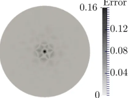
Concentration of the error around the singularity. First, we present one of the computations which drew our attention to the fact that the convergence could be better far from the singularity. For this example, we define Ω as the unit disk,
Ω“ tx “ px1, x2q P R2 :}x}2ă 1u,
Ω0 as the portion of Ω
Ω0 “ tx “ px1, x2q P R2 : 0.2ă }x}2ă 1u,
and finally x0 “ p0, 0q the origin. In this case, the exact solution uδ of problem pPδq is given by
upxq “ ´ 1 4π log ´ x21` x 2 2 ¯ .
When problempPδq is solved by the P1-finite element method, the numerical solution uhδ
con-verges to the exact solution uδ with order 1 in the L2-norm on the entire domain Ω (see [25]). This
example shows that the convergence far from the singularity is faster, since the order of convergence in this case is 2 (see [19]). The difference between the convergence rates for the L2
-norms on Ω and Ω0, led us to make the conjecture that the preponderant part of the error is concentrated around
the singularity, as can be seen in Figures 4,5,6, and7, which show the distribution of the error for 1{h » 10, 15, 20 and 30. Error 0.16 0.12 0.08 0.04 0
Figure 4: Error for 1{h » 10.
Error 0.16 0.12 0.08 0.04 0
Error 0.16 0.12 0.08 0.04 0
Figure 6: Error for 1{h » 20.
Error 0.16 0.12 0.08 0.04 0
Figure 7: Error for 1{h » 30.
Estimated orders of convergence. Figure 8 shows the estimated order of convergence for the H1
pΩ0q-norm for the Pk-finite element method, where k “ 1, 2, 3 and 4, in dimension 2. The
convergence far from the singularity (i.e. excluding a neighborhood of the point x0) is the same as
in the regular case: the Pk-finite element method converges at the order k on Ω0 for the H1-norm,
as proved in this paper with aa| lnphq| multiplier.
Elements P1 Elements P2 Elements P3 Elements P4 Order = 1.00 Order = 2.00 Order = 3.03 Order = 4.22 1 10´3 10´6 10´9 10´12 10´2 10´1
Figure 8: Estimated order of convergence for H1
pΩ0q-norm for the finite element method Pk, k “
6
Discussion
6.1 The three-dimensional case
Dirac mass. The approach presented in this paper can be extended to the three-dimensional case but straighforward adaptations of the proofs lead to a suboptimal result. In the case of Theorem1, the solution uδ belongs to W
1,p
0 pΩq for all p in r1, 3{2r. As a consequence the couple pp, p1q defined
in (14) has to be taken near from p3{2, 3q. For instance, p“ 3
2` ε and p
1
“ 1 3 ´ ε, so that, with the same notations, the result of Corollary 1 becomes
}uδ´ uhδ}´k`1,Ωď Chkh´ε´1{2|uδ´ uhδ|1,p,Ω.
Moreover, the discrete inf-sup condition in dimension 3 is
inf uhPVk h sup vhPVk h ş Ω∇uh¨ ∇vh }uh}1,p,Ω}vh}1,p1,Ω ě Ch ε`1{2.
Thus when dealing with the estimaye for |uδ´ uhδ|1,p,Ω, we get
|uδ´ uhδ|1,p,Ωď Ch´ε´1{2|uδ|1,p,Ω.
Finally, with the asymptotics in 3d
}uδ}1,p,Ω„ 1 3 ? 4π 1 3 ? 3´ 2p2, we get the estimate
}uδ´ uhδ}1,Ω0 ď CpΩ0,Ω1,Ωqhk´1 3
a | ln h|2. which is clearly suboptimal.
Theorem 3 is also suboptimal in 3d, even if better. Indeed, in 2d or in 3d, the proof readily adapts until the computation of }fε}0,Ω, which is in 3d
}fε}0,Ω“ 1 2 c 3 π 1 ε?ε, so that we get }uδ´ uhδ}1,Ω0 ď C ? h.
Line Dirac along a curve. In 3-dimension, a line Dirac δΓ along a curve Γ ĂĂ Ω belongs to
H´1´η for all ηą 0, so that the solution uΓ of the Poisson Problem with the line Dirac δΓ belongs
to H1´η. Actually, we have u
Γ P W1,ppΩq for all p P r1, 2r. In this case, with the same notations
and assumptions as in Theorem1, we have the following estimate for uΓand its Galerkin projection
uhΓ,
}uΓ´ uhΓ}1,Ω0 ď CpΩ0,Ω1,Ωqhk
a | ln h|,
which is quasi-optimal. This result is shown using the same arguments as the ones presented in Section 3, but cannot be obtained with the tools given in the proof detailed in [19].
6.2 Dirac mass near the boundary
Theorem 3 excludes some critical cases: Dirac mass should not be closer and closer to the border of the domain Ω. Indeed, for example in the case dpx0,BΩq „ h2, Assumption4 cannot be satisfied
with ε„ h{10, but only with ε „ h2
{10. Nevertheless, this small value of ε implies }u ´ uh}1,Ω0 ď C,
so that our method does not even prove the convergence of the approximate solution in this case. Actually, if the distance dpx0,BΩq tends to 0, the norm }u}1,p,Ω, for a fixed 1ď p ă 2, tends to `8,
so that the problem becomes more and more singular. But this question is a completely different problem and should be treated in a different way.
References
[1] J. P. Agnelli, E. M. Garau, and P. Morin. A posteriori error estimates for elliptic problems with Dirac measure terms in weighted spaces. ESAIM Math. Model. Numer. Anal., 48(6):1557–1581, 2014.
[2] T. Apel, O. Benedix, D. Sirch, and B. Vexler. A priori mesh grading for an elliptic problem with Dirac right-hand side. SIAM J. Numer. Anal., 49(3):992–1005, 2011.
[3] R. Araya, E. Behrens, and R. Rodr´ıguez. A posteriori error estimates for elliptic problems with Dirac delta source terms. Numer. Math., 105(2):193–216, 2006.
[4] I. Babuˇska. Error-bounds for finite element method. Numer. Math., 16:322–333, 1970/1971. [5] S. Bertoluzza. The discrete commutator property of approximation spaces. C. R. Acad. Sci.
Paris S´er. I Math., 329(12):1097–1102, 1999.
[6] H. Brezis. Analyse fonctionnelle. Collection Math´ematiques Appliqu´ees pour la Maˆıtrise. [Collection of Applied Mathematics for the Master’s Degree]. Masson, Paris, 1983. Th´eorie et applications. [Theory and applications].
[7] E. Casas. L2
estimates for the finite element method for the Dirichlet problem with singular data. Numer. Math., 47(4):627–632, 1985.
[8] E. Casas. Control of an elliptic problem with pointwise state constraints. SIAM J. Control Optim., 24(6):1309–1318, 1986.
[9] E. Casas, C. Clason, and K. Kunisch. Parabolic control problems in measure spaces with sparse solutions. SIAM J. Control Optim., 51(1):28–63, 2013.
[10] E. Casas and E. Zuazua. Spike controls for elliptic and parabolic PDEs. Systems Control Lett., 62(4):311–318, 2013.
[11] P. G. Ciarlet. The finite element method for elliptic problems, volume 40 of Classics in Applied Mathematics. Society for Industrial and Applied Mathematics (SIAM), Philadelphia, PA, 2002. Reprint of the 1978 original [North-Holland, Amsterdam; MR0520174 (58 #25001)].
[12] C. D’Angelo. Finite element approximation of elliptic problems with Dirac measure terms in weighted spaces: applications to one- and three-dimensional coupled problems. SIAM J. Numer. Anal., 50(1):194–215, 2012.
[13] K. Eriksson. Finite element methods of optimal order for problems with singular data. Math. Comp., 44(170):345–360, 1985.
[14] K. Eriksson. Improved accuracy by adapted mesh-refinements in the finite element method. Math. Comp., 44(170):321–343, 1985.
[15] G. R. Fulford and J. R. Blake. Muco-ciliary transport in the lung. J. Theor. Biol., 121(4):381– 402, 1986.
[16] P. Grisvard. Elliptic problems in nonsmooth domains, volume 24 of Monographs and Studies in Mathematics. Pitman (Advanced Publishing Program), Boston, MA, 1985.
[17] J. D. Jackson. Classical electrodynamics. John Wiley & Sons, Inc., New York-London-Sydney, second edition, 1975.
[18] D. Jerison and C. E. Kenig. The inhomogeneous Dirichlet problem in Lipschitz domains. J. Funct. Anal., 130(1):161–219, 1995.
[19] T. K¨oppl and B. Wohlmuth. Optimal a priori error estimates for an elliptic problem with Dirac right-hand side. SIAM J. Numer. Anal., 52(4):1753–1769, 2014.
[20] L. Lacouture. A numerical method to solve the Stokes problem with a punctual force in source term. C. R. Mecanique, 343(3):187–191, 2015.
[21] D. Leykekhman, D. Meidner, and B. Vexler. Optimal error estimates for finite element dis-cretization of elliptic optimal control problems with finitely many pointwise state constraints. Comput. Optim. Appl., 55(3):769–802, 2013.
[22] J. A. Nitsche and A. H. Schatz. Interior estimates for Ritz-Galerkin methods. Math. Comp., 28:937–958, 1974.
[23] R. Rannacher and B. Vexler. A priori error estimates for the finite element discretization of elliptic parameter identification problems with pointwise measurements. SIAM J. Control Optim., 44(5):1844–1863, 2005.
[24] A. H. Schatz and L. B. Wahlbin. Maximum norm estimates in the finite element method on plane polygonal domains. II. Refinements. Math. Comp., 33(146):465–492, 1979.
[25] L. R. Scott. Finite element convergence for singular data. Numer. Math., 21:317–327, 1973/74. [26] L. R. Scott and S. Zhang. Finite element interpolation of nonsmooth functions satisfying
boundary conditions. Math. Comp., 54(190):483–493, 1990.
[27] L. B. Wahlbin. Local behavior in finite element methods. In Handbook of numerical analysis, Vol. II, Handb. Numer. Anal., II, pages 353–522. North-Holland, Amsterdam, 1991.
[28] L. B. Wahlbin. Superconvergence in Galerkin finite element methods, volume 1605 of Lecture Notes in Mathematics. Springer-Verlag, Berlin, 1995.