HAL Id: hal-01352802
https://hal.inria.fr/hal-01352802
Submitted on 9 Aug 2016
HAL is a multi-disciplinary open access
archive for the deposit and dissemination of
sci-entific research documents, whether they are
pub-lished or not. The documents may come from
teaching and research institutions in France or
abroad, or from public or private research centers.
L’archive ouverte pluridisciplinaire HAL, est
destinée au dépôt et à la diffusion de documents
scientifiques de niveau recherche, publiés ou non,
émanant des établissements d’enseignement et de
recherche français ou étrangers, des laboratoires
publics ou privés.
Point Cloud Library: A study of different features part
of the Point Cloud Library
Salman Maqbool, Umar Ghaffar
To cite this version:
Salman Maqbool, Umar Ghaffar. Point Cloud Library: A study of different features part of the Point
Cloud Library. [University works] National University of Sciences and Technology (NUST). 2016.
�hal-01352802�
Point Cloud Library
A study of different features part of the Point Cloud Library
Salman Maqbool, Umar Ghaffar
Department of Robotics and Intelligent Machines Engineering SMME, NUST
Islamabad, Pakistan
{salmanmaq, umarghaffar30}@gmail.com
Abstract — Point Cloud Library (PCL) is an open
source library, written in C++, for 3D point cloud processing. It was published by Rusu et al after his PhD dissertation and his work at Willow Garage. It’s the epitome of 3D computer vision nowadays, and has numerous academic and industrial applications. This paper describes our work in the Point Cloud Library.
Keywords—Point Cloud Library, Point Cloud, 3D Computer Vision
I. INTRODUCTION
Point Cloud Library is a library of robust tools for point cloud manipulation. With the advent of low price 3D cameras like Kinect, RealSense etc, usage of depth information in Computer Vision applications has grown. Point Cloud Library incorporates a variety of algorithms for a number of computer vision applications including feature extraction, segmentation, object detection, recognition, and classification, point cloud registration, and pose estimation.
We studied different algorithms part of the Point Cloud Library. Our primary intuition was to follow the comprehensive tutorials listed on Point Cloud Library’s website [1]. We describe the algorithms we implemented which are part of the PCL 1.7 in the rest of the paper. Our implementations were in Ubuntu 14.04 LTS environment set up in a virtual environment.
II. THEPCDFILEFORMAT
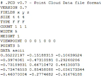
The PCL uses a specific file format to store and read point cloud data and other information pertaining to the point cloud dataset. The specific file format is the Point Cloud Document (.pcd) format. It uses the PCD IO and the Point Types libraries to read/write and specify the data contained in the PCD files respectively. Figure 1 shows a sample PCD file and its contents. As we can see, it contains X, Y, and Z coordinates for each point in the point cloud. It also shows a hoard of other useful information which is later used in feature extraction especially the viewpoint direction component which is used to estimate very useful features from images, some of which we will see in the coming sections.
Figure 1: PCD File showing the X, Y, Z point data
We can also transform a point cloud dataset using the Transformation matrix containing the rotation and the translation components. Figure 2 shows one such transformation obtained through a rotation of p/4 radians
about the z-axis, and a translation of 2.5 m along the x-axis. The following transformation matrix was defined:
Figure 2: Transformation of a point cloud dataset. The original point cloud, showing a mug placed on a table, is shown in white. The transformed point cloud is shown in red.
III. NORMALESTIMATION
The very first features which we extract from a given dataset are the surface normals. There are two prominent methods for the task:
Obtain the underlying surface from the acquired point cloud dataset, using surface meshing techniques, and computing the surface normals from the mesh.
Approximate the surface normals from the point cloud dataset directly
We followed the tutorial given on the PCL website. The theoretical primer is as described:
For each point, Pi, the covariance matrix is obtained as:
-where k is the defined number of nearest neighbors or the number of nearest neighbors in a search radius r
- represents the centroid of the nearest neighbors - is the j-th eigen-value
- is the j-th eigen-vector
Estimating normal to a point on the surface is approximated by the problem of estimating the normal of a plane tangent to the surface, which in turn becomes a least-square plane fitting estimation problem. The outputs are the normal in X direction, in the Y direction, and the Z direction, and the curvature at that point, where the curvature is estimated as:
Figure 3 shows the starting few lines of the PCD dataset we used to estimate the surface normals and the associated surface normals obtained using the estimation algorithm.
Figure 3: The X, Y, Z, X-normal, Y-normal, Z-normal, and curvature obtained using the normal estimation algorithm.
Figure 4 visualizes the point cloud dataset used, and Figure 5 visualizes the estimated surface normals.
Figure 4: Visualization of the Point Cloud dataset in the PCL viewer. The scene shows a mug on a table top.
Figure 5: Visualization of the estimated surface normals for the scene shown in Figure 4 and the associated PCD dataset shown in Figure 3.
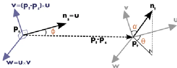
IV. POINTFEATUREHISTOGRAMS (PFH)[2] Point Feature Histograms are another set of feature descriptors which are invariant to the pose of the surface, and present much more information about the surface than the surface normals, which may have similar values over the range of the point cloud. The following diagram shows the estimated surface normals and the calculated Point Feature Histogram parameters for a point cloud pair:
Figure 6: Point Feature Histogram (PFH) descriptors
After we have estimated the surface normals ns and nt for the
pair, we assign frames as follows:
After the frame assignment, we calculate the PFH descriptors as the difference between the two normals, for each pair of normals as:
Where are the set of PFH descriptors for a pair of points. The descriptors for each query point are binned into a histogram to obtain the PFH features for a given point cloud. Figure 7 shows one such histogram.
Figure 7: Point Feature Histogram descriptors
We obtained the Point Feature Histograms for a simple point cloud given in Figure 8. A subset of the PFH descriptors for 13 of the points are given in Figure 9.
Figure 8: Sample dataset used for calculating the PFH, FPFH, and the VFH features
The PFH features calculation is a really slow process though, with a runtime of O (nk2). We tried to calculate the PFH descriptors for a dataset containing 209280 points. We ran the algorithm on a 2nd generation Intel core i5 machine with 4 GB of RAM, and it wasn’t able to complete the computation even after an hour. That’s why we need a better set of features more suitable for real world, real time applications. We introduce such features in the next section.
Figure 9: A subset of the PFH features for 13 points of the point cloud shown in Figure 8
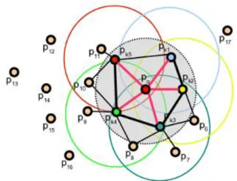
V. FASTPOINTFEATUREHISTOGRAMS(FPFH)[3] Fast Point Feature Histograms are a simplification of the Point Feature Histograms described in the previous section. The simplification results from the fact that while calculating the nearest neighbors for the point cloud, a neighbor of one point will also be a neighbor of another point in the search radius. These relationships are cached and hence are not computed for each point. Figure 10 highlights this relationship. This leads to a runtime of O (nk), a drastic reduction from PFHs.
Figure 10: Relationship between nearest neighbors on a
query point pq and its nearest neighbors. Such a
relationship is useful when calculating FPFH features and speeds up the feature extraction process.
After the surface normals have been obtained, and the PFH descriptors <α,Φ,Θ> computed, the FPFH descriptors are computed as:
where ωk is the factor by which we weigh the Simple PFH
(SPFH) descriptors for nearest neighbor pk. In our study, ωk
represents the distance between a query point pq and its nearest
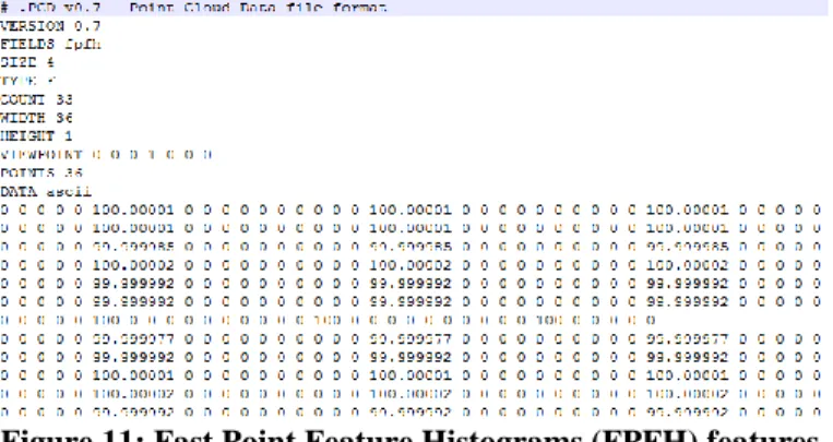
neighbor pk. We obtained the FPFH features for the point
cloud shown in Figure 8, and sample results are shown in Figure 11 below.
Figure 11: Fast Point Feature Histograms (FPFH) features for the point cloud shown in Figure 8
VI. VIEWPOINTFEATUREHISTOGRAMS(VFH)[4]
Viewpoint Feature Histograms (VFH) are an extension of the Point Feature Histograms (PFH) described in section IV. The viewpoint direction component i.e. the vector from the viewpoint direction to the centroid of the input point cloud is used directly in the relative normal angle calculations. First, the centroid of the input point cloud is determined as:
The PFH descriptors are then computed as described earlier using the following relations:
The centroid and the PFH descriptors are shown in Figure 12.
Figure 12: Point cloud centroid and the PFH descriptors
The final viewpoint component is calculated as the angle β between the viewpoint vector Vp and the centroid normal as:
The angle β can be visualized in the figure below:
Figure 13: Visualization of the viewpoint feature descriptors
The histogram of the angles each normal makes with the viewpoint direction components is obtained. Such a histogram is shown in Figure 14.
Figure 14: Viewpoint Features Histogram (VFH) features
Viewpoint Feature Histograms (VFH) provide an efficient set of features for use in different applications including object detection, object recognition, object classification, as well as 6 DoF pose estimation.
Unlike PFH and FPFH, VFH is a single feature for the entire point cloud, and not features for individual points. We discuss cluster extraction and object segmentation in the next section, after which we will discuss point cloud cluster classification in PCL.
VII. CLUSTEREXTRACTION[5]
From a given point cloud, individual object clusters can be extracted, which results in significant reduction of the overall processing time. The algorithm utilizes kd-tree based nearest neighbor search to segment the point cloud into individual
point clouds based on the Euclidean distance. Figure 15 shows the clusters extracted from the point cloud shown earlier in Figure 2. Note that the clusters are extracted from the original point cloud, not the transformed one.
Figure 15: Euclidean cluster extraction of the point cloud shown in Figure 2
VIII. OBJECTCLASSIFICATIONUSINGVFH[5] Cluster extraction together with VFH features provides a powerful set of tools for object recognition and classification. Object classification in PCL is a two stage process:
i. Training Stage: Given a segmented object cluster, the VFH features are computed, stored, and a kd-tree built.
ii. Testing Stage: Given a point cloud, extract object clusters as discussed in Section VII. Then extract the VFH descriptors for each cluster, and use nearest neighbor search to search for objects in the trained kd-tree.
At dataset already provided at [6] is used, containing 290 objects, for which the VFH descriptors are pre-computed. The dataset contains objects containing a subset of the objects presented in Figure 16 and the point clouds presented in Figure 17.
Figure 16: Training data set
Figure 17: Point clouds for the training dataset
The algorithm was run for three different test cases and the figures below show the results. The query point cloud cluster is shown in the bottom left of each image, and its 15 nearest neighbors are shown accordingly. The numbers is each box represent the similarity measure of each cluster with respect to the query point cloud cluster.
Figure 18: Test case 1: Showing the original point cloud (bottom left) and its nearest neighbors from the dataset
Figure 20: Test case 3
IX. CONCLUSIONANDFUTUREWORK
As we can see, the results of the algorithm are remarkable and it successfully identified the object itself and other object clusters similar to it. In fact, the reported object recognition accuracy is as high as 98.52 % for a training set containing 55000 point clouds [4]. This also shows that the Point Cloud Library and its algorithms are scalable to large datasets. In addition to that, they work well with noisy data and the processing time is quite fast at 0.3 ms/cluster, making it ideal to use in real world applications.
Now that we have obtained the VFH signatures for different point clouds, we plan to use them with different machine learning algorithms in MatLab. In addition to that, we plan to obtain real world data using Kinect and use the algorithms presented above with that for robotic applications.
References
[1] www.pointclouds.org
[2] Rusu, Radu Bogdan, et al. "Aligning point cloud views using persistent feature histograms." Intelligent Robots
and Systems, 2008. IROS 2008. IEEE/RSJ International Conference on. IEEE, 2008.
[3] Rusu, Radu Bogdan, Nico Blodow, and Michael Beetz. "Fast point feature histograms (FPFH) for 3D registration." Robotics and Automation, 2009. ICRA'09.
IEEE International Conference on. IEEE, 2009.
[4] Rusu, Radu Bogdan, et al. "Fast 3D recognition and pose using the viewpoint feature histogram." Intelligent Robots
and Systems (IROS), 2010 IEEE/RSJ International Conference on. IEEE, 2010.
[5] Aldoma, Aitor, et al. “Point Cloud Library: Three-Dimensional Object Recognition and 6 DoF Pose Estimation” Robotics and Automation Magazine, 2012. IEEE, Sep 2012.
[6] www.pointclouds.org/documentation/tutorials/vfh_recogn ition.php