HAL Id: hal-02366686
https://hal.archives-ouvertes.fr/hal-02366686
Preprint submitted on 16 Nov 2019HAL is a multi-disciplinary open access
archive for the deposit and dissemination of sci-entific research documents, whether they are
pub-L’archive ouverte pluridisciplinaire HAL, est destinée au dépôt et à la diffusion de documents scientifiques de niveau recherche, publiés ou non,
Primordial black holes from the preheating instability
Jérôme Martin, Theodoros Papanikolaou, Vincent Vennin
To cite this version:
Jérôme Martin, Theodoros Papanikolaou, Vincent Vennin. Primordial black holes from the preheating instability. 2019. �hal-02366686�
Primordial black holes from the
preheating instability
J´
erˆ
ome Martin,
aTheodoros Papanikolaou,
bVincent Vennin
b,aaInstitut d’Astrophysique de Paris, UMR 7095-CNRS, Universit´e Pierre et Marie Curie, 98bis boulevard Arago, 75014 Paris, France
bLaboratoire Astroparticule et Cosmologie, Universit´e Denis Diderot Paris 7, 75013 Paris, France
E-mail: [email protected],[email protected],
Abstract.
After the end of inflation, the inflaton field oscillates around a local minimumof its potential and decays into ordinary matter. These oscillations trigger a resonant instability for cosmological perturbations with wavelengths that exit the Hubble radius close to the end of inflation. In this paper, we study the formation of Primordial Black Holes (PBHs) at these enhanced scales. We find that the production mechanism can be so efficient that PBHs subsequently dominate the content of the universe and reheating proceeds from their evaporation. Observational constraints on the PBH abundance also restrict the duration of the resonant instability phase, leading to tight limits on the reheating temperature that we derive. We conclude that the production of PBHs during reheating is a generic and inevitable property of the simplest inflationary models, and does not require any fine tuning of the inflationary potential.
Keywords:
physics of the early universe, primordial black holes, inflationContents
1 Introduction 1
2 Inflation and the preheating instability 3
3 PBH formation during reheating 8
3.1 Formation criterion 8
3.2 Refined formation criterion: Hawking evaporation 9
3.3 Mass fraction 10
3.4 Renormalising the mass fraction at the end of the instability 12
3.4.1 Renormalisation by inclusion 12
3.4.2 Renormalisation by premature ending 14
3.5 Evolving the mass fraction 14
3.6 Reheating through PBH evaporation 17
3.7 Planckian relics 20
4 Observational consequences 20
4.1 The onset of the radiation era 20
4.2 Constraints from the abundance of PBHs 22
4.3 Constraints from the abundance of Planckian relics 25
5 Discussion and conclusions 26
A Black holes formation from scalar field collapse 29
B Calculation of the critical density contrast 36
1
Introduction
The reheating stage [1–4] is a crucial part of the inflationary scenario [5–9]. It allows inflation to come to an end, and describes how the inflaton field decays and produces ordinary matter. Although reheating appears to be a rather complicated process, as far as the large scales probed by the Cosmic Microwave Background (CMB) anisotropies are concerned [10, 11], the influence of this epoch on the predictions of inflation is simple, at least in single-field models. This is due to the fact that, on large scales, the curvature perturbation is conserved [12, 13], which implies that the details of the reheating process do not a↵ect the inflationary predictions. In fact, those predictions are sensitive to a single parameter, the so-called reheating parameter [14], which is a combination of the reheating temperature and of the mean equation-of-state parameter, and which determines the location of the observational window along the inflationary potential. Given the restrictions on the shape of the potential now available [15–19], this can be used to constrain reheating [20–23].
On small scales however, the situation is di↵erent. It was indeed shown in Ref. [24] (see also Ref. [25]) that, for scales leaving the Hubble radius during the last⇠ 10 e-folds of inflation (if the energy scale of inflation is not tuned to extremely low values), there is a parametric instability that can lead to an enormous growth of perturbations. This can cause early structure formation and/or gravitational waves production [24–26], and may open a new observational window on inflation and reheating.
In the present paper, we study yet another possible consequence of the presence of this instability, namely the production of Primordial Black Holes (PBHs) [27, 28]. The motivation is twofold. First, this may lead to a new inflationary mechanism for black hole production which is completely natural and generic. Usually, it is necessary to consider very specific potentials in order for this production to be efficient. In this work, the only assumption is that the potential can be approximated by a parabola around its minimum. Except for fine-tuned situations (where, for instance, a symmetry prevents the presence of a quadratic term in the Taylor expansion of the potential about its minimum), this is always the case. Second, tight constraints on the abundance of PBHs have been placed in various mass ranges (for a review, see e.g. Refs. [29,30]), and this can be used to obtain extra information about the reheating epoch.
The paper is organised as follows. In the next section, Sec. 2, we briefly review Ref. [24] and the physical mechanism that leads to the instability mentioned above. Then, in Sec.3, we study under which physical conditions PBHs are formed. In Sec.3.1, based on Ref. [31], we derive the critical density contrast from the requirement that the instability must last long enough, before reheating is completed, to allow the initial scalar field overdensity to form a black hole. In Sec.3.2, the corresponding criterion is refined by taking Hawking evaporation into account. We then calculate the mass fraction at the end of the instability phase in Sec.3.3. Due to the high efficiency of the instability, we find that the corresponding values for the fraction of the universe comprised in PBHs can be larger than one, which is not possible. The mass fraction must therefore be renormalised, which is done in Sec.3.4. We propose two ways to carry out this procedure, one which accounts for the possible inclusion of PBHs within larger ones (Sec.3.4.1), and one which accounts for the premature termination of the instability phase by the backreaction
of PBHs (Sec. 3.4.2). Having calculated the abundance of PBHs at the end of the
instability, in Sec.3.5, we proceed with calculating their abundance in the subsequent radiation-dominated epoch. In some cases, we find that PBHs are so abundant that the radiation-dominated era is delayed and we discuss under which conditions this occurs in Sec.3.6. In Sec.3.7, we also consider the case where black holes do not entirely evaporate but leave Planckian relics behind. In Sec.4, we derive the observational consequences of the above-described mechanism. In Sec.4.1, we establish restrictions on the energy density at the onset of the radiation dominated era (the reheating temperature). From current constraints on PBHs (Sec. 4.2) and Planckian relics (Sec. 4.3) abundances, we then derive constraints on the energy scale of inflation and the reheating temperature. In Sec. 5, we summarise our main results and present our conclusions. Finally, the paper ends with two appendices. In AppendixA, we explain how a scalar field (here, the inflaton field) can collapse and form a black hole and, in AppendixB, we use these
considerations to derive the expression of the critical density contrast used in the rest of the paper.
2
Inflation and the preheating instability
We consider scenarios where inflation is realised by a single scalar field (the inflaton), which slowly rolls down its potential V ( ) and then oscillates at the bottom of it. In flat Friedmann-Lemaˆıtre-Robertson-Walker space-times, the dynamics of the homogeneous inflaton field is driven by the Klein-Gordon and the Friedmann equations,
¨ + 3H ˙ + V0( ) = 0 , H2 = V ( ) + ˙2 2 3MPl
. (2.1)
Hereafter, H = ˙a/a is the Hubble parameter, a(t) is the scale factor, a dot denotes derivative with respect to cosmic time, and MPl is the reduced Planck mass. These
equations can be solved numerically or with the help of the slow-roll approximation, and the solution is insensitive to the choice of initial conditions due to the presence of the slow-roll attractor [32–36]. Inflation ends when the first slow-roll parameter ✏1⌘ H/H˙ 2 reaches one; then, starts the reheating/preheating phase.
Close to its minimum, we assume the potential to be approximated by a quadratic function,1
V ( ) = m
2 2
2. (2.2)
When, after the end of inflation, the inflaton field explores this part of the potential,
H⌧ m and behaves as
(t)' 0⇣a0 a
⌘3/2
sin (mt) . (2.3)
This implies that the energy density stored in redshifts on average as matter [1], ⇢ / a 3, and that the oscillations have a frequency given by the mass m. Here, the subscript “0” just denotes a reference time that might be taken at the end of inflation. Let us stress that we only assume the inflationary potential to be of the quadratic form towards the end of inflation, see footnote1. No restriction on its shape is imposed at the scales where the cosmological perturbations observed in the CMB are produced, where the potential can e.g. be of the plateau type, and provide a good fit to observations. This means that the parameter m in Eq. (2.2) should not be fixed to match the CMB power spectrum amplitude as usually done, but should be left free in order to scan di↵erent values of Hend, namely di↵erent energy scales at the end of inflation. In practice, this can be done
1As the amplitude of the oscillations get damped, the leading order in a Taylor expansion of the
function V ( ) around its minimum quickly dominates, which is of quadratic order unless there is an exact cancellation at that order. The validity of this approximation is further discussed below.
as follows. Inflation ends when2 end' 1.0092MPl. Given that ✏1 = 3 ˙2/2/(V + ˙2/2), at the end of inflation, ˙2= V , and one can relate H
end to m according to m = 2HendMPl
end. (2.5)
In this way, by varying m one can vary the value of the Hubble parameter at the end of inflation, Hend.
For the cosmological perturbations, there is a single gauge-invariant scalar degree of freedom that can be described with the Mukhanov-Sasaki variable [12, 13] v, which is a combination of the perturbed inflaton field and of the Bardeen potential, the latter being a generalisation of the gravitational Newtonian potential [37]. Its Fourrier component vk evolves according to [38] v00k+ ✓ k2 z 00 z ◆ vk = 0, (2.6)
where a prime denotes a derivative with respect to conformal time ⌘, defined as dt = ad⌘. In this expression, z⌘p2✏1aMPl and is such that
z00 z = a 2H2h⇣1 + ✏2 2 ⌘ ⇣ 2 ✏1+ ✏2 2 ⌘ + ✏2✏3 2 i , (2.7)
where ✏2⌘ d ln ✏1/dN and ✏3⌘ d ln ✏2/dN are the second and the third slow-roll param-eters respectively. The initial condition is taken in the Bunch-Davies vacuum, i.e. such that vk ! e ik⌘/
p
2k when k aH, and the function z00/z is evaluated on the back-ground dynamics that has been numerically integrated as explained above. In this way, one can compute the amplitude of vk at the end of inflation for each mode k.
It is convenient to introduce the curvature perturbation ⇣ defined as ⇣ = v/z since this quantity is conserved on super-Hubble scales, and to compute the power spectrum P⇣ = k3|⇣k|2/(2⇡2) of that quantity at the end of inflation. It is displayed in Fig.1for the value of m corresponding to ⇢inf ⌘ 3Hend2 MPl2 = 10
12M4
Pl ' 2.43 ⇥ 10
15GeV 4, as
a function of k/kend, where kend= aendHendis the scale that exits the Hubble radius at the end of inflation, see also Fig.2. The blue solid line corresponds to the numerical solution of Eq. (2.6), while the black dashed line stands for the slow-roll approximated
2The value obtained for
endis independent of the mass parameter m, which can be seen with writing
Eqs. (2.1) as a single equation for in terms of the number of e-folds N = ln a,
d2 dN + " 3 1 2M2 Pl ✓ d dN ◆2# ✓d dN + M 2 Pl V0 V ◆ = 0 . (2.4)
In this equation, the potential only appears through the combination V0/V , in which the mass parameter
m cancels out. Since the first slow-roll parameter can be written as ✏1 = (d /dN )2/(2MPl2), the value
10 20 10 16 10 12 10 8 10 4 100
k/k
end 10 15 10 14 10 13 10 12 10 11 10 10 10 9P
⇣ ,end numerical slow rollFigure 1. Power spectrum of the curvature perturbation at the end of inflation for m ' 1.14⇥ 10 6M
Pl, corresponding to ⇢inf ⌘ 3Hend2 MPl2 = 10 12M4
Pl ' 2.43 ⇥ 10
15GeV 4, as a
function of k/kend, where kend is the scale that exits the Hubble radius at the end of inflation.
The blue solid line corresponds to the numerical solution of Eq. (2.6) while the black dashed line stands for the slow-roll approximation (2.8).
solution of that equation, namely [39,40]
P⇣,end= 8 > > > > < > > > > : H2 ⇤(k) 8⇡2M2 Pl✏1⇤(k) " 1 + ✓ k kend ◆2# [1 2 (C + 1) ✏1⇤(k) C✏2⇤(k)] if k < kend Hend2 8⇡2M2 Pl " 1 + ✓ k kend ◆2# if k > kend . (2.8) In this expression, for the modes that cross out the Hubble radius before the end of inflation, k < kend, the functions H⇤(k), ✏1⇤(k) and ✏2⇤(k) respectively denote the values of H, ✏1and ✏2at the time when the mode k exits the Hubble radius, and are evaluated in the numerical solution of Eqs. (2.1). The parameter C ' 0.7296 is a numerical constant. One can check in Fig.1that, except for the very few modes that are close to the Hubble scale at the end of inflation and for which the amount of power is underestimated, Eq. (2.8) provides a very good fit to the numerical solution.
As already mentioned, after the end of inflation, the inflaton oscillates at the bot-tom of its quadratic potential and the evolution of the perturbations through this epoch strongly depends on the scales considered. On large scales (for instance, CMB scales), the conservation of curvature perturbation is sufficient to establish that the power
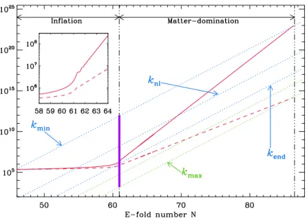
spec-Figure 2. Evolution of the relevant physical scales versus the e-folds number. The continuous red line denotes the Hubble radius, which is also the upper bound of the instability band, while the dashed red line represents the scalep3Hm which corresponds to the lower bound of the resonance band. The dotted lines represent the physical wavelengths of di↵erent Fourier modes: the “green modes” enter the instability mode from below while the “blue modes” enter it from above. The inset shows the detailed behaviours of the Hubble radius andp3Hm at the transition between inflation and reheating. Figure taken from Ref. [24].
trum (2.8) calculated at the end of inflation propagates through the reheating epoch without being distorted. However, on smalle scales, things can be very di↵erent. As shown in Ref. [24], for modes satisfying
aH < k < ap3Hm , (2.9)
see Fig. 2, the oscillations source a parametric resonance (in the narrow resonance regime). The reason is that, thanks to these oscillations, Eq. (2.6) becomes a Math-ieu equation and the condition (2.9) is in fact equivalent to being in the first instability band of that equation. We see that the instability occurs if the physical wavelength of a mode is smaller than the Hubble radius (continuous red line in Fig.2) during reheating and larger than a new scale given by p3Hm (dashed red line in Fig. 2). Moreover, two types of mode can be distinguished. The “blue modes” in Fig.2 exit the Hubble radius during inflation and re-enter it during reheating; these modes therefore enter the instability band from above. On the other hand, the “green modes” never exit the Hub-ble radius and enter the instability band from below by crossing the new scalep3Hm . Once within the instability band, as described in Ref. [24], the fluctuations get strongly
amplified, such that the density contrast grows linearly with the scale factor. E↵ectively, they thus behave as pressureless matter perturbations in a pressureless matter universe. In what follows, this epoch is referred to as the “instability phase”. As explained in Sec. 1, during this epoch, cosmological perturbations at the amplified scales may col-lapse into PBHs. When the inflaton decays into other degrees of freedom (or when the PBHs take the inflaton over, see below), the instability stops, and the density of black holes evolves under various physical e↵ects (cosmic expansion, Hawking evaporation, accretion, merging, etc.).
Let us further discuss the quadratic approximation for the inflationary potential. The largest scales amenable to parametric resonance during the instability phase are such that k = ainstabHinstab, where the time tinstab denotes the end of the instability phase (the corresponding Fourier mode is denoted “kmin” in Fig. 2). During infla-tion, they cross out the Hubble radius at a number of e-folds ⇠ ln(Hend/Hinstab)/3 before the end of inflation, where we recall that Hend is the value of the Hubble pa-rameter at the end of inflation and where we have used that, during the instabil-ity, the universe is matter dominated at the background level. Since observational bounds on the tensor-to-scalar ratio impose [11] Hend < 8⇥ 1013GeV, and given that
Hinstab> HBBN ⇠ (10 MeV)2/
p
3MPl2 ⇠ 10 23GeV, where hereafter “BBN” stands for
big-bang nucleosynthesis, this number of e-folds needs to be smaller than⇠ 28.3 All the scales of interest for the problem at hand are therefore generated in the last 28 e-folds of inflation, where we assume the potential to be well approximated by the quadratic form (2.2). Although one may be suspicious that this approximation holds for 28 e-folds, let us stress that this value is in fact an extreme upper bound that comes from satu-rating the condition Hinstab > HBBN, while we will see below that most of the relevant parameter space is such that Hinstab and HBBN are separated by many orders of magni-tude and this number of e-folds is in fact much smaller. In practice, potentials favoured by the data (such as plateau ones) tend to be shallower than the quadratic one away from the end of inflation, and we have explicitly checked that this approximation only slightly underestimates the amplitude of scalar perturbations in such potentials, leading to conservative statements regarding the amount of PBHs.4 It is nonetheless clear that the calculational program laid out below can easily be performed for any given poten-tial, such that the approximation (2.2) for the last e-folds of inflation is released. In this work, it however allows us to carry out a full parameter-space analysis, where the energy scale of inflation can be varied without relying on a specific potential. We will see that this provides an overall picture where several interesting regions are identified, in which
3Strictly speaking the tensor-to-scalar ratio r is related to H
⇤, the energy scale of inflation at the
time the CMB modes left the Hubble radius during inflation, which is a di↵erent quantity that Hend, the
energy scale at the end of inflation. Here, we neglect the di↵erence between those two quantities. This approximation is especially accurate for plateau models, namely for the models favoured by the most recent astrophysical data.
4Hereafter, “conservative” refers to the fact that the approximations performed in this work tend
to underestimate the amount of PBHs, such that our results can be viewed as lower bounds on their abundance, and the regions of parameter space that are excluded because they produce too many PBHs might extend beyond what is obtained below.
a more detailed analysis can always be carried out.
3
PBH formation during reheating
We have just seen that the modes in the resonance band (2.9) behave as pressureless mat-ter fluctuations in a pressureless matmat-ter universe. In Ref. [31] and in the two appendices, see Eq. (B.7), it is shown that they collapse into PBHs after a time [31]5
tcollapse= ⇡
H [tbc(k)] k3/2[tbc(k)]
, (3.1)
where tbc(k) denotes the “band-crossing” time, i.e. the time at which the mode k crosses in the instability band (2.9).
Let us note that, in a matter-dominated universe, aH decreases as a 1/2 while apH increases as a1/4, so the bounds defining the instability band (2.9) are such that, when a mode crosses in the band, it remains in the band (in other words, modes cannot cross out the band).
This instability stops when the coherent oscillations of the inflaton are over. This can happen e.g. when the inflaton decays into other fields. In the case of perturbative preheating, this occurs when the Hubble parameter drops below the decay rate of the inflaton, and for this reason, hereafter this time is referred to as t . One should however note that the results derived below are independent of the precise way in which the phase of coherent oscillations stop, since the time at which this happens (regardless of the way it happens) is simply one of the parameters in the present scenario.6
Let us also stress that, for later convenience, we have introduced the two notations
tinstab and t . As mentioned above, tinstab denotes the end of the instability while t
denotes the time at which the field decays. Although they are identical in the standard picture, we will see below that there are cases where they di↵er (for instance if PBHs come to dominate the universe content before the inflaton decays), which explains the need for two distinct notations.
3.1 Formation criterion
Let us now determine under which conditions PBHs form. The last mode to enter the band (2.9) “from above” is such that k = a H , which leads to k/kend = (⇢ /⇢inf)1/6. The last mode that enters the band “from below” is, on the other hand, such that k = a p3H m . In this paper, however, we restrict ourselves to modes that enter the instability band from above. Indeed, as already noticed, the modes that enter the mode from below have never crossed out the Hubble radius and their status is unclear: in practice, one should derive the full real-space profile of the over-densities produced by
5Here, we correct an error of a factor 2 in Eq. (84) of Ref. [31].
6As one approaches the point where H ⇠ , the averaged background equation-of-state parameter
becomes progressively finite and this could lead to shutting o↵ the instability before the time of
pertur-bative decay [41]. In this case H > , but again, H is simply used as a parameter to describe the time
the instability band [42], which is beyond the scope of the present work. We therefore restrict our analysis to a subset of the instability band (2.9) only, namely to modes such that ✓ ⇢ ⇢inf ◆1/6 < k kend < 1 . (3.2)
Obviously, the incorporation of the modes that enter the instability band “from below” could lead to further PBHs production, and the results presented below are therefore conservative in the sense of footnote4.
Let us now determine under which condition the time spent in the instability band (2.9) is enough for PBHs to form. Since the background energy density decays as pressureless matter during the instability, one has
t tbc= 2 3Hbc "✓ a abc ◆3/2 1 # . (3.3)
Requiring that this is larger than the time (3.1) required for PBHs to form, one obtains the following condition,
✓ 3⇡ 2 ◆2/3"✓ k kend ◆3r ⇢inf ⇢ 1 # 2/3 < k[tbc(k)] < 1 , (3.4) where the upper bound comes from the requirement that PBHs form in the perturbative regime (the enforcement of this condition is again conservative with regards to the PBH abundance).
3.2 Refined formation criterion: Hawking evaporation
The mass M of the PBH associated to the scale k is given by some fraction ⇠ of the mass contained within a Hubble radius at the time tbc when k re-enters the Hubble radius. Making use of the fact that the background energy density decays as pressureless matter during the instability, one obtains
M (k) = ⇠ 3M 2 Pl 3/2 p⇢ inf ✓ k kend ◆ 3 . (3.5)
These masses are typically very small and can be such that they disappear by Hawking evaporation before the end of the instability. Since the evaporated black holes should be removed from the mass fraction, let us determine under which conditions this happens. The time of evaporation of a black hole with mass M is given by [43]
tevap(M ) =10240 g M3 M4 Pl , (3.6)
where g is the e↵ective number of degrees of freedom. For the black hole to survive until the end of the instability, one should therefore check that tevap> t tcollapse =
t tbc (tcollapse tbc), where t tbc is given in Eq. (3.3) and tcollapse tbc is given in Eq. (3.1). This imposes the condition
k[tbc(k)] < " 2 3⇡ ✓ k kend ◆3r ⇢inf ⇢ 2 3⇡ 10240 g ⇠3 ⇡ (3MPl) 4 ⇢inf ✓ k kend ◆ 6# 2/3 . (3.7)
When the quantity inside the square brackets is negative, Hawking evaporation cannot proceed before the end of the instability phase and this does not need to be taken into account. Otherwise, the value for max(k) now needs to be taken as the minimum value between the right-hand side of Eq. (3.4) and the right-hand side of Eq. (3.7). Let us note that, comparing Eqs. (3.4) and (3.7), one always has max(k) > c(k), unless c > 1, in which case we simply take the mass fraction to vanish.
3.3 Mass fraction
Assuming Gaussian statistics P for the density contrast perturbation at the band-crossing time, with a variance given by the power spectrum P , the mass fraction of PBHs can be expressed as [44] (M, t )⌘ d⌦PBH(k, t ) d ln M = 2 Z max(k) c(k) P ( )d = erfc " c(k) p 2P (k) # erfc " max(k) p 2P (k) # , (3.8) where erfc is the complementary error function and we have followed the usual Press-Schechter practice of multiplying by a factor 2. In this expression, we recall that M and k are related through Eq. (3.5), that the minimum value of the density contrast, c(k), is given by the left-hand side of Eq. (3.4), and that the maximum value, max(k), is given by the considerations presented in Sec. 3.2. On the other hand P (k) [where the argument tbc(k) has been dropped for notational convenience] can be obtained from the following considerations. Since the modes belonging to Eq. (3.2) are super Hubble between the end of inflation and the time at which they enter the instability band (2.9) from above, the curvature perturbation ⇣k is conserved, hence ⇣k[tbc(k)] = ⇣k,end. As explained in Ref. [24], for the modes inside the instability band, one has
k = 2 5 ✓ 3 + k 2 a2H2 ◆ ⇣k, (3.9)
which allows us to relate the power spectrum of the density contrast at the band-crossing time to the one of the curvature perturbation at the end of inflation,
P [k, tbc(k)] = ✓ 6 5 ◆2 P⇣,end(k) . (3.10)
The mass fraction at the end of the instability phase can be computed using the above relations, and is displayed as a function of the mass in Fig.3, for ⇢inf = 10 12MPl4 '
101 102 103 104 105 106 M (g) 10 15 10 13 10 11 10 9 10 7 10 5 10 3 10 1 101 (M ) Mmin 1 = 3 10 32MPl4 = 1032M4 Pl = 3 10 33M4 Pl = 1033M4 Pl = 3 10 34M4 Pl = 1037M4 Pl
Figure 3. Mass fraction of PBHs at the end of the instability phase, as a function of the mass at which they form. The energy density at the end of inflation is set to ⇢inf = 10 12MPl4 '
(2.43⇥1015GeV)4, and the result is displayed for a few values of ⇢ , namely ⇢ = 3⇥10 32M4 Pl' (3.2⇥ 1010GeV)4, ⇢ = 10 32M4 Pl ' (2.4 ⇥ 10 10GeV)4, ⇢ = 3⇥ 10 33M4 Pl ' (1.8 ⇥ 10 10GeV)4, ⇢ = 10 33M4 Pl ' (1.4 ⇥ 10 10GeV)4, ⇢ = 3⇥ 10 34M4 Pl ' (10 10GeV)4 and ⇢ = 10 37M4 Pl '
(1.4⇥ 109GeV)4. The vertical grey dashed line stands for the minimum mass corresponding to
the scale that matches the Hubble radius at the end of inflation, while the horizontal grey dashed line corresponds to = 1, which is the maximum possible value attained in the limit c⌧pP .
2.43⇥ 1015GeV 4 and a few values of ⇢ . We also take 10240/g = 100 and ⇠ = 1. The vertical grey dashed line stands for the minimum mass Mmin, corresponding to the scale that matches the Hubble radius at the end of inflation, and which can be obtained by setting k/kend = 1 in Eq. (3.5). For the value of ⇢inf used in the figure, one has
Mmin ' 22.5 g ' 1.1 ⇥ 10 32M , where M denotes the mass of the sun. Since the
result depends only on ⇢inf, and given that the same value of ⇢inf is used for all curves, this explains why the same value for the minimum mass is found. One can also check that, the lower ⇢ is, the longer the instability phase is, hence the more amplified the fluctuations are and the more black holes are produced.
The dependence of (M, t ) in terms of the mass M can also be understood in
simple terms. The dominant trend is that the mass fraction mostly decreases with the value of the mass. This is because, the larger the mass, the smaller the wavenumber k [see Eq. (3.5)], hence the later the mode enters the instability band, so the less amplified the perturbation and the larger c [see Eq. (3.4)]. More precisely, for max = 1, from Eq. (3.8), decreases with c/p2P . Since c / k 2, see Eq. (3.4), decreases with M (hence increases with k) if d lnP⇣/d ln k > 4, i.e. if the spectral index is larger
than 3. This is of course the case away from the end of inflation, where the power spectrum is close to scale invariance, but might not be true for modes that exit the Hubble radius close to the end of inflation, i.e. for values of M close to Mmin. In fact, one can check that the spectral index corresponding to the “numerical” power spectrum
in Fig. 1 (blue curve) is always larger than 3, and the reason why increases with
M at small masses in some of the curves displayed in Fig. 3 is because we make use of the slow-roll approximation (2.8) corresponding to the black dashed curve in Fig. 1, for which the spectral index drops below 3 at the very end of inflation. However, as stressed above, although this approximation is necessary to limit the numerical cost of the parameter space exploration performed below, it only a↵ects a tiny range of modes that exit the Hubble radius at the very end of inflation, and is conservative in the sense of footnote4.
3.4 Renormalising the mass fraction at the end of the instability
The fraction of the energy density of the universe contained within PBHs at the end of the instability phase is, by definition, given by
⌦PBH(t ) =
Z Mmax
Mmin
(M, t ) d ln M . (3.11)
One can compute its value for the parameters displayed in Fig. 3 and one finds
⌦PBH(t ) ' 8.68 ⇥ 10 7, 5.63 ⇥ 10 4, 2.13 ⇥ 10 2, 0.129, 0.412, 4.58 for ⇢ =
3⇥ 10 32M3
Pl,· · · , 10
37M4
Pl, respectively. The fact that ⌦PBH decreases with ⇢ is
consistent with what precedes, but the reader should be struck by the last value, which is above one. This is of course not possible given that we assume the spatial curvature to vanish, and entails that when ⇢ decreases, the production of PBHs is so efficient that they overtake the energy density stored in the inflaton field. When this happens, the above approach breaks down. Below, we propose two procedures to model what may physically prevent ⌦PBHto grow larger than one.
3.4.1 Renormalisation by inclusion
When ⌦PBH increases and reaches sizeable values, PBHs are densely distributed in the universe, and when a fluctuation at a given scale gets amplified above the threshold, the region of space that collapses and forms a black hole may already contain smaller black holes. If this happens, when black holes with larger masses form, black holes with smaller masses may be absorbed and disappear from the mass fraction, and we dub this e↵ect “inclusion”. In Ref. [45], this is also called the “could-in-cloud” phenomenon.
In that case, we proceed as follows: if ⌦PBH(t ) is found to be larger than one, we increase the value of Mmin in Eq. (3.11),
Mmin! Mmin0 , (3.12)
in such a way that ⌦PBH(t ) becomes one. We therefore remove the small mass tail of the distribution that is responsible for having ⌦PBH> 1, accounting for their absorption into larger-mass black holes.
101 103 105 107
M (g)
10 15 10 13 10 11 10 9 10 7 10 5 10 3 10 1 101 in stab(M
)
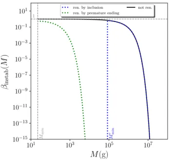
Mmin M 0 min 1 ren. by inclusion ren. by premature endingnot ren.
Figure 4. Mass fraction of PBHs at the end of the instability phase, as a function of the mass at which the black holes form, for ⇢inf = 10 12MPl4 ' 2.43 ⇥ 10
15GeV 4and ⇢ = 10 40M4 Pl'
2.43⇥ 108GeV 4. The black line corresponds to the result obtained before renormalisation and
leads to ⌦PBH(t ) = 8.54 > 1, which is not physical. The blue dotted line is obtained after
renormalisation by inclusion, i.e. when increasing Mmin to Mmin0 such that the integrated mass
fraction ⌦PBH(t ) becomes one. This accounts for the absorption of small-black holes into
larger-mass black holes when the regions that collapse into these large-larger-mass black holes already contain smaller ones. The green dotted line stands for renormalisation by premature ending, i.e. by stopping the instability phase before t , at the time when ⌦PBH reaches one. This accounts for
the fact that if the universe becomes dominated by black holes, the parametric resonance e↵ect stops.
One should note that this inclusion e↵ect might, in practice, prevent ⌦PBHto grow larger than some intermediate value that is smaller than one, but this would have only very little impact on the results derived below as long as that value is of order one (which is expected for the inclusion phenomenon to be significant [45]). Another possibility is that small-black holes are indeed removed from the distribution, but that the decrease in at small M is smoother than a sharp cuto↵ imposed at Mmin0 . In the absence of a clear way to model the formation of PBHs and the inclusion dynamics in the dense regime, it seems difficult to go beyond the sharp cuto↵ procedure, which can however be seen as a limit bounding the range of possible renormalisation procedures (the other bounding procedure being introduced below).
In Fig.4, we have represented the mass fraction at the end of the instability phase for ⇢inf = 10 12MPl4 ' 2.43 ⇥ 10
15GeV 4 and ⇢ = 10 40M4
Pl ' 2.43 ⇥ 10
The black solid line corresponds to what is obtained before renormalisation and leads to ⌦PBH(t ) = 8.54, which is not possible. The blue dotted line represents the result after renormalisation by inclusion (3.12), i.e. by removing the low mass part of the distribution to bring ⌦PBH(t ) back to one.
3.4.2 Renormalisation by premature ending
Another possibility is that, as ⌦PBH increases, PBHs backreact on the dynamics of the universe, which is no longer dominated by the coherent oscillations of the inflaton field, and the instability stops. The precise value of ⌦PBHat which this premature termination occurs is difficult to assess, and for simplicity we will assume it to be one, since our final results mildly depend on it.
In that case, if ⌦PBH(t ) is found to be larger than one, we change the time at which the instability stops,
t ! tinstab, (3.13)
where tinstab is the time at which ⌦PBH reaches one. Therefore, as announced before, there are situations for which tinstab 6= t . The result is displayed in Fig. 4 with the dotted green line. One can check that the large-mass black holes are removed from the mass fraction distribution, since those black holes correspond to scales that enter the instability band towards the end of the instability phase, at which point the instability is now no longer on.
Since, as explained above, the procedure of renormalisation by inclusion removes the small-mass end of the distribution, these two approaches can therefore be viewed as complementaryoverdensity, and by studying the results obtained with both one can assess how much the conclusions depend on the way the mass fraction is renormalised.
The actual renormalisation procedure might lie in between these two schemes: for instance, it could happen that, as ⌦PBH increases, inclusion starts to be important, which slows down the increase of ⌦PBH but does not prevent it from further growing, until the point where premature ending occurs. In such a case, a distribution that is intermediate between the blue and the green curves of Fig. 4 would be obtained. As we will show below, some common conclusions can be drawn with both renormalisation schemes, which motivates the statement that such conclusions are mildly dependent on the renormalisation approach.
3.5 Evolving the mass fraction
After the instability stops, the density of black holes evolves under di↵erent physical e↵ects, such as Hawking evaporation, accretion and merging. In what follows we neglect the two latter and only account for the former. The reason is that accretion and merging are technically difficult to model (see e.g. Refs. [46,47]), and only contribute to enhancing the final value of ⌦PBH. The reason why this is the case for accretion is obvious, and for merging, this is because the Hawking evaporation time (3.6) cubicly depends on the mass. Therefore, when two black holes (say of the same mass) merge, they loose some fraction of their mass through the emission of gravitational waves, but their evaporation time is
100 103 106 109 1/4 tot
(GeV)
10 7 10 6 10 5 10 4 10 3 10 2 10 1 100 PBH BBN = 3 10 32M4 Pl = 10 32M4 Pl = 3 10 33M4 Pl = 10 33M4 Pl = 3 10 34M4 Pl = 10 37M4 PlFigure 5. Integrated mass fraction ⌦PBHas a function of time, here parametrised by the total
energy density ⇢tot, from the end of the instability phase tinstab until BBN, for the same values
of ⇢inf and ⇢ as the ones displayed in Fig.3. For ⇢ = 10 37MPl4 ' (1.4 ⇥ 10
9GeV)4, the mass
fraction needs to be renormalised, which for illustration here is done using the premature-ending procedure.
multiplied by 8, allowing them to live much longer. As a consequence, by only considering Hawking evaporation, we again derive conservative bounds, which underestimate the density of black holes at the epochs where they are observationally constrained.
The mass of a black hole decreases under Hawking evaporation according to [43] M (t, k) = M (tinstab, k) ⇢ 1 t tinstab tevap[M (tinstab, k)] 1/3 , (3.14)
where tevap was given in Eq. (3.6). This expression should be understood as coming with a Heaviside function such that, when t tinstab > tevap, M is set to zero. We do not write it explicitly here for notational convenience. If ¯ denotes the mass fraction in the absence of Hawking evaporation, one then has
⌦PBH(t) = Z Mmax M0 min ¯ (M, t)1 t tinstab tevap(Minstab) 1/3 d ln M , (3.15)
where Minstabis a short-hand notation for M (tinstab, k), and where one should recall that M and k are related through Eq. (3.5). Let us see how ¯ can be calculated (in what follows, quantities with a bar denote their values in the absence of Hawking evaporation).
The energy density of PBHs contained in an infinitesimal range of scales (ln M ) is given by ¯⇢ = ⇢tot¯ (M, t) (ln M). Since PBHs behave as pressureless matter, in the absence of Hawking evaporation one would have ˙¯⇢ + 3H ¯⇢ = 0. Plugging the former expression into the latter, one obtains ( ˙⇢tot+ 3H⇢tot) ¯ (M, t) + ⇢tot˙¯ (M, t) = 0. After the end of the instability phase, we assume that the inflaton instantaneously decays into a radiation fluid, so ¯⇢tot= ¯⇢PBH+ ¯⇢rad. In the absence of Hawking evaporation, one then has ˙¯⇢tot= 3H ¯⇢PBH 4H ¯⇢rad= 3H⌦PBH⇢¯tot 4H(1 ⌦PBH)¯⇢tot= H ¯⇢tot(⌦PBH 4). This gives rise to
˙¯(M, t) + H (⌦PBH 1) ¯(M, t) = 0 . (3.16)
A priori, this equation has to be solved for each mass independently, with the correspond-ing initial condition at tinstab. However, since the equation is linear and does not depend explicitly on the mass, a simpler solution to the problem can be found by introducing the function b that satisfies
˙b + H (⌦PBH 1) b = 0 with b (tinstab) = 1 , (3.17)
and such that
¯ (M, t) = ¯ (M, tinstab) b (t) (3.18)
satisfies Eq. (3.16), with the correct initial condition. The set of equations (3.15), (3.17) and (3.18) then defines a di↵erential system that one can integrate numerically. Finally, let us note that, in practice, we would like to integrate the di↵erential system until a time defined by its energy density rather than its cosmic time (for instance, until BBN defined by ⇢1/4 = ⇢1/4BBN ⇠ 10 MeV). For this reason it is more convenient to use ln ⇢totas the time variable (the log being used for numerical convenience), and Eq. (3.17) becomes
db d ln ⇢tot +
⌦PBH 1
⌦PBH 4b = 0 . (3.19)
The value of cosmic time is still necessary in order to evaluate the Hawking suppression term in Eq. (3.15), which can be tracked solving
d(t tinstab)
d ln ⇢tot =
p 3 MPl
(⌦PBH 4) p⇢tot (3.20)
together with the above system.
In Fig. 5, the solution one obtains for ⌦PBH as a function of time is displayed for the same parameter values as the ones used in Fig. 3. At early time, the e↵ect of Hawking evaporation is negligible, and ⇢PBH/ a 3. If ⌦PBH⌧ 1, ⇢tot' ⇢rad/ a 4and ⌦PBH/ a, otherwise ⇢tot' ⇢PBH/ a 3and ⌦PBHremains equal to one. Let us see when the black holes complete their evaporation. If a PBH forms from a scale that crosses in the instability band at ⇢bc, its mass is given by setting k/kend= (⇢bc/⇢inf)1/6in Eq. (3.5). Inserting the corresponding expression of M into Eq. (3.6), the time tevap tinstab at
which it evaporates can be derived. If ⌦PBH ⌧ 1 until this point, Eq. (3.20) can be integrated and gives ⇢ = ⇢instab[1 + 2
p
⇢instab/3 (t tinstab)/MPl] 2, which means that
the black hole evaporates at the energy density
⇢evap⇠ 1 26244⇠6 ⇣ g 10240 ⌘2 ⇢3 bc M8 Pl . (3.21)
Notice that, in order to obtain this estimate, we have neglected the fact that Hawking evaporation starts before the end of the instability (which was however taken into account for PBHs that entirely evaporate during the instability, see Sec. 3.2). Indeed, given than the collapsing time decays with the initial density contrast, see Eq. (3.1), and since PBHs form in the Gaussian tail of the distribution function where the smaller the density contrast, the more likely it is, most PBHs form close to the end of the instability phase, and for them Hawking evaporation during the instability can be neglected.
If ⌦PBH takes sizeable values before the evaporation of the first black holes, the estimate (3.21) needs only to be corrected by factors of order one (If ⌦PBH = 1, the corrective factor is 8/9). The first black holes to evaporate are the ones with the smallest mass Mmin, i.e. such that ⇢bc = ⇢inf. In Fig. 5, one can check that the evaporation of these PBHs indeed corresponds to the turning point of all curves [for ⇢inf = 10 12MPl4 '
2.43⇥ 1015GeV 4, Eq. (3.21) gives ⇢evap ⇠ 3 ⇥ 10 45MPl4 ' 1.8 ⇥ 10
7GeV 4]. Below this point, Hawking evaporation is efficient and ⌦PBH quickly decreases.
3.6 Reheating through PBH evaporation
The onset of the radiation era, defined as being the time, after the instability phase, after which ⌦PBHremains below 1/2, does not necessarily coincide with tinstab. Indeed, if the universe is dominated by PBHs at the end of the instability, as is the case for
the curve with ⇢ = 10 37M4
Pl ' (1.4 ⇥ 109GeV)4 in Fig. 5, the radiation era only
starts with the evaporation of the first black holes around ⇢⇠ 10 45M4 Pl ' (10
7GeV)4as
explained above. In fact, even if PBHs do not dominate the universe’s content at the end of the instability phase, they may later do so, see the curve with ⇢ = 3⇥ 10 33M4
Pl '
(1.8⇥ 1010GeV)4 in Fig. 5for instance, in which case the onset of the radiation epoch is also delayed.
In such cases, let us point out that the reheating of the universe proceeds from the Hawking evaporation of the PBHs that dominate the energy budget for a transient period after the instability phase.7 If it completes long before BBN, such a mechanism is a priori allowed, and we discuss several of its implications in Sec. 5. It is then inter-esting to extract the energy density at the onset of the radiation period, ⇢rad, from our computational pipeline. Let us notice that ⇢rad is the quantity which is related to what would be defined as the reheating temperature, Treh, through ⇢rad= g⇤⇡2Treh4 /30, where g⇤ is the number of relativistic degrees of freedom.
The quantity ⇢rad is displayed in Fig.6 for ⇢inf = 10 12MPl4 ' (2.43 ⇥ 1015GeV)4
(which is the same value employed in all previous figures, in particular in Fig.5) and as
10 2 101 104 107 1010 1013 1/4
(GeV)
100 103 106 109 1012 1015 1/ 4 ra d(GeV
)
BBN end ren. by inclusion ren. by premature endingFigure 6. Energy density at the onset of the radiation era, ⇢rad, as a function of ⇢ , for
⇢inf= 10 12MPl4 ' 2.43 ⇥ 10
15GeV 4(which is the value used in all previous figures). The blue
curve corresponds to the renormalisation procedure by inclusion, while the green one stands for renormalisation by premature ending. The red circles indicate the location of the discontinuity, i.e. values of ⇢rad comprised between the two circles are never realised, see main text.
a function of ⇢ , which varies between ⇢BBN and ⇢inf. This allows us to identify several relevant regions in parameter space. When ⇢ is large, the instability phase is too short to produce a substantial amount of PBHs and they never dominate the energy content of the universe. This corresponds e.g. to the curve with ⇢ = 3⇥ 10 32MPl4 ' (3.2 ⇥ 10
10GeV)4
in Fig.5. In this case, the radiation era starts when the inflaton decays into radiation, and ⇢rad= ⇢ .
When ⇢ decreases, one first notices in Fig. 6the presence of a discontinuity, that we will explain shortly. In a small range below the discontinuity, ⇢rad is di↵erent from ⇢ , denoting the presence of a phase where PBHs dominate the universe, but does not depend on the renormalisation procedure, revealing that PBHs do not dominate at the end of the instability phase. This corresponds e.g. to the curve with ⇢ = 3⇥10 33MPl4 '
(1.8⇥1010GeV)4in Fig.5. In this case, after the instability phase, there is a first radiation epoch, then PBHs take over and drive a matter epoch, before they evaporate and reheat the universe, which finally enters a second radiation epoch. One then finds ⇢rad< ⇢ .
The discontinuity can be explained as follows: let us consider the case where radi-ation dominates at t , namely ⌦PBH < 1/2 at t . Clearly, in this situation, no renor-malisation is needed since ⌦PBH < 1 at t . Then, as already explained, ⌦PBH grows proportionally to the scale factor until Hawking evaporation becomes efficient and makes
⌦PBH decrease, see Fig. 5. Assume that the maximum value ⌦PBH reaches is slightly smaller than 1/2. In this situation, the start of the radiation epoch is t and ⇢rad= ⇢ since the radiation era is never interrupted. This case corresponds to the upper red dot in Fig.6. Consider now the situation where at the end of the instability, the value of ⌦PBHis infinitesimally larger than in the previous case (and, therefore, still smaller than 1/2 at t ). This means that we now start with a value of ⇢ that is slightly smaller than before (and the instability lasts slightly longer). This gives rise to the same behaviour as described above except that, now, the value at the maximum is slightly larger than before, and above 1/2. This means that the radiation epoch comes to an end and that a matter dominated era starts. Of course, since this is also the time at which Hawk-ing radiation starts to become important, this matter-dominated era lasts a very short amount of time and very soon a new radiation dominated era (the “real” one) starts. The important point, however, is that ⇢radis now very di↵erent from ⇢ and is close to ⇢evap, and this second case corresponds to the lower red dot in Fig.6.
This explains the discontinuity in the curve ⇢rad versus ⇢ . Let us note that an important consequence of this behaviour is the fact that none of the values for ⇢rad comprised between the two red circles can be physically realised. We therefore identify regions in parameter space that are forbidden, not by the observations, but by self-consistency of the scenario itself.
Finally, when ⇢ takes small values, PBHs are very abundantly produced and the mass fraction needs to be renormalised at the end of the instability phase. If renor-malisation is carried out by inclusion, by keeping only the heavy black holes in the distribution, Hawking evaporation proceeds at later times when ⇢ decreases, and the radiation epoch is more and more delayed. There is even a point where the radiation era has not started yet by BBN, which is obviously excluded and which explains why the blue curve is not plotted in Fig.6below that point. If renormalisation is performed by premature ending on the other hand, the result does not depend on ⇢ since ⇢instab becomes independent of that parameter and, from there, the value of ⇢rad is only con-trolled by the evaporation process. In that case, for ⇢1/4 & 286TeV, the onset of the radiation epoch is delayed compared to what it would have been if sourced by inflaton decay. This also implies that the inflaton could decay “inside” the black holes, although due to the no hair theorem, this should not leave any physical imprint. On the other hand, if ⇢1/4 . 286TeV, reheating occurs earlier than it would have with pure inflaton decay.
To conclude this section, let us stress again that, for ⇢ . 1010GeV and ⇢inf = 10 12M4
Pl ' 2.43 ⇥ 1015GeV 4
(a full scan of the parameter space is presented in the following), namely below the lower red point in Fig. 6, the radiation in our universe no longer comes from inflaton decay but from the evaporation of PBHs formed during preheating. Given the generic character of the situation considered here (single-field inflation with quadratic minimum), this is clearly one of the main conclusions of the present paper.
3.7 Planckian relics
The previous considerations show that the universe may have gone through a phase where PBHs are numerous, and can even dominate the energy budget of the universe, but that these black holes can also well have all disappeared before BBN, through Hawking evaporation. In such a case, there is no direct way to constrain them, unless they do not fully evaporate and leave some relics behind.
This possibility has been discussed [52, 53] in the context of quantum-gravity in-spired scenarios, where it has been suggested that black hole evaporation might stop when the mass of the black hole reaches the Planck mass. In this case, the number density of black hole can be computed at the end of the instability phase according to
nPBH(tinstab) = ⇢tot
Z Mmax
Mmin
˜ (M, tinstab)
M d ln M . (3.22)
In this expression, ˜ (M, tinstab) corresponds to Eq. (3.8) (with t replaced with tinstab) where, instead of taking max as being the minimum value between one and the right-hand side of Eq. (3.7), one simply takes max= 1. This ensures that the black holes that evaporate before the end of the instability phase are also accounted for in the calculation of relics.
Since this number density is not a↵ected by Hawking evaporation, it then evolves according to the function b(t) introduced in Sec.3.5, i.e. solely under the e↵ect of cosmic expansion. The fractional energy density of relics at subsequent times is thus given by
⌦relics(t) = b(t)
Z Mmax
Mmin
˜ (M, tinstab)MPl
M d ln M . (3.23)
Let us note that this expression assigns one Planckian relic to each black hole, whether it has already evaporated or not. It therefore gives the density of “naked” relics only in the late-time limit, when all black holes have evaporated. It however always provides a lower bound on the contribution to dark matter (DM) originating from black holes and their relics, and as such, should be checked to be smaller than ⌦DM, which will be done in Sec.4.3.
4
Observational consequences
Having described the physical setup and the methods employed to model it, let us now turn to the results and discuss their physical implications.
4.1 The onset of the radiation era
In Sec.3.6, it was found that in some cases, the production of PBHs is so efficient that they may come to dominate the energy budget of the universe, either before the end of the instability phase or afterwards. In that case, the onset of the radiation era does not correspond to the time when the inflaton decays, i.e. when ⇢ = ⇢ , but rather occurs
101 102 105 108 1011 1014 1/4 inf(GeV) 101 102 105 108 1011 1014 1/ 4 (GeV ) Renormalisation by inclusion < ⇢1/4 BBN 100 103 106 109 1012 1015 1/ 4 ra d(GeV ) 101 102 105 108 1011 1014 1/4 inf(GeV) 101 102 105 108 1011 1014 1/ 4 (GeV )
Renormalisation by premature ending
< ⇢1/4 BBN 100 103 106 109 1012 1015 1/ 4 ra d(GeV )
Figure 7. The energy density at the onset of the radiation era as a function of ⇢inf and ⇢ .
The grey region is excluded since it corresponds to ⇢inf < ⇢ . Left panel: renormalisation by
inclusion. Right panel: renormalisation by premature ending.
when the PBHs evaporate. The corresponding energy density, ⇢rad, has been displayed as a function of ⇢ and for a fixed value of ⇢inf in Fig.6.
In Fig. 7, the same quantity is shown, but as a function of both ⇢inf and ⇢ . Thus Fig. 6 is a vertical slice of Fig. 7. The left panel corresponds to renormalisation by inclusion, see Sec.3.4.1, while the right panel stands for renormalisation by premature ending, see Sec.3.4.2. The grey region is excluded since it corresponds to ⇢ > ⇢inf. In the region where ⇢rad= ⇢ , PBHs never dominate and reheating occurs at the end of the instability phase, through decay and thermalisation of the inflaton. In both figures, the lower right triangular regions, in which ⇢rad6= ⇢ , are such that reheating proceeds by PBH evaporation. Notice that, there, the darkest blue region corresponds to parameter values for which the universe is still not dominated by radiation at BBN, which is
excluded. This allows us to generalise the remarks made around Fig. 6: when ⇢ is
large, the instability phase is short, PBHs never dominate the universe, so ⇢rad= ⇢ and reheating proceeds in the standard way; when ⇢ is sufficiently small, PBHs can dominate the universe, which results into either delaying or anticipating the universe reheating. For ⇢1/4inf ' 1015GeV, which corresponds to a tensor-to-scalar ratio of r' 10 3, reheating occurs from PBHs evaporation when ⇢1/4. 2 ⇥ 109GeV.
More generally, the boundary of the lower-right triangles, i.e. the condition for reheating the universe via PBH evaporation, can be worked out as follows. Clearly, reheating proceeds through PBHs evaporation if the PBHs are formed in a substan-tial way. This is the case if the critical density contrast given in Eq. (3.4), c ⇠ (3⇡/2)2/3(k/kend) 2(⇢inf/⇢instab) 1/3 = (3⇡/2)2/3(⇢instab/⇢bc)1/3 [where we have used k/kend = (⇢bc/⇢inf)1/6] is much smaller than p2P . Moreover, the modes that get the more amplified are the ones that enter the instability band the earlier, and thus exit the Hubble radius not long before the end of inflation. For them, one can take
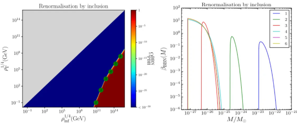
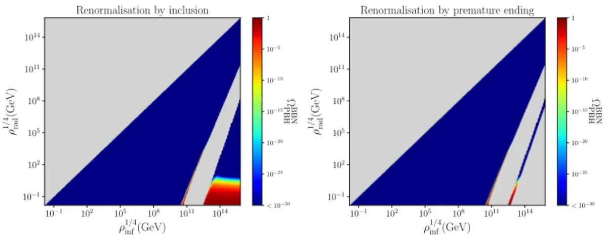
101 102 105 108 1011 1014 1/4 inf(GeV) 101 102 105 108 1011 1014 1/ 4 (GeV ) Renormalisation by inclusion 1 2 3 4 5 6 < 1030 1025 1020 1015 1010 105 1 BBN PBH 1027 1026 1025 1024 10 23 10 22 10 21 M/M 10 6 10 5 10 4 10 3 10 2 10 1 100 101 102 BBN (M ) Renormalisation by inclusion 1 2 3 4 5 6
Figure 8. In the left panel, the fraction of the universe made of PBHs at BBN is displayed as a function of ⇢inf and ⇢ , when the mass fraction is renormalised by inclusion. The grey region
corresponds to ⇢ > ⇢inf and is therefore forbidden. In the blue region, ⌦BBNPBH < 10 30, which
leaves the parameters unconstrained. In the dark red region, ⌦BBN
PBH ' 1, which is excluded. In
between, there is a fine-tuned region where ⌦BBN
PBH takes fractional values, and where the details
of the mass fraction matter. For that reason, 6 points are labeled across that region, for which ⌦BBN
PBH= 10 2, and their mass fraction is shown in the right panel.
P⇣,end ⇠ Hend2 /(8⇡2MPl2), see Eq. (2.8), hence P,bc ⇠ 3⇢inf/(50⇡
2M4
Pl), see Eq. (3.10).
As a consequence, the condition c/p2P ⌧ 1 leads an upper bound on ⇢instab, namely
⇢instab < 4(125
p
3 ⇡5) 1(⇢inf/MPl4)
3/2⇢
bc. This makes sense since, in order to have size-able PBHs production, the instability must last long enough and, therefore, ⇢instabmust be small enough. Since ⇢bc< ⇢inf and ⇢ < ⇢instab by construction, this gives rise to
⇢ M4 Pl < 4 125p3 ⇡5 ✓ ⇢inf M4 Pl ◆5/2 . (4.1)
One can check that this expression provides a good fit to the boundary of the lower right triangular regions in Fig. 7, hence it gives a simple criterion to check whether or not reheating proceeds via PBH evaporation.
4.2 Constraints from the abundance of PBHs
Let us now discuss observational constraints from the predicted abundance of PBHs. The amount of DM made of PBHs is constrained by various astrophysical and cosmo-logical probes, through their evaporation or gravitational e↵ects (for a recent review, see e.g. Ref. [29, 30]). The earliest constraint, i.e. the one limiting black holes with the smallest mass, is BBN. This is why in the left panels of Figs.8and9, the fraction of the universe made of PBHs at BBN is displayed, as a function of ⇢inf and ⇢ .
As before, the model is defined only when ⇢ < ⇢inf, i.e. outside the grey region. The parameter space is otherwise essentially divided into two main regions: in the dark
101 102 105 108 1011 1014 1/4 inf(GeV) 101 102 105 108 1011 1014 1/ 4 (GeV )
Renormalisation by premature ending
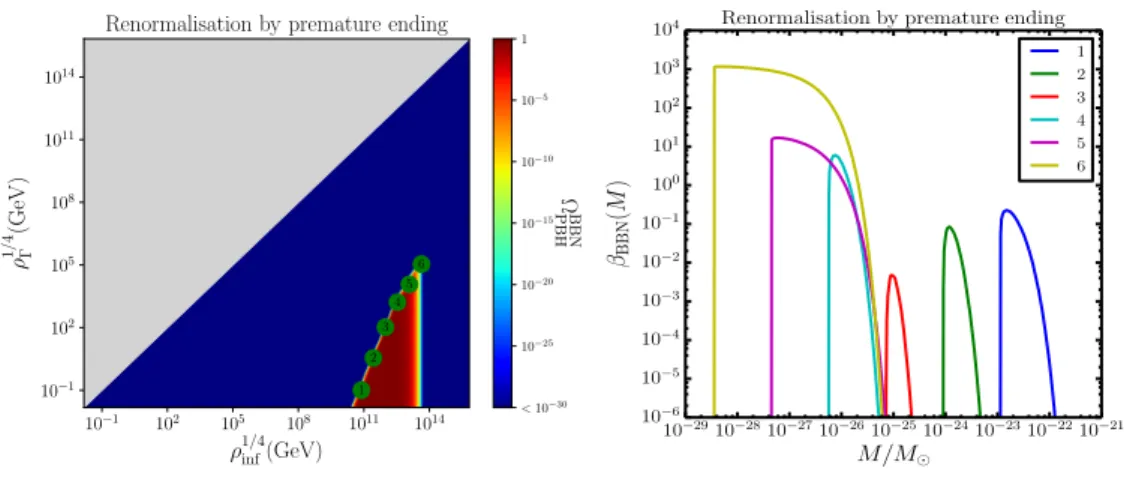
1 2 3 4 5 6 < 1030 1025 1020 1015 1010 105 1 BBN PBH 10 2910 2810 2710 2610 2510 2410 2310 2210 21 M/M 10 6 10 5 10 4 10 3 10 2 10 1 100 101 102 103 104 BBN (M )
Renormalisation by premature ending
1 2 3 4 5 6
Figure 9. Same as in Fig.8, when the mass fraction is renormalised by premature ending.
blue region, i.e. for large values of ⇢ , ⌦BBNPBH . 10 30, and all observational constraints are easily passed. This corresponds to situations where PBHs are either not substantially produced, or evaporate before BBN. In the dark red region, i.e. for smaller values of ⇢ , ⌦BBNPBH' 1 and the universe is not radiation dominated at the time of BBN, which is not allowed at more than the few percents level [54]. A substantial fraction of the reheating parameter space can therefore be excluded from the considerations presented in this work, which is our second main result. For instance, for the typical value ⇢1/4inf ' 1015GeV, ⌦BBN
PBH& 0.1 if ⇢ 1/4
. 1.6 ⇥ 107GeV when renormalisation is performed by inclusion. The location of the boundary between the excluded and the allowed regions can be worked out as follows. Requiring that the evaporation time, estimated in Eq. (3.21), is later than BBN leads to ⇢bc/MPl4 < (9⇥ 6
2/3)⇠2(10240/g)2/3(⇢
BBN/MPl4)
1/3. In ad-dition, we must also make sure that the corresponding PBHs have been produced in a non-negligible quantity which leads to the upper bound on ⇢instab derived in the text above Eq. (4.1). Combining these two expressions, one obtains ⇢instab/MPl4 < (36⇥
62/3⇠2)/(125p3 ⇡5)(10240/g)2/3(⇢
BBN/MPl4)1/3(⇢inf/MPl4)3/2 ⇠ 2.5 ⇥ 10 29(⇢inf/MPl4)3/2.
Combined with Eq. (4.1), this gives rise to ⇢instab MPl4 < min " 6.0⇥ 10 5 ✓ ⇢inf MPl4 ◆5/2 , 2.5⇥ 10 29 ✓ ⇢inf MPl4 ◆3/2# . (4.2)
One can check that this rough estimate indeed provides a good enough description of
the boundary between the blue and the red regions in Fig. 8 where one simply has
⇢instab = ⇢ (the situation in Fig. 9 is more complicated since those are two di↵erent
quantities).
In between the excluded and the allowed regions, there is a fine-tuned, thin line along which ⌦BBNPBH can take fractional values. There, the details of the mass fraction, i.e. the value of and the range of masses it covers, matter. For this reason, both in
101 102 105 108 1011 1014 1/4 inf(GeV) 101 102 105 108 1011 1014 1 /4 (GeVrad ) Renormalisation by inclusion < 1030 1025 1020 1015 1010 105 1 BBN PBH 101 102 105 108 1011 1014 1/4 inf(GeV) 101 102 105 108 1011 1014 1 /4 (GeVrad )
Renormalisation by premature ending
< 1030 1025 1020 1015 1010 105 1 BBN PBH
Figure 10. Fraction of the universe made of PBHs at BBN, as a function of ⇢inf and ⇢rad, when
the mass fraction is renormalised by inclusion (left panel) and premature ending (right panel). The grey region is not realised either because ⇢rad> ⇢inf, or because the corresponding value of
⇢rad is never realised, see the discussion around Fig.6.
Figs.8and9, we have sampled 6 points along this thin line, for which ⌦BBNPBH = 10 2, and we show the corresponding mass fraction in the right panels, as a function of M/M . We have checked that fixing ⌦BBNPBH to values di↵erent than 10 2 does not qualitatively change the following remarks.
First, one may be surprised that some values of are larger than one. This is
because, although at the end of the instability is smaller than one by definition, see Eq. (3.8), it is then redshifted by b, see Eq. (3.18), which can be much larger than one. The integrated mass fraction, ⌦PBH, does always remain smaller than one.
Second, the observational constraints on the value of depend on whether the
mass distribution is monochromatic (i.e. all black holes have the same mass) or ex-tended. In our case, it is clearly extended, and the constraints then depend on its precise profile. Let us however note [29] that the smallest mass being constrained is of the order 10 24M . Only the points labeled 1 and 2 in Figs. 8 and 9, i.e. the ones with ⇢inf ⇠ 10 30MPl4 ' (7.7 ⇥ 10
10GeV)4 and very small values of ⇢ , can there-fore be constrained. More precisely, for monochromatic mass distributions, one has8 BBN(10 24M < M < 10 23M ) < 10 7 and BBN(10 23M < M < 10 19M ) <
8Observational constraints are usually quoted at the time of formation, assuming that PBHs form in
the radiation era. In the present setup, PBHs form in a matter-dominated phase, so it is more convenient
to express BBN constraints at the time of BBN itself. In terms of the mass fraction ˜format the time
of formation in the case where the universe is radiation dominated between PBH formation and BBN (i.e. the quantity quoted in most reports on observational constraints), it is given by
BBN= 31/4 p 4⇡⇠ ✓ M6 Pl M2⇢BBN ◆1/4 ˜form. (4.3)
101 102 105 108 1011 1014 1/4 inf(GeV) 101 102 105 108 1011 1014 1/ 4 (GeV ) Renormalisation by inclusion < 103 102 101 > 1 re lic/ DM 101 102 105 108 1011 1014 1/4 inf(GeV) 101 102 105 108 1011 1014 1/ 4 (GeV )
Renormalisation by premature ending
< 103 102 101 > 1 re lic/ DM
Figure 11. Abundance of Planckian relics normalised to the one of dark matter, as a function of ⇢inf and ⇢ , when the mass fraction is renormalised by inclusion (left panel) and premature
ending (right panel).
10 12. Although this would have to be adapted to the extended mass distributions we are dealing with, this confirms that the points labeled 1 and 2 are probably excluded. This however does not change the main shape of the excluded region.
Third, no black hole with masses larger than 10 20M are produced unless they
are too abundantly produced. This implies that the present scenario cannot
ac-count for merger progenitors as currently seen in gravitational-wave detectors such as LIGO/VIRGO, nor can it explain dark matter since such black holes have all evaporated by now.
In Fig. 10, we finally display ⌦PBH at BBN as a function of ⇢inf and ⇢rad, in order to derive constraints in that parameter space too. As above, the upper-left grey triangle corresponds to ⇢rad> ⇢infand is therefore to be discarded. There are however additional grey regions corresponding to values of ⇢rad that are not realised: an intermediate grey band that stands for the discontinuity gap commented on around Fig.6, and in the case of renormalisation by premature ending, a lower right grey triangle that arises from the saturation e↵ect discussed around Fig.6as well.
4.3 Constraints from the abundance of Planckian relics
In Sec. 3.7, we discussed the possibility that evaporated PBHs leave Planckian relics behind, i.e. objects of mass ⇠ MPl that do not further evaporate. If they exist, their
density is expressed in Eq. (3.23), and it should be smaller than the one of dark matter. This is why in Fig. 11, the ratio ⌦relic/⌦DM is displayed, as a function of ⇢inf and ⇢ , and in Fig.12, as a function ⇢inf and ⇢rad. Similarly to Fig. 10, one can see that parameter space is essentially divided into two regions: one (dark blue) where the amount of Planckian relics left over from PBHs is negligible, and one (dark red) that is excluded since Planckian relics overtake the dark matter abundance. From Fig.11, we see that,
101 102 105 108 1011 1014 1/4 inf(GeV) 10 1 102 105 108 1011 1014 1 /4 (GeVrad ) Renormalisation by inclusion < 103 102 101 > 1 relic / DM 101 102 105 108 1011 1014 1/4 inf(GeV) 101 102 105 108 1011 1014 1 /4 rad (GeV )
Renormalisation by premature ending
< 103 102 101 > 1 relic / DM
Figure 12. Abundance of Planckian relics normalised to the one of dark matter, as a function of ⇢inf and ⇢rad, when the mass fraction is renormalised by inclusion (left panel) and premature
ending (right panel).
if ⇢1/4inf ' 1015GeV, then ⌦
relics > ⌦DM if 1.4⇥ 108GeV . ⇢1/4 . 3.7 ⇥ 109GeV and
renormalisation is performed by inclusion. If it is performed by premature ending, then ⌦relics > ⌦DM if ⇢1/4 . 3.7 ⇥ 109GeV. Further regions of parameter space can thus be excluded from the predicted abundance of relics, if they exist. In between the excluded and allowed regions, there is a fine-tuned boundary where Planckian relics could constitute a substantial fraction of the dark matter.
5
Discussion and conclusions
In this work, we have shown how the coherent oscillations of the inflaton field around a local minimum of its potential at the end of inflation can lead to the resonant amplifica-tion of its fluctuaamplifica-tions at small scales, that can then collapse and form PBHs. We have shown how the abundance and mass distribution of these PBHs can be calculated from the spectrum of fluctuations as predicted by inflation. In some cases, it was found that the production mechanism is so efficient that one needs to account for possible inclusion e↵ects, and/or for the possibility that PBHs backreact and prematurely terminate the preheating instability. In such cases, the universe undergoes a phase where it is domi-nated by a gas of PBHs, that later reheats the universe by Hawking evaporation. This happens when Eq. (4.1) is satisfied.
A first result obtained in the present paper is therefore that, in the most simple models of inflation, reheating does not necessarily occur via inflaton decay, but for a large fraction of parameter space, it rather proceeds from the evaporation of PBHs produced during preheating. For the iconic value ⇢1/4inf ' 1015GeV (corresponding to a tensor-to-scalar ratio r⇠ 10 3), this is the case provided ⇢1/4
. 2⇥109GeV. This deeply modifies our view of how the universe is reheated in the context of the inflationary theory: the
10 1 102 105 108 1011 1014 1/4 inf(GeV) 10 1 102 105 108 1011 1014 1/ 4 (GeV ) Renormalisation by inclusion not realised ⌦relic> ⌦DM ⌦BBN PBH> 0.1 10 1 102 105 108 1011 1014 1/4 inf(GeV) 10 1 102 105 108 1011 1014 1/ 4 (GeV )
Renormalisation by premature ending
not realised
⌦relic> ⌦DM
⌦BBN PBH> 0.1
Figure 13. Combined constraints in the the space (⇢inf, ⇢ ), when the mass fraction is
renor-malised by inclusion (left panel) and premature ending (right panel). Red regions are excluded since they yield a too large abundance of primordial black holes. If black holes leave Planckian relics behind after evaporation, the blue regions are also excluded since they lead to too many of them. The remaining region, displayed in white, is the allowed one.
radiation in our universe could well originate from Hawking radiation rather than from inflaton decay as usually thought.
A second result concerns the constraints on the energy scale of inflation and the en-ergy at the onset of the radiation-dominated epoch that follow from the above-described mechanism. These combined constraints on the two parameters describing our setup, either ⇢inf and ⇢ or ⇢inf and ⇢rad, are given in Fig. 13 and Fig. 14 respectively. All coloured regions are excluded: the grey one since it corresponds to values of ⇢ and/or ⇢rad that cannot be realised; the red one since it leads to an overproduction of PBHs that is excluded by observations; and, if evaporated black holes leave Planckian relics behind, the blue one since it yields more relics than the measured abundance of dark matter. Only the white region remains, which strongly constrains the energy scale of inflation and reheating. For ⇢1/4inf ' 1015GeV, if renormalisation is performed by inclu-sion, values such that ⇢1/4. 2 ⇥ 109GeV and 1.4⇥ 108GeV. ⇢1/4. 3.7 ⇥ 109GeV are excluded. If renormalisation is performed by premature ending, then values such that ⇢1/4 . 3.7 ⇥ 109GeV are excluded. The constraints on ⇢
rad are also relevant since, as already mentioned, they correspond to constraints on the reheating temperature. For ⇢1/4inf ' 1015GeV, if renormalisation is performed by inclusion, we find that only values such that 102MeV. ⇢1/4
rad . 3 ⇥ 102GeV and ⇢ 1/4
rad & 4 ⇥ 109GeV are allowed. If renor-malisation is performed by premature ending, then only ⇢1/4rad& 4 ⇥ 109GeV is possible.