HAL Id: hal-00295464
https://hal.archives-ouvertes.fr/hal-00295464
Submitted on 8 Jul 2004
HAL is a multi-disciplinary open access
archive for the deposit and dissemination of
sci-entific research documents, whether they are
pub-lished or not. The documents may come from
teaching and research institutions in France or
abroad, or from public or private research centers.
L’archive ouverte pluridisciplinaire HAL, est
destinée au dépôt et à la diffusion de documents
scientifiques de niveau recherche, publiés ou non,
émanant des établissements d’enseignement et de
recherche français ou étrangers, des laboratoires
publics ou privés.
R. Lemoine
To cite this version:
R. Lemoine. Secondary maxima in ozone profiles. Atmospheric Chemistry and Physics, European
Geosciences Union, 2004, 4 (4), pp.1085-1096. �hal-00295464�
SRef-ID: 1680-7324/acp/2004-4-1085
Chemistry
and Physics
Secondary maxima in ozone profiles
R. LemoineRoyal Meteorological Institute of Belgium, 3, Avenue Circulaire, 1180 Brussels, Belgium Received: 9 January 2004 – Published in Atmos. Chem. Phys. Discuss.: 23 March 2004 Revised: 28 June 2004 – Accepted: 30 June 2004 – Published: 8 July 2004
Abstract. Ozone profiles from balloon soundings as well as
SAGE II ozone profiles were used to detect anomalous large ozone concentrations of ozone in the lower stratosphere. These secondary ozone maxima are found to be the result of differential advection of ozone-poor and ozone-rich air asso-ciated with Rossby wave breaking events. The frequency and intensity of secondary ozone maxima and their geographical distribution is presented. The occurrence and amplitude of ozone secondary maxima is connected to ozone variability and trend at Uccle and account for a large part of the total ozone and lower stratospheric ozone variability.
1 Introduction
Laminated ozone structures in the lower stratosphere have long been observed in ozone vertical profiles. Laminae ob-served in ozone vertical profiles from ozonesondes, are local extrema of the ozone concentration, situated in the lowermost part of the stratosphere. A lamina can be a local maximum or minimum of the concentration with a limited vertical ex-tent of typically a few hundreds of meters. In some circum-stances several laminae can be observed in one profile. In this case, layers of ozone-poor and ozone-rich air alternate. A secondary ozone maximum is the extreme case of a lam-ina where the maximum in the lower stratosphere is the same order of magnitude as the mid-stratospheric ozone concentra-tion maximum. The associated minimum is well pronounced with concentrations well below the average.
Laminae in ozone profiles are very common at mid lat-itudes (Appenzeller and Holton, 1997) and have been the subject of many studies (Mlch and Lavstovivcka (1996) and references therein). Some studies consider laminae and sec-ondary maxima in ozone vertical profiles separately while
Correspondence to: R. Lemoine
others do not. The border line between laminae and sec-ondary maxima can only be chosen arbitrarily, as all ampli-tudes and depths of ozone rich and poor layers exist between the finest lamina to the large secondary maximum.
Different approaches seem to coexist in the literature. The first, introduced by Dobson (1973) and supported by Varot-sos et al. (1994) suggests that laminae are created through stratosphere-troposphere exchange near the subtropical jet stream.
The second view (Reid and Vaughan, 1991) presents dif-ferential advection of air from different locations as the likely origin for laminae. As this process is most active at high lati-tudes in winter and spring, Reid and Vaughan (1991) rule out the suggestion made by Dobson (1973) that laminae orig-inate near the subtropical jet stream. Instead, the authors suggested that folds beneath the polar night jet might form laminae near the edge of the polar vortex. Although the possibility remains that a small number of laminae may be generated by stratosphere-troposphere exchange, Reid and Vaughan (1991) suggested that laminae may represent evi-dence of a process that can cause exchange of air in and out of the polar vortex.
Reid and Vaughan (1991) and Reid and Vaughan (1993) define ozone laminae as features between 200 m and 2.5 km in vertical extent which form a distinct layer of magnitude greater than 20m Pa. They found that laminae are most com-monly found between 12 and 18 km at high latitudes in wter and spring. The abundance and amplitude of laminae in-crease with increasing latitude and the thickness dein-creases with increasing latitude. For the origin of laminae, they sug-gested that a mechanism operates at the lower edge of the polar vortex (where ozone mixing ratio increases sharply on isentropic surfaces) which transports ozone to middle latitude in the form of laminae, particularly during spring when the polar vortex dissipates. Possible candidates for this mechanism are inertia-gravity waves associated with the sub-tropical jet stream as proposed by Danielsen et al. (1991) or
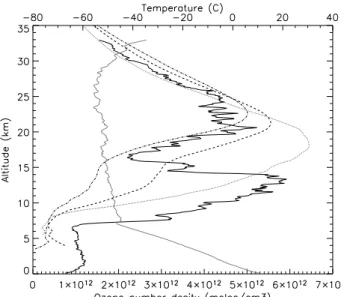
Fig. 1. Example of ozone secondary maxima observed in an ozone sounding on April 19, 2002 at Uccle. For comparison, SAGE II mean ozone profiles are shown for 30-40◦N (dot-dashed curve), 40-50◦N (dashed curve) and 60-70◦N (dotted curve). The grey curve is the air temperature.
distortions of the polar vortex boundary by synoptic scale motions as proposed by Tuck et al. (1992).
Reid et al. (1994), using the EASOE ozonesonde archive, analyzed the occurrence of laminae in the course of the 1992 winter confirming the findings of Reid and Vaughan (1991) and Reid and Vaughan (1993). Laminae are most abundant near the edge of the polar vortex and are generally absent above 430 K inside the vortex. Observation of inertia-gravity waves in the lower stratosphere appears to suggest that such waves are not of sufficiently large amplitude to cause the kind of laminae that are observed.
Yet another approach to this phenomena is to use La-grangian techniques to study laminated features in the ozone field. Plumb et al. (1994) and Waugh et al. (1994) used Lagrangian techniques to study the behavior of trace con-stituents in the boundary of the lower stratospheric vortex. Plumb et al. (1994) showed that vortex intrusions also occur during strong ridging events, during which the vortex is dis-rupted by one or several large-scale ridges. Such intrusions can lead to the formation of elongated thin filaments of mid-latitude air inside the vortex.
Appenzeller and Holton (1997) determined regions in the middle atmosphere where the abundance of ozone laminae or laminae in a tracer distributed as potential vorticity (PV) is expected to be high. They estimated that laminae generation is expected to be most efficient where vertical wind shears coexist with tracer horizontal gradients.
In contrast with most of the above mentioned articles, this paper concentrates on laminae of larger vertical extent, of-ten referred to as secondary ozone maxima. This paper is
organised as follows. Sect. 2 presents the data used in this study. Sect. 3 gives the definition of a secondary ozone max-imum and two examples are given in Sect. 4. The relation between the occurrence of ozone secondary maxima and the atmospheric circulation is developed in Sect. 5. Sections 6 and 7 present an in-depth analysis of ozone secondary max-ima observed in ozone soundings at Uccle (Belgium) and in SAGE II ozone profiles. Sect. 8 describes the possible link between ozone trends and the occurrence of ozone secondary maxima.
2 Dataset description
Ozone soundings have been performed at Uccle, Belgium, since 1969 three times a week with two main interruptions in 1985 and 1986. Brewer-Mast ozone sensors were used from the beginning until March 1997 when it was decided to use model Z ECC ozone sensors. The vertical resolution of an ozone sounding is better than a few 100 meters. Given the high vertical resolution, ozonesondes are the most suitable instrument to study laminated structures in the lower strato-sphere. A complete comparison between Uccle ozone pro-files and SAGE II ozone propro-files was performed by Lemoine and De Backer (2001).
The Stratospheric Aerosol and Gas Experiment II (SAGE II) is a seven-channel sun spectrophotometer launched in October 1984 aboard the NOAA ERBS satellite. SAGE uses the solar occultation technique that measures the attenuation of the solar radiation by the Earth’s atmosphere at the limb due to scattering and absorption by different at-mospheric species, primarily at 600 nm (Mc Cormick, 1987). During each spacecraft sunrise and sunset SAGE II provides water vapour, ozone, nitrogen dioxide and aerosol extinction profiles. The resolution of the instrument is not homoge-neous, with a horizontal extent of the measurement of 200 km along the line of sight and 2.5 km in the perpendicular direc-tion. The vertical resolution is set to 0.5 km in data version 6.0 and profiles extend from the tropopause up to 60 km alti-tude.
We used geopotential height, potential vorticity maps and wind fields to analyse the synoptic weather situation for a number of case studies. These data were provided by the European Center for Medium-range Weather Forecast.
3 Definition of an ozone secondary maximum
In this study, we only consider ozone secondary maxima. We define an ozone secondary maximum as a layer of ozone-rich air where the ozone partial pressure is at least 75% of the ozone pertial pressure at the main maximum and that is separated from the main maximum by a layer of ozone-poor air where the ozone partial pressure is at most 75% that of the secondary maximum. There are no upper or lower lim-its on the thickness of the ozone-poor and ozone-rich layers.
(a) (b)
(c) (d)
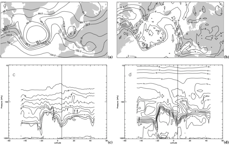
Fig. 2. Synoptic situation on 20020419 extracted from ECMWF analysis. (a) 250 hPa geopotential height (105m2/s2) and (b) 330 K potential vorticity (PVU). The location of Uccle is marked with an x. Cross-sections between −45 and +45◦longitude at 50◦N. (c) potential vorticity (PVU) and (d) ozone partial pressure (mPa). The vertical line in the bottom figures correspond to the Uccle longitude.
In order to be used in this survey, the ozone sounding must have reached the 20 hPa level to ensure that the main ozone maximum was measured. The same criteria are applied to SAGE II profiles to detect secondary maxima. The lower ver-tical resolution of the SAGE profiles should have little or no influence on the detection of secondary maxima: given the usually observed thickness of the ozone-rich and ozone-poor layers (see Sect. 4), secondary ozone maxima are resolved by SAGE.
4 Example
On April 19, 2002 a particularly remarkable secondary ozone maximum was observed in an ozone sounding at Uccle. The geopotential height and PV charts (Fig. 2a and b) show a ridge associated with low-PV air on the Eastern Atlantic and a trough region associated with high-PV air above Western Europe. This trough is limited to the very lower stratosphere and is not visible in geopotential height and PV maps above 100 hPa.
Longitude-height cross sections of the PV and ozone fields at 50◦N shown in Fig. 2c and d are extremely similar to
Fig. 10 in O’Connor et al. (1999). The intrusion between 20◦W and 0◦W is clearly visible in both the PV and ozone fields and extends up to 350 K. On the other and, the sec-ondary ozone maximum above Uccle (5◦E) is well resolved
in the ozone field as ozone-rich air underneath ozone poor air but it is not present in the PV field.
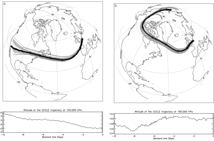
Ten days isentropic backward trajectories were computed with the FLEXTRA model and ECMWF wind fields analy-ses. Clusters of trajectories were used to check the reliability of the result. Isentropic trajectory clusters ending at 200 hPa and 90 hPa above Uccle on 19 April 2002 are presented in Fig. 3a and b. Trajectories ending at 200 hPa correspond to the secondary ozone maximum and trajectories ending at 90 hPa correspond to the associated ozone minimum.
The trajectories ending at 90hPa have their origin near (30◦N, 110◦W) around 70 hPa, in the lower stratosphere. The ozone partial pressure measured by the ozonesonde agrees with ozone values from the ECMWF assimilated ozone data. Higher up in the stratosphere, additional tra-jectory calculations (not shown) showed that the atmosphere up to 50 hPa is made of air that was advected from close to 30◦N.
Fig. 3. 10 days isentropic back trajectory clusters and altitude of the trajectory ending above Uccle. Clusters are made of 25 trajectories with end points on a 2 by 2 degree grid centered on Uccle and spaced by 0.5 degree. (a) trajectories ending at 100hPa on 20020419 12:00 UT. (b) trajectories ending at 160hPa on 20020419 12:00 UT. The pressure levels correspond to the pressure at which the secondary ozone maximum and minimum were observed in the sounding.
The trajectories corresponding to the secondary maximum have their origin north of the arctic circle and well inside the polar vortex, according to PV maps. The ozone rich air mass above Uccle on 19 April 2002 is thus associated with a low geopotential trough and a equatorward intrusion of high ozone concentration and high PV air from the base of the polar vortex. The ozone-poor air at 100 hPa is associated with low latitude stratospheric air that extends up to at least 30 hPa. The presence of the poleward and equatorward in-trusion create an strong disruption of the base of polar vortex edge which is turned in a North-South direction. The pertur-bation is not present at higher altitudes where the wave has not (yet) propagated. The vertical wind shear induced is well captured in Fig. 3 where the 200 hPa trajectory turns at a right angle one day before passing over Uccle while the 100 hPa trajectory does not. It is important to note that the wind shear is not obvious in the sounding data in this case. More gener-ally, there is no systematic association of secondary maxima with an important wind shear in ozone soundings. The rea-son is that secondary ozone maxima are most pronounced downstream of the frontal region where the wind shear is no more present.
5 Secondary ozone maxima and Rossby wave breaking
In the northern hemisphere, planetary-scale Rossby waves constitute a primary source of dynamical variability. Given the long chemical lifetime of ozone in the lower stratosphere, reversible transport associated with Rossby waves accounts for the largest part of ozone variability in winter and spring. In addition to reversible transport, irreversible transport oc-curs during Rossby wave breaking events. Such events are associated with troposphere-stratosphere exchange and tropopause folds. Wave breaking events can be classified as either “equatorward” or “poleward”. On potential vorticity maps, equatorward breaking events, tongues of high poten-tial vorticity (PV) air extend equatorward and in poleward events, tongues of low PV air extend poleward.
Peters and Waugh (1996) studied a number of Rossy-wave-breaking events which resulted in the poleward ad-vection of upper tropospheric air from the subtropics dur-ing winter. They identified two types of poleward breakdur-ing: type 1 (P1) in which the intruded tropospheric air tilts up-stream, thins and is advected cyclonically and type 2 (P2) in which the air tilts downstream, broadens and wraps up
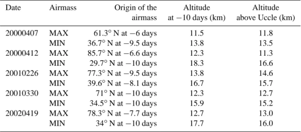
Table 1. Altitudes and latitudes of the back trajectories calculated for the ozone-rich (MAX) and ozone-poor (MIN) air-masses observed with a secondary ozone maximum. All trajectories end above Uccle (50.8◦N, 4.35◦E.)
Date Airmass Origin of the Altitude Altitude airmass at −10 days (km) above Uccle (km) 20000407 MAX 61.3◦N at −6 days 11.5 11.8 MIN 36.7◦N at −9.5 days 13.8 13.5 20000412 MAX 85.7◦N at −6.6 days 12.3 11.3 MIN 29.7◦N at −10 days 18.3 16.6 20010226 MAX 77.3◦N at −9.5 days 13.8 14.6 MIN 39.6◦N at −8.1 days 16.7 15.7 20010330 MAX 71◦N at −10 days 12.3 12.7 MIN 34.5◦N at −10 days 15.9 15.2 20020419 MAX 78.3◦N at −7.7 days 12.7 13.0 MIN 34◦N at −10 days 17.7 16.0
anticyclonically. P1 breakings are expected on the cyclonic side of jets and P2 on the anticyclonic side. The authors ob-served that Rossby waves propagate along the jet and break in the region of weak zonal winds. They also noted that the wave breaking events occurred in two preferred locations that are consistent with the preferred regions of blocking: At-lantic Ocean/Europe and Pacific Ocean/North America.
P2-type wave-breaking events can lead to the advection of air from close to the subtropical jet stream into the mid-latitude lower stratosphere. This mechanism can lead to the formation of ozone secondary maxima, as was shown by O’Connor et al. (1999). In the two case-studies presented in that paper, breaking events led to irreversible transport of air from the subtropics to the mid-latitudes, up to 365 K po-tential temperature.
P1 and P2-type wave breaking events seem to be the most common origin of ozone secondary maxima observed at Uc-cle. We used PV maps on 315 K and 330 K potential temper-ature levels from the ECMWF assimilation system to anal-yse the synoptic situation on days when a secondary ozone maximum was observed at Uccle. Out of 17 well-resolved secondary ozone maxima events observed between January and April in 2001 and 2002, 7 were associated with P1 wave breaking events, 7 with P2 events and 3 could not be easily classified or were associated with equatorward wave break-ing events. In all cases where a P1 or P2 event was identi-fied, Uccle was situated on the Eastern or Northern edge of the poleward intrusion, but outside it and under a trough of low geopotential height and high PV air at 315 K that pre-ceded the intrusion. The lower stratospheric ozone-rich air layer was associated with high PV values above Uccle, and could be best observed at 315 or 330 K potential tempera-ture levels. On the other hand, PV fields at the height of the ozone-poor air layer above Uccle (about 100 hPa or 430 K) were generally completely different with no signature of the equatorward wave structure.
Five detailed cases studies of ozone secondary maxima events have been performed. These events took place in 2000, 2001 and 2002. In addition to the above mentioned synoptic situation analysis, we used ECMWF wind field analyses to compute 10 days backward isentropic trajectories with the FLEXTRA trajectory model (Stohl, 2001, and ref-erences therein). Clusters of trajectories were used to check the reliability of the result. Trajectories were started at the height of the secondary maxima and associated minima. An example is given in Fig. 3.
The results obtained are summarised Table 1. In all cases, the low ozone content air masses that make the ozone min-ima were advected from 30–40◦N latitude across the
At-lantic up to western Europe. The overall vertical displace-ment of these air parcels is descending with an initial alti-tude between 14 km and 18.5 km at −10 days. The ampli-tude of the vertical displacement along the trajectory can be as large as 2.5 km in several cases. It is important to note that Rossby wave breaking events have been identified as the likely origin of stratosphere-troposphere exchanges (Peters and Waugh, 1996) and play a role in the appearance of mini ozone holes (Hood et al., 1999). However, the results ob-tained here rule out the possibility that the ozone-poor air layer observed with ozone secondary maxima is air of tro-pospheric origin (Dobson hypothesis). The ozone-poor air mass has its origin the the lower stratosphere and is advected downward along the isentropes.
The ozone-rich air masses are of polar origin and are asso-ciated with high (vortex-like) PV values at the same altitude in the ECMWF PV maps. The corresponding back trajecto-ries pass generally North of 70◦N latitude within 10 days be-fore the secondary maximum was observed at Uccle. There is no pronounced systematic vertical positive or negative dis-placement, which is always smaller than 1.5 km.
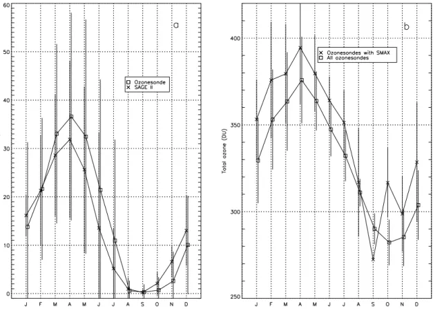
Fig. 4. (a) Secondary maxima monthly mean relative frequencies in Uccle ozone soundings and SAGE II ozone profiles in the latitude band 45-55N. (b) Total ozone column above Uccle for days with a secondary maximum and for all days with a sounding.
6 Frequency and seasonal cycle
Uccle ozone soundings were systematically scanned for sec-ondary maxima and we calculated the relative frequency of occurrence (RF) of secondary ozone maxima, that is, the fraction of ozone soundings at Uccle that showed a secondary ozone maximum. Figure 4a shows the monthly mean RF av-eraged over the period 1969–2001. Secondary maxima RF are higher during winter with a maximum in March-May, decrease sharply in June and July and fall to almost zero from August to November. This figure, in agreement with the findings of Mlch and Lavstovivcka (1996), is consistent with the scenario where laminae and secondary maxima ap-pear in conjunction with intense planetary wave activity and large disruptions of the polar vortex. The maximum RF oc-curs in March–April (Fig. 4a), which is the time of the year when the final breakdown of the northern polar vortex gener-ally occurs.
As the occurrence of secondary maxima is closely related to the state and position of the polar vortex, the occurrence of secondary maxima should also show some correlation with the total ozone column. It is clear from Fig. 4b that sec-ondary maxima RF are highly correlated with the total ozone seasonal cycle at Uccle. Figure 4b also shows that the to-tal ozone column is, in the average, higher than the
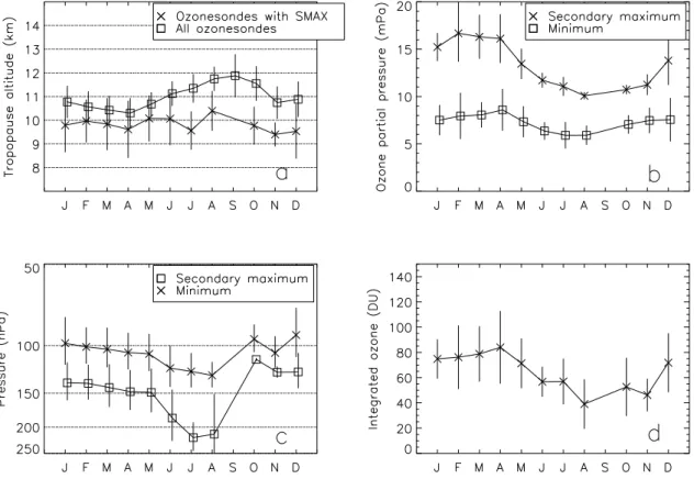
clima-tology by 20 DU when a secondary maximum is observed. This can be explained by the fact that the tropopause is gen-erally lower in or near the polar vortex than outside of it. And indeed, the observed average tropopause altitude for secondary ozone maxima events (Fig. 5a) is lower than the average tropopause altitude for all soundings by 1 to 2 km. It is interesting to note that there is almost no seasonal cy-cle in the tropopause height when a secondary ozone maxi-mum is observed while there is one in the mean tropopause height. Total ozone columns are higher even if the ozone minimum represents a loss compared to an undisturbed typi-cal vortex ozone profile. The integrated ozone value between the tropopause and the minimum (Fig. 5d) varies between 40 and 80 DU with large case-to-case variations.
The criterion to select secondary maxima uses relative dif-ferences between the secondary maximum and main maxi-mum and between the minimaxi-mum and secondary maximaxi-mum. Hence, there is no truncation at some threshold level and it makes sense to look at the absolute ozone concentration of the secondary maxima and its associated minima. Val-ues are shown in Fig. 5b. The ozone partial pressure at the secondary maximum has a well pronounced seasonal cycle while the partial pressure of the minimum shows little varia-tion over the year. The cycle of the secondary maximum par-tial pressure corresponds to the seasonal cycle of the lower
Fig. 5. (a) Monthly mean tropopause altitude for soundings with a secondary maximum and for all soundings. (b) Monthly mean ozone partial pressure of the secondary maxima and of the associated minima. (c) Monthly mean air pressure at the level of secondary maxima and associated minima. (d) Integrated ozone between the tropopause and the minimum concentration height. This graph gives the mean total ozone content of the secondary maximum. Error bars are one standard deviation on the mean. The period covered is 1969–2001.
stratospheric polar ozone, as ozone accumulates at the base of the polar vortex during winter, see Sect. 5. The partial pressure of the minimum is representative of lower strato-spheric low latitude air which undergoes little seasonal vari-ation. It is also clear from this figure that secondary maxima are more pronounced (larger ozone concentration difference between the minimum and the maximum) between Decem-ber and April than the rest of the year.
Ozone secondary maxima at Uccle occur typically around 140 to 160 hPa in winter and spring and below the 170 hPa level in summer (see Fig. 5c). This seasonal cycle is less pro-nounced in the corresponding curve of the associated min-ima. The minima typically occur around the 90 to 100 hPa level in winter and spring, with somewhat lower altitudes in summer. In this case, the larger pressure difference be-tween the minimum and the maximum occurs in summer and is smallest in October and November.
7 Zonal distribution
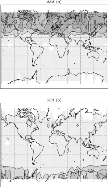
Using SAGE II ozone profiles, the zonal mean RF as well as the longitude/latitude distribution of secondary ozone max-ima can be investigated in much more detail than in previous studies. Of particular interest is the longitude/latitude
distri-bution shown in Fig. 6. The most striking features are the strong differences between the two hemispheres and the lat-itude gradient of the RF, with no ozone secondary maxima observed in the tropics and highest RF at high latitudes.
Appenzeller and Holton (1997) presented a climatology of lamination based on theoretical work and model calculation. They based their calculation on the size of the thermal wind shear derived from satellite temperature observations, and the size of ozone/tracer horizontal gradients. They showed that the production rate of ozone laminae has a dip between 30 and 10 hPa, likely because of the reversal of the ozone lati-tudinal gradient, and it then maximizes near 5 hPa. The zonal and seasonal distribution of secondary maxima observed by SAGE roughly agrees with the results by Appenzeller and Holton (1997) and the seasonal cycle of lamination in the lower stratosphere is also well described. However, substan-tial differences appear, especially in the southern hemisphere where the observations by SAGE exhibit a strong asymmetry between the southern and northern hemisphere which is not reproduced by Appenzeller and Holton (1997). Also, sec-ondary maxima RF steadily increase with increasing north-ern latitude except above westnorth-ern Europa and do not present a mid-latitude maximum found by (Appenzeller and Holton, 1997).
Fig. 6. Mean distributions of the percentage occurrence of ozone secondary maxima relative frequencies computed from SAGE II ozone profiles for (a) March to May and (b) September to Novem-ber. Areas where no data are available are white.
The origin of theses difference might be due to the differ-ent treatmdiffer-ent of laminae, as thin or weak lamina are excluded from the present study.
Ozone secondary maxima are not evenly distributes in lon-gitude, as expected from the observed association between secondary maxima and Rossby wave activity (Sect. 5). In the Northern hemisphere, secondary maxima appear prefer-entially in regions and at times where the atmospheric circu-lation is active, and planetary wave activity perturbs the polar vortex. Furthermore, the maximum RF in the north-eastern Atlantic, North Sea and Denmark seems to correspond to the eastern side of the northern Atlantic storm track (e.g. James, 1994).
The situation in the southern hemisphere is more com-plex as SAGE profiles measured in the ozone hole show low ozone values in the mid stratosphere, much like a secondary maximum. It is therefore very difficult to separate profiles showing a real dynamical secondary maximum, from ozone hole-type profiles where low ozone values in the lower strato-sphere are due to chemical depletion, at least at high lati-tudes. Nonetheless, it is clear that ozone secondary maxima occur much less frequently in the SH mid latitudes, (where no interference with the ozone hole is possible) than in the NH mid latitudes. The difference between the northern and southern hemisphere is likely due to the different circulation patterns in the mid latitudes, especially the much less fre-quent blocking systems in the southern hemisphere.
8 Trends in atmospheric circulation and ozone varia-tion
8.1 Trends in secondary maxima
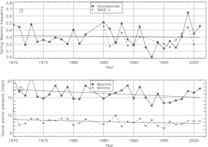
Figure 7a shows the time series of the mean February–May secondary maxima RF observed in Uccle ozone soundings and SAGE II profiles between 45circN and 55◦N latitude. Large year to year variations can be observed in both time series but with a reasonable correlation between Uccle and SAGE II even if SAGE II data are zonal mean values. There is no noticeable long term trend in the RF timeseries, in con-trast with the results of Mlch and Lavstovivcka (1996) who found pronounced negative trends in laminae occurrence at two central Europe sounding stations. The reason might again be in the exclusive consideration of large laminae in this study. Smaller laminae (included in the work by Mlch and Lavstovivcka (1996)) are confined to regions close to the polar vortex boundary so that their detection is extremely sensitive to the position of the polar vortex boundary. A small northward displacement of the vortex boundary will have a much greater impact on small laminae occurrence than on secondary maxima occurrence.
Figure 7b shows the mean February–May intensities of the ozone concentration of the secondary maxima and minima. Both show large year to year variations. A linear regression on the time series shows a significant negative trend for the secondary maximum intensity of −4.5%±2.2% per decade (1σ ), similar to the −5% per decade trend at 200 hPa at Res-olute (75◦N) for the period 1970–1996 (WMO, 1998).
Hood et al. (1999) and Steinbrecht et al. (2001) used one or several parameterizations of the atmospheric circulation in order to evaluate the contribution of the atmospheric cir-culation to decadal ozone trend in winter and spring month. In a similar exercise, following Fusco and Salby (1999) who showed that inter annual variation of total ozone operate co-herently with variations of planetary wave activity, it could be tried to use the RF of observed secondary ozone max-ima as a measure of the planetary wave activity at a given
Fig. 7. (a)Mean secondary maxima relative frequency in spring, from ozonesonde and SAGE II data. (b) Mean ozone partial pressure of the ozone secondary maxima and minima, from ozonesonde data.
location. We tried to relate this RF to the fluctuation of the total ozone column at the same location. This implies that the rate of ozone secondary maxima at a given station is rep-resentative of the frequency of maxima on a global scale. Al-though the zonal distribution is inhomogeneous (see Fig. 6), the RF of secondary maxima observed at Uccle compare rea-sonably well with the zonal mean values calculated from by SAGE II (see Figs. 4 and 7a).
The second parameter that can also be used to describe the atmospheric ozone content variability is the intensity of the secondary maxima. This value can be taken as a mea-sure of the lower polar vortex ozone concentration and can be expected to have an influence on the average lower strato-spheric ozone content as well as total ozone content down to mid latitudes. This is supported by the fact that most of the day-to day ozone variability comes from ozone variations in the lower stratosphere. It is important to note that any long term trend in ozone concentration due to chemical ozone de-pletion in the lower polar vortex could influence the intensity of secondary maxima.
8.2 Trends in ozone
A simple multiple linear regression model was used to de-scribe both the average total ozone content in spring above Uccle and the average ozone concentration in the lower stratosphere in spring above Uccle.
The ozone variability is described by O3(t )=C0t + C1SMAXF req(t )
+C2SMAXI nt ensity(t ) + C3SF (t ) (1)
where O3(t )is the ozone time series, C0is the fitted decadal
trend, SMAXF req(t )is the ozone secondary maxima relative
frequency, SMAXI nt ensity(t )is the ozone secondary
max-ima intensity time series, and SF (t ) is the solar flux variabil-ity.
This linear regression model was applied on the 30 years long time series of total ozone and lower stratospheric ozone concentration at Uccle. The total ozone timeseries is the mean total ozone column measured at Uccle by the Dobson instrument. All values are mean values for the month Febru-ary to May for each year.
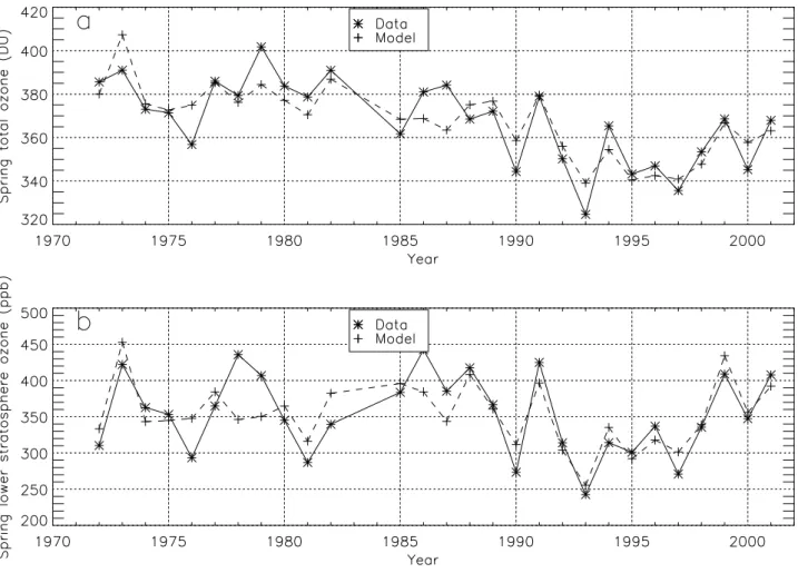
Fig. 8. (a) Mean spring Dobson total ozone at Uccle and results of the linear regression model. (b) Mean lower stratospheric spring ozone content at Uccle and result of the linear regression model.
The linear regression presented here includes a linear trend, the RF, and the intensity of ozone secondary max-ima measured at Uccle and the solar flux variability. This model is not intended to provide a complete description of the contributions to ozone variations. However, this model that simulates a simple linear trend and the influence of two dynamical parameters is able to account for 73% of the av-erage spring (February to April) total ozone variability. The correlation coefficient between the time series and the regres-sion model is R=0.86. The same model is able to account for 63% (R=0.79) of the lower stratospheric ozone concen-tration variability. The lower stratospheric ozone is taken to be the average ozone concentration between 11 and 13 km altitude. The results are shown in Fig. 8.
Looking at the spring lower stratospheric ozone concentra-tion first (Fig. 8b), we see that the model is able to reproduce a large part of the variability. The long term trend calculated with the model is −1.68%±2.38% per decade (1 sigma un-certainties). This value is not significant, even at the 68% confidence level. This figure can be compared to the value of −2.44% per decade obtained with a simple linear regression.
This means that the ozone variability and the observed long term ozone trend in the lowermost stratosphere can be de-scribed with the dynamical index given by SMAXF req and
a measurement of the lower polar vortex ozone concentra-tion given by SMAXI nt ensity. Since there is almost no long
term trend in the RF time series (Fig. 7a), this means that the trend in the lower stratospheric ozone concentration at Uccle is explained by trend in the polar lower stratosphere ozone content, represented here by SMAXI nt ensity.
The spring total ozone column variability (Fig. 8a), on the other hand, cannot be described by the parameteri-zation alone as the remaining trend given by the regression model is is −3.26%±0.67% per decade and is 2σ -significant. This trend can be explained by ozone depletion in the mid and upper stratosphere, at altitudes above those where ozone secondary maxima appear. Ozone depletion at mid-latitudes measured by ozonesondes shows significant negative trends that maximizes in the pressure range 200– 50 hPa (WMO, 2002), thus extending well above typical al-titudes of the phenomena studied here. Therefore, the trends in the middle and upper-stratosphere are not accounted for
by the parameterization used here. The remaining trend of −3.26%±0.67% is representative of the total ozone trend that is directly due to the effective reduction of ozone con-centration in the middle atmosphere at mid latitudes.
9 Conclusions
Thirty years of ozone soundings at Uccle and 15 years of SAGE II ozone profile data were analyzed to look for strong lamination events in the lower stratosphere called ozone sec-ondary maxima.
This study showed that:
– Ozone secondary maxima observed in ozone soundings
at Uccle occur often in conjunction with Rossby wave breaking events, mostly poleward backward and for-ward wave breaking events.
– Ozone secondary maxima are most frequent in spring
in both datasets and show a seasonal cycle that follows closely the total ozone seasonal cycle. Using SAGE II ozone profiles, the zonal distribution of secondary max-ima can be observed. This zonal distribution is not ho-mogeneous, with a correlation between the places of oc-currence of ozone secondary maxima and atmospheric circulation patterns.
– Using trajectory calculations, we found that secondary
ozone maxima are created through differential advec-tion in the lower stratosphere of ozone-rich air that comes from Northern high latitudes underneath ozone-poor air advected from close to the tropics. For the 17 cases studied, troposphere to stratosphere exchange as suggested by Dobson (1973) was not found and did not create the secondary maxima there.
– Year-to year variation of the mean relative frequency
of ozone secondary maxima as well as the variation of the mean intensity of the maxima can be used as an easily accessible measure of the atmospheric dynami-cal activity, or at least its component that has a direct influence on atmospheric ozone content variability. A multiple linear regression model using these two quan-tities can explain 73% of the mean February–April total ozone variability with a remaining trend of −3.26% per decade. The same model applied on the lower strato-spheric ozone content explains 63% of the variability with no significant remaining trend.
Acknowledgements. This work was supported by the EUMETSAT
Ozone Satellite Application Facility program. SAGE II ozone data are made available on-line by the NASA Langley Research Center (NASA-LaRC) and the NASA Langley Radiation and Aerosols Branch. The FLEXTRA trajectory model is made available by A. Stohl, Technical University of Munich.
Edited by: M. Dameris
References
Appenzeller, C. and Holton, J. R.: Tracer lamination in the strato-sphere: a global climatology, J. Geophys. Res., 102, 13 555– 13 569, 1997.
Danielsen, E., Hipskind, R. S., Starr, W., Vedder, J., Gaines, S., Kley, D., and Kelly, K.: Irreversible transport in the stratosphere by internal waves of short vertical wavelengths, J. Geophys. Res., 96, 17 433–17 452, 1991.
Dobson, G. M. B.: The laminated structure of the ozone in the at-mosphere, Q. J. R. Meteorol. Soc., 99, 599–607, 1973.
Fusco, A. and Salby, M.: Interannual variations of total ozone and their relationship to variations of planetary wave activity, J. Cli-mate, 12, 1619–1629, 1999.
Hood, L., Rossi, S., and Beulen, M.: Trend in lower stratospheric zonal winds, Rossby wave breaking behavior, and column ozone at northern midlatitudes, J. Geophys. Res., 104, D20, 24 321– 24 339, 1999.
James, I. N.: An introduction to circulating atmospheres, Cam-bridge University Press, 1994.
Mlch, P., and Lavstovivcka, J.: Analysis of laminated structures in ozone vertical profiles in central Europe, Ann. Geophys., 14, 744–752, 1996.
Lemoine, R. and De Backer, H.: Assesment of the Uccle ozone time series quality using SAGE II data, J. Geophys. Res., 106, 14 515–14 523, 2001.
Manney, G. L., Bird, J. C., Donovan, D. P., Duck, T. J., Whiteway, J. A., Pal, S. R., and Carswell, A. I.: Modeling ozone laminae in ground-based Arctic winter time observations using trajectory calculations and satellite data, J. Geophys. Res., 103, 5797–5814, 1998.
McCormick, M. P.: SAGE II: An overview, Adv. Space Res., 7, 3, 219–226, 1987.
O’Connor, F. M., Vaughan, G., and De Backer, H.: Observation of subtropical air in the European mid-latitude lower stratosphere, Q. J. R. Meteorol. Soc., 125, 2965–2986, 1999.
Peters, D. and Waugh, D. W.: Influence of barotropic shear in the poleward advection of upper-tropospheric air, J. Atmos. Sci., 53, 21, 3013–3031, 1996.
Plumb, R. A., Waugh, D. W., Atkinson, R. J., Newman, P. A., Lait, L. R., Schoeberl, M. R., Browell, E. V., Simmons, S. J., and Loewenstein, M.: Intrusions into the lower stratospheric Arctic polar vortex during the winter of 1991/1992, J. Geophys. Res., 94, 11 437–11 448, 1994.
Reid, S. J. and Vaughan, G.: Lamination in ozone profiles in the lower stratosphere, Q. J. R. Meteorol. Soc., 117, 825–844, 1991. Reid, S. J., and Vaughan, G.: Ozone laminae near the edge of the stratospheric polar vortex, J. Geophys. Res., 98, 8883–8890, 1993.
Reid, S. J., Vaughan, G., Mitchell, N. J., Prichard, I. T., Smit, J. H., Jorgensen, T. S., Varotsos, C., and De Backer, H.: Distribution of ozone laminae during EASOE and the possible influence of inertia-gravity waves, J. Geophys. Res., 21, 1479–1482, 1994. Steinbrecht, W., Claude, H., K¨ohler, U., and Winkler, P.:
Interan-nual changes of total ozone and northern hemisphere circulation patterns, J. Geophys. Res., 28, 7, 1191–1194, 2001.
Stohl, A.: A 1-year Lagrangian “climatology” of airstreams in the Northern Hemisphere troposphere and lowermost stratosphere, J. Geophys. Res., 106, 7263–7279, 2001.
Tuck, A. F., Davies, T., Hovde, S. J., Noguer-Alba, M., Fahey, D. W., Kawa, S. R., Kelly, K. K., Murpy, D. M., Proffitt, M. H., Margitan, J. J., Loewenstein, M., Podolske, J. R., Strahan, S. E., and Chan, K. R.: PSC-processed air and potential vorticity in the northern hemisphere lower stratosphere at mid-latitudes during winter, J. Geophys. Res., 97, 7883–7904, 1992.
Varotsos, C., Kalabokas, P., and Chronopoulos, G.: Association of the laminated vertical ozone structure with the lower strato-spheric circulation, J. Appl. Meteorol, 33, 473–476, 1994. Waugh, D. W., Plumb, R. A., Atkinson, R. J., Schoeberl, M. R.,
Lait, L. R., Newman, P. A., Loewenstein, M., Toohey, D. W., and Webster, C. R.: Transport out of the lower stratospheric Arctic vortex by Rossby Wave breaking, J. Geophys. Res., 99, 1071– 1088, 1994.
World Meteorological Organization (WMO): SAPRC/IOC/GAW Report No. 1, Assessment of trends in the vertical distribution of ozone, Ozone Research and Monitoring Project Report No. 43, 1998.
World Meteorological Organization (WMO): Scientific assessment of Ozone Depletion: 2002, Global Ozone Research and Monitor-ing Project Report No. 47, 2002.