A theoretical framework for trading experiments

HAL Id: halshs-00768898

https://halshs.archives-ouvertes.fr/halshs-00768898

Submitted on 26 Dec 2012

HAL is a multi-disciplinary open access

archive for the deposit and dissemination of

sci-entific research documents, whether they are

pub-lished or not. The documents may come from

teaching and research institutions in France or

abroad, or from public or private research centers.

L’archive ouverte pluridisciplinaire HAL, est

destinée au dépôt et à la diffusion de documents

scientifiques de niveau recherche, publiés ou non,

émanant des établissements d’enseignement et de

recherche français ou étrangers, des laboratoires

publics ou privés.

A theoretical framework for trading experiments

Maxence Soumare, Jørgen Vitting Andersen, Francis Bouchard, Alain Elkaim,

Dominique Guegan, Justin Leroux, Michel Miniconi, Lars Stentoft

To cite this version:

Maxence Soumare, Jørgen Vitting Andersen, Francis Bouchard, Alain Elkaim, Dominique Guegan, et

al.. A theoretical framework for trading experiments. 2012. �halshs-00768898�

A theoretical framework for trading experiments

Maxence

S

Jørgen Vitting A

Francis B

Alain E

Dominique G

Justin L

Michel M

, Lars S

A theoretical framework for trading experiments

Maxence Soumare1, Jørgen Vitting Andersen2,4, Francis Bouchard3, Alain Elkaim3, Dominique Gu´egan2, Justin Leroux3, Michel Miniconi1, and Lars Stentoft3

1

Laboratoire J.-A. Dieudonn´e Universit´e de Nice-Sophia Antipolis, Parc Valrose 06108 Nice Cedex 02, France

2

CNRS, Centre d’Economie de la Sorbonne, Universit´e Paris 1 Panth´eon-Sorbonne,

Maison des Sciences Economiques,

106-112 Boulevard de l’Hˆopital 75647 Paris Cedex 13 , France

3

HEC Montr´eal, 3000 chemin de la Cˆote Sainte-Catherine, Montr´eal, QC H3T 2A7, Canada

and

4

Corresponding author; email: [email protected], tel: +33 (0) 1 44 07 81 89; fax: +33 (0)1 44 07 81 18

∗

(Dated: November 21, 2012)

A general framework is suggested to describe human decision making in a certain class of experiments performed in a trading laboratory. We are in particular interested in discerning between two different moods, or states of the investors, corresponding to investors using fundamental investment strategies, technical analysis investment strategies respectively. Our framework accounts for two opposite situations already encountered in experimental setups: i) the rational expectations case, and ii) the case of pure speculation. We consider new experimental conditions which allow both elements to be present in the decision making process of the traders, thereby creating a dilemma in terms of investment strategy. Our theoretical framework allows us to predict the outcome of this type of trading experiments, depending on such variables as the number of people trading, the liquidity of the market, the amount of information used in technical analysis strategies, as well as the dividends attributed to an asset. We find that it is possible to give a qualitative prediction of trading behavior depending on a ratio that quantifies the fluctuations in the model.

Keywords: decision making, game theory, complex systems theory, technical analysis, rational expec-tations.

1. INTRODUCTION

In order to gain new insight on how investors perceive investment possibilities as well as risks in financial markets, it appears important to confirm not only the background of theoretical studies on human decision making, but also to get knowledge from controlled experiments, where one can probe in detail the different assumptions of investment behavior. It is only recently that experimental Finance has begun to appear as a well-established field, the interest in particular sparked by the recognition in terms of the attribution of the Nobel Prize in Economics to Vernon Smith in 2002. However, so far the major part of experimental work in Finance has assumed (Vernon Smith included) human rationality and the ability of markets to find the proper price close to an equilibrium setting. Contrary to this approach Behavioural Finance takes a more practitioner-minded description of how actual decision making takes place in financial markets. It would therefore seem like a very natural approach to bridge the insight gained from Behavioral Finance and apply it to experiments done on financial markets. Interestingly, not much effort has been done in this direction. The main reason is maybe because the major part of research done in Behavioural Finance is concerned with how individual decision making takes place (Prospect Theory included (Tversky and Kahneman (1974), Kahneman and Tversky (1979), and Tversky and Kahneman (1991) )) and in a

The efforts in this paper should be seen from such a viewpoint. Our theoretical foundation is based on a complex systems approach that places emphasis on social learning and group behaviour in order to understand the price formation in financial markets. The idea is that financial market participants are connected through their impact on the price as well as through the percolation of information through the group of market participants. For instance, “shocks” created by a large liquidation of a given market participant can have future impacts on the decision making of other market participants who in turn follow a similar decision to liquidate their positions. In the context where both dynamic behaviour as well as social learning and group behaviour are relevant, tools from complexity theory are particularly appealing, including for example agent-based modeling and game theory as presented here.

We are especially interested in discerning between two different moods (or states) of the population of investors, corresponding to i) investors using fundamental investment strategies as in the case of rational expectations and ii) the emergence of a speculative bias as seen in certain cases when investors use technical analysis strategies. The rational expectations case i) has been studied extensively in a large number of experiments under various situations and with different constraints (Smith (1962), Smith (1965), Plott and Smith (1978), Coppinger et al. (1980), Hommes et al. (2008)). In the simplest setup, which is included in our theoretical description further below, people trade shares of a given company based on their expectations of future dividends of the company. Throughout the experiment such expectations change due to the arrival of new information. The experiment ends with the closure of the company and the payout of the dividends to the participants in the experiments. It should be noted that in this case there is no incentive for the participants to speculate on the price itself since the full price of the company reflects the expected dividends payout at the end of the experiment. A case study was done for the opposite situation where expectations about dividends do not play any role, and reported in Roszczynska-Kurasinska et al. (2012). In this experiment only the price was available for the investment decisions of the group of participants. However as was shown in Roszczynska-Kurasinska et al. (2012) , it requires coordination among the participants to profit from a speculation bias in this kind of experiments.

It should be noted that our approach differs from most of the Behavioral Finance/bounded-rationality literature in that the phenomena we study can only be understood by looking at the system level. In other words, although the phenomena that emerge depend on microscopic features of the agents, it is important to not only look at individual characteristics but to study the system as a whole. The state of the system (speculative or fundamentalist) is the macroscopic result of many microscopic decisions. We shall refer to this collective “choice” of the state of the system as “aggregate decision making”.

Our setup is conducive to answering a number of well-defined questions–that of how prices form, for instance– that the Rational Expectations Hypothesis (REH), or even the bounded REH cannot address. Once one mixes in the two ingredients that are the asset price and the dividends, the situation becomes ambiguous: REH suggests agents should make their trading decisions based on dividends, but the matter becomes far from trivial once the price of an asset and an end date are factored in. Are decisions based on the price of the asset in anticipation of future price behavior (speculative state), or are dividends the only drivers of agents’ trading decisions (fundamentalist state)?

In the following we introduce theoretical foundations encompassing the occurrence of both the speculative and the fundamentalist state. We do so by considering the ”Dollar Game” (or ”$-Game”), which is an investment game that combines the two key ingredients that are dividends and the asset price (Vitting Andersen, Sornette (2003)) . Although simple in principle, the $-Game yields rich system dynamics, the complexity of which can be acted upon by the choice of system parameters (memory length, liquidity, etc.). As will be seen, this thereby creates a dilemma in terms of the investment strategies of the participants. The pure cases i) and ii) will appear as special cases of the general theory.

This feature of the $-Game lends itself well to study using a general well-known theory of phase-transitions found in Physics: the Ginzburg-Landau theory (henceforth referred to as ”the GL theory”) which we describe later.

2. THE $-GAME

The $-Game was inspired by the Minority Game (MG) introduced in 1997 by Ye-Cheng Zhang and Damien Challet (Challet and Zhang (1997), Challet and Zhang (1998) as an agent-based model proposed to study market price dynamics (Zhang (1998), Johnson et al. (1999), Lamper et al. (2002) ). The MG was introduced following a leading principle in Physics, that in order to solve a complex problem one should first identify essential factors

3 history, ~h(t) action, aj i(t) 000 1 001 -1 010 -1 011 1 100 -1 101 -1 110 1 111 -1 Example of a strategy

at the expense of trying to describe all aspects in detail. Similar to the Minority Game, the $-Game should be considered as a “minimal” model of a financial market.

Formally,N players (or agents) simultaneously take part in a one-asset financial market over a horizon of T periods. At each period,t ≤ T , each player i chooses an action ai(t) ∈ {−1, 1}, where action ”1” is interpreted

as ”buy” and action ”-1” as ”sell”. Players are assumed to be boundedly rational, in the sense of using only a limited information set upon which to base decisions. In the version of the $-Game presented in this paper, the agents use two different types of investment strategies, technical analysis strategies and fundamental analysis strategies. Concerning the decision making related to technical analysis, each player observes the history of past price movements, which is limited to the size of their memory,m ∈ N. Each player has at his/her disposal a fixed number ofs strategies which are randomly assigned at the beginning of the game. It follows that player i’s, j’th strategy,aj_i, is a mapping from the set of histories of sizem to {−1, 1}. We denote by ~h(t) ∈ {0, 1}m_{the history}

vector that agents observe in periodt before taking the action of either buying or selling an asset. We interpret ”1” to represent an up move of the market (an increase in the asset price) and ”0” corresponds to a down move of the market (a fall in the price of the asset). These assumptions are equivalent to having agents behave as technical analysts who use lookup tables to determine their next move. Table 1 shows an example of a strategy form = 3:

A strategy therefore tells an agent what to do given the past market behavior. If the market went down over the last three days, the strategy represented in Table 1 suggests that now is a good moment to buy (000 → 1) in Table 1. If instead the market went down over the last two days and then up today, the same strategy suggests that now is a good moment to sell (001 → −1) in Table 1. While a single strategy recommends an action for all possible histories (of lengthm), we also allow for agents to adopt different strategies over time. Namely, agents keep a record of the overall payoff each strategy would have yielded over the entire market history (i.e. not limited tom periods prior) and use this record to update which strategy is the most profitable. In every time period agenti therefore choses the best strategy (in terms of payoff, see definition below) out of the s available. This renders the game highly non-linear: as the price behavior of the market changes, the best strategy of a given agent changes, which then can lead to new changes in the price dynamics. The action of the best strategy of agent i at time t, is denoted by a∗

i(t). We denote by (a∗(t))i ∈ {−1, 1}N ×T the action profile of the population, where

~a∗_{(t) = (a}∗

1(t), ..., a∗N(t)) ∈ {−1, 1}N corresponds to the action played by theN agents in period t.

The payoffπ of the ith agent’s jth strategy, aji, in periodt is determined as follows:

π[aj_i] = aj_i(t − 1)

N

X

k=1

a∗k(t) (1)

The returnr(t) of the market between period t and t + 1 is assumed to be proportional to the order imbalance PN k=1a∗k(t): r(t) = N X k=1 a∗k(t)/λ (2)

withλ a parameter describing the liquidity of the market. Therefore the payoff of a given strategy (1) can be expressed in terms of the return of the market in the next time period as:

From (1) one can see that the payoff depends on two different times: the individual decision at timet − 1 and the aggregate ”decision” at timet. Such a feature of the payoff function is illustrative of real financial markets, where traders decide to enter a position in a market at timet − 1, but do not know their return until the market closes the next day (timet). This is especially clear from (3) where it can be seen that the $-Game rewards a given strategy that at timet − 1 predicted the proper direction of the return of the market r(t) in the next time step t. The larger the move of the market, the larger the gain/loss depending on whether the strategy properly/improperly predicted the market move. Therefore in the $-Game, agents correspond to speculators trying to profit from predicting the direction of price change.

In addition to technical analysis strategies that try to profit from price changes, we also consider strategies that try to profit from information of the fundamental value of an assetPf(t). Pf(t) is determined entirely from future

expectations about the dividendsd(t) attributed to the asset at the end of the experiment. Whenever P (t) > Pf(t) a

fundamental strategy therefore gives the recommendation to sell, whereas ifP (t) < Pf(t) it recommends buying.

Furthermore in order to take into account a diminishing use of such strategies in a purely speculative phase when the price P (t) >> Pf(t), the probability to use a fundamental strategy is taken from a Poisson distribution

γ exp (−γ) with γ =P (t)−Pf

d .

To sum up, the $-Game as described in this article can be described in terms of just five parameters: • N - The number of agents (market participants).

• m - The memory length used by the agents.

• s - The number of strategies held by the agents. It should be noted that the s strategies of each agent is chosen randomly (corresponding to a random column of ‘0’s and 1’s in table 1) in the total pool of 22m

strategies at the beginning of the game. • λ - The liquidity parameter of the market.

• d(t) - The future expectations about the dividends paid at the end of the experiment. To simplify, d(t) will be taken constant in timet in this paper.

The dynamics of the $-Game are driven by nonlinear feedback because each agent uses his/her best strategy at every time step. As the market changes, the best strategies of the agents change, and as the strategies of the agents change, they thereby change the market. Formally one can understand such dynamics by representing the price historyh(t) =Pm_j=1b(t − j + 1)2j−1_{as a scalar whereb(t) is the bit representing the direction of price movement}

at timet (see table 1). The dynamics of the $-Game can then be expressed in terms of an equation that describes the dynamics ofb(t) as:

b(t + 1) = Θ(

N

X

i=1

a∗i(h(t))), (4)

withΘ a Heaviside function. The nonlinearity of the game can be formally seen from:

a∗i(h(t)) = a {j|maxj=1,...,s{Π[aji(h(t))]} i (h(t)), Π[a j i(h(t))] = t X k=1 aji(h(k − 1)) N X i=1 a∗i(h(k)) (5)

Inserting the expressions (5) in expression (4) one obtains an expression that describes the $-Game in terms of just one single equation forb(t) depending on the values of the variables (m, s, N, λ, d) and the random variables aj_i (i.e. their initial random assignments). A major complication in the study of this equation happens because of the non-linearity in the selection of the best strategy. Fors = 2 however the expressions simplifies because one only need to know the relative payoffqi ≡ π[a1i] − π[a2i] between two strategies (Challet, Marsili (1999),

Challet, Marsili (2001) ). For this special case it was shown in Roszczynska-Kurasinska et al. (2012) that the Nash equilibrium for the $-Game with only technical analysis strategies (with no cash nor asset constraints) is akin to that of Keynes’ “Beauty Contest” where it becomes profitable for the subjects to guess the actions of the other participants. The optimal state is then one for which all subjects cooperate and take the same decision (either buy/sell).

5

3. GINZBURG-LANDAU THEORY

To describe further the competition between technical analysis trading strategies and fundamental analysis trad-ing strategies as used in the $-Game, we suggest to borrow a description from Physics where different states of a system can be characterized via a so-called free energyF . F in that case plays a central role, since its minimum determines how the state of the system will appear. F can be written as F = E − T S with E the energy of the system,T the temperature and S the entropy which one can think of as representing how much disorder there is in a given system. From the definition ofF we can see that the state of a system is determined by a struggle between two different forces, one representing “order”, this is theE term, and the other term representing “disorder” given by theT S term. We suggest a similar struggle of “forces” to be present in the trading experiments.

The competition between order and disorder as described byF , can be understood in more detail by considering the example given by the Ising model, which is a model of ferromagnetism. For the Ising model the energy E = −JP<i,j>sisjwithsi, sjrepresenting the atomic “spins” of a material. The<>-notation in the summation

indicates that the sum is to be taken over all nearest neighbors pair of spins. Each spin itself can be thought of as a mini magnet. In the two-dimensional Ising model the spinsi = 1 if the spin is “up” and si = −1 if the spin

is “down”. Taking the coupling strength between spinsJ positive, the minimum energy Emin of the system is

simply given by either all spins up(si ≡ 1), or all spins down (si ≡ −1). For temperature T = 0 the minimum

of the energyE is therefore also the minimum of the free energy F . However as soon as T > 0, the finite temperature will introduce fluctuations of the spins introducing thereby a non-zero contribution to the entropyS. The larger the temperatureT the larger this tendency, until at a certain temperature Tc above which order has

completely disappeared - the system is in a disordered state. Order in the case of the Ising model is measured by the magnetism, which is just the averaged value of the spinm = E(si).

GL theory introduces the idea that we can in general understand such order-disorder transitions mentioned above by expanding the free energy in terms of the order parameterm. Specifically write:

F = C + am + αm2+ bm3+ β/2m4+ ... (6)

Using now the symmetry argument that there should be no difference in the free energy between the two states with respectively either allsi ≡ 1 or si ≡ −1, all odd order terms in m disappear in (6). Taking furthermore the

derivative (in order to find its extreme) we end up with the equation at a minimum ofF :

0 = m(α + βm2_{) (7)}

(7) has the trivial solution of the magnetizationm = 0, this is the high temperature solution and describe the disordered state. Takingβ positive, the other non-trivial solution happens for negative α, m2_{= −α/β. By writing}

α = (T − TC) one sees that the magnetization scales as (T − T c)1/2for temperatures belowTc. The exponent of

0.5 is the so called “mean field” or GL exponent of the transition.

We now propose to consider in similar terms the competition in the trading experiments between profit from speculation obtained through trend-following, versus the tendency to destroy such trends due to mean reversion towards the fundamental price (Vitting Andersen (2010). The general tendency to create either a positive/negative price trend corresponds to “order” whereas either the lack of consensus or the mean reversion to the fundamental price value will destroy such order. To make the analogy with our discussion above, we introduce what one could call the “free profit” given by two termsFP = P − T S. P is the profit of the ordered state which for T = 0

corresponds to a continuous up/down trend of the market.S is an entropy term that destroys the ordered state, and T is the “temperature” which will be introduced below.

As discussed beforehand, the payoff of a strategy in the $-Game describes the profit for the given strategy. Agents in a Nash equilibrium are characterized by using the same strategy over time, therefore such a strategy has to be optimal. We can then write the total profitP for the system of traders in a Nash equilibrium of the $-Game as: P (t) = X i π[a∗i] (8) = N X i=1 N X j=1 a∗i(t − 1)a∗j(t) (9)

We note the resemblance of (9) to the Ising model described above. One major difference with respect to the Ising model however is the “interaction” between traders, since (9) says that traderj’s action at time t has an impact on traderi’s profit from the action he/she took at time t − 1. Therefore the “interaction” is seen to be “long-ranged” in (9) whereas the interaction is local (it only concerns nearest-neighbors) for the Ising model.

Similar to (6) we can introduce an order parameter and expand the “free profit” in terms of this parameter. In the case of the Ising model the order parameter is given by the spatial average of the local order (the magnetization). In the trading setup we suggest to consider the local order o expressed in terms of the order imbalance: o = 1/NPNi=1a∗i which from (2) is seen to be proportional to the return. The parametero varies between -1 (all

agents decide to sell) and 1 (all agents decide to buy). In the case where one can neglect the dividends (the experiment described in Roszczynska-Kurasinska et al. (2012)o → ±1 so this corresponds to the complete ordered outcome. For the experiments performed under the assumptions of rational expectations the price converges to the fundamental price in the end of the experiments and we geto → 0 for t → tn with tn the duration of the

experiment.

Applying now the GL idea and expandingFp in terms of o, one ends up with the very same conditions (7)

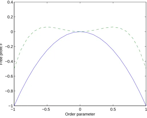
to determineo, except that the extreme (extremes) now describes a maximum (maxima) instead of a minimum (minima) as was the case forF . Note that all odd order terms of o disappear since there is no difference in the profit that traders obtain in shorting the market compared to going long. Figure 1 illustrates the expansion ofFp

(y-axis) as a function of o (x-axis) for the two cases: i) the T > Tcsolution (i.e. the disordered state corresponding

to no trend in the experimentso = 0) can be seen as the maximum of the solid line, whereas the two T < Tc

solutions (i.e. the ordered state corresponding to a certain trend in the experimentso 6= 0) can be found as the maxima of the dashed line.

One of the main implications of the GL theory is the existence of a nontrivial transition from a high “tempera-ture” disordered state in the trading experiments where traders don’t create a trend over time, to a low ‘tempera“tempera-ture” state characterized by trend following. A “temperature” can now be defined via the randomness of the model as will be explained in the following. Randomness enters the $-Game through the initial conditions in the assignments of thes strategies to the N traders in the game. In order to create a given strategy one has to assign randomly either a0 or a 1 for each of the 2m_{different price histories. Therefore the total pool of strategies increases as2}2m

versus m. However many of these strategies are closely related - take e.g. table 1 and change just one of the 0’s to a 1, this thereby creates a strategy which is highly correlated to the one seen in table 1. In Challet, Zhang (1997), Challet, Zhang (1998), it was shown how to construct a small subset of size2m_{of independent strategies out of}

the total pool of22m

strategies. As suggested in (Savit et al. (1999) and Challet, Marsili (2000)) , a qualitative understanding of the MG can then be obtained by considering the parameterα ≡ 2m

N . However as pointed out in

Zhang (1998) the ratioα′ = _{N ×s}2m seems intuitively to be more relevant since this quantity describes ratio of the total number of relevant strategies to the total number of strategies held by the traders. Taking into account the presence of a fundamental value strategy we therefore introduce the ratioT = 2_{N ×s}m+1 to describe the temperature in the simulations of the $-Game presented in the following. The relation ofT to the fluctuations of the system becomes clear when one consider that when sampling the variance of a small sample is larger than the variance of a large sample (a fact called “the law of small numbers” in Psychology/Behavioral Finance (Tversky, Kahneman (1974), Kahneman, Tversky (1979), Tversky, Kahneman (1991) ). Therefore when the sample of strategies held by theN traders is small with respect to the total pool of relevant strategies, this corresponds to the large fluctuations, large temperature case. Vice versa a large sample of strategies held by theN traders therefore corresponds to a small temperature case as seen from the definition ofT .

4. RESULTS

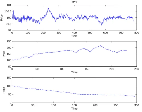
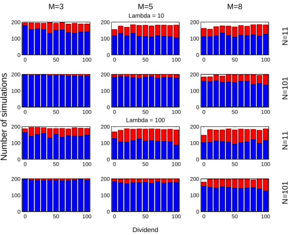
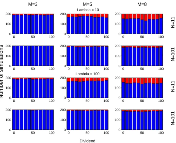
Figure 2 shows three different results representing typical market behavior corresponding to fundamental price behavior, as well as speculative behavior in an increasing/decreasing market. Figure 3-4 show histograms rep-resenting respectively speculative behavior (blue) or fundamentalist behavior (red) as outcomes in a setup of the $-Game corresponding to a trading experiment with given realizations of the 5 parameters(N, m, s, λ, d). The histograms in figure 2 represents simulations performed withs = 2 whereas the histograms in figure 3 were done for simulations withs = 18. The different histograms were obtained from an ensemble average of 200 simulations of the $-Game where each realization of the game were run for up to200 ∗ 2m_{time steps. A speculative state was}

7

the price fluctuation within a 50 percentage range of the fundamental valuePf. White in the figures represents the

cases where neither a definite speculative nor fundamental state could be defined.

We first notice the somewhat surprising fact that the dividendsd as well as the liquidity of the market λ, only seem to have a quite limited impact on the final state of the market. In particular for the smallestm values (m = 3, 5) increasing dividends appear to have a somewhat stabilizing effect allowing for slightly more fundamental value states. The same stabilizing trend appears to be at play as one increases the liquidity of the market, but again, this tendency appear to be very weak. A much clearer tendency is seen with respect to increasing speculation when increasing the number of tradersN , respectively decreasing the amount of information m used in the decision making of the technical analysis trading strategies. A larger number of strategiess assigned to the traders is also seen to enhance speculation (compare figure 3 and figure 4).

One of our main results is that a qualitative behavior of a trading experiment can be predicted depending on the given value ofT . In particular with respect to expectations about the outcome in an experimental setup of the market model, such an understanding is important (Bouchard et al. 2012). The fact thatT determines the outcome of trading behavior can be seen by changing the nominator and denominator by the same factor, which then should lead to invariant behavior in terms of trading decisions. This means that for example the(m = 3, N = 11) (i.e. T = 0.72/s) trading behavior for a given λ and s should fall in between the (m = 5, N = 101) (i.e. T = 0.32/s) and(m = 8, N = 101) (i.e. T = 1.27/s) cases. From figure 2 and figure 3 this is seen indeed to be the case. Similarly comparing figure 3-4 it is seen that increasing (/decreasing)N and decreasing (/increasing) s by the same amount leads to two systems behaving similarly in terms of investment profile (compareN = 101 rows in figure 3 toN = 11 rows in figure 4) . These results underscore the importance of the parameter T when it comes to the understanding of the aggregate decision making in the model.

5. CONCLUSION

A general framework has been suggested to describe the human decision making in a certain class of experi-ments performed in a trading laboratory. Our framework allows us to predict the outcome of such type of trading experiments in terms of when to expect a fundamental versus a speculative state. We have shown how a qualitative understanding could be found depending on just one parameter, representing the fluctuations of the model. Our findings give certain guidance with respect to the implementation of trading experiments performed in a trading laboratory (Bouchard et al. (2012)).

6. ACKNOWLEDGMENTS

J.V.A., M. M. and M. S. would like to thank the Coll`ege Interdisciplinaire de la Finance for financial support.

∗ _{Electronic address:[email protected]}

F. Bouchard et al. forthcoming (2012)

Challet D., Zhang Y.-C., 1997. Emergence of cooperation and organization in an evolutionary game. Physica A 246, 407-418

Challet D., Zhang Y.-C., 1998. On the Minority Game: Analytical and numerical studies. Physica A 256, 514 Challet D., Marsili M., 1999. Physical Review E 60, R6271

Challet D., Marsili M., 2000. Physical Review E 62, 1862

Coppinger V. M., Smith V. L, Titus J. A., 1980. Incentives and behavior in English, Dutch and sealed-bid auctions. Economic Inquiry 18, 1-22

Hommes C., Sonnemans J., Tuinstra J., van de Velden H., July 2008. Expectations and bubbles in asset pricing experiments. Journal of Economic Behavior & Organization, 67(1) 116-133 ISSN 01672681. doi: 10.1016/j.jebo.2007.06.006.

Johnson N. F., Hart M., Hui P., 1999. Crowd effects and volatility in markets with competing agents. Physica A 269, 1-8 Kahneman D., Tversky A., 1979. Prospect theory: an analysis of decision under risk. Econometrica 47, 263-291

Lamper D., Howison S. D., Johnson N. F., 2002. Predictability of large future changes in a competitive evolving population. Physical Review Letters 88, 017902

Marsili M., Challet D., 2001. Physical Review E 64, 056138-1

Plott C., Smith V. L., 1978. An experimental examination of two exchange institutions. Review of Economic Studies 45, 133-153

Roszczynska-Kurasinska M, Nowak A., Kamieniarz D., Solomon S., Andersen J. V., 2012. Short and long term investor synchronization caused by decoupling. In press 2012, PLoSONE

Savit R., Manuca R., Riolo R., 1999. Physical Review Letters 82, 2203

Smith V. L., 1962. An experimental study of competitive market behavior. Journal of Political Economy 70, 111-137 Smith V. L., 1965. Experimental auction markets and the Walrasian hypothesis. Journal of Political Economy 73, 387-393 Tversky A., Kahneman D., 1974. Judgment under uncertainty: heuristics and biases. Science 185, 1124-1131

Tversky A., Kahneman D., 1991.Loss aversion in riskless choice: A reference-dependent model. Quarterly Journal of Economics 106, 1039-1061

Vitting Andersen J., 2010. Detecting anchoring in financial markets. Journal of Behavioral Finance 11, 2, 129-33 Vitting Andersen J., Sornette D., 2003. The $-game. European Physics Journal B 31, 141-145

9 −1 −0.5 0 0.5 1 −1 −0.8 −0.6 −0.4 −0.2 0 0.2 0.4 Order parameter Free profit F

FIG. 1: Illustration of the “Free Profit” Fpas a function of the order parameter o for two different “temperuatures”

0 100 200 300 400 500 600 700 800 99 99.5 100 100.5 101 M=5 Time Price 0 50 100 150 200 250 50 100 150 200 250 Time Price 0 50 100 150 200 250 300 0 50 100 150 Time Price

11 0 50 100 0 100 200 M=3 0 50 100 0 100 200 M=5 Lambda = 10 0 50 100 0 100 200 M=8 N=11 0 50 100 0 100 200 0 50 100 0 100 200 0 50 100 0 100 200 N=101 0 50 100 0 100 200

Number of simulations

FIG. 3: Histograms representing respectively speculative behavior (blue) or fundamentalst behavior (red) as outcomes in a

0 50 100 0 100 200 M=3 0 50 100 0 100 200 M=5 Lambda = 10 0 50 100 0 100 200 M=8 N=11 0 50 100 0 100 200 0 50 100 0 100 200 0 50 100 0 100 200 N=101 0 50 100 0 100 200

Number of simulations

FIG. 4: Histograms representing respectively speculative behavior (blue) or fundamentalst behavior (red) as outcomes in a