HAL Id: tel-01677857
https://tel.archives-ouvertes.fr/tel-01677857
Submitted on 8 Jan 2018HAL is a multi-disciplinary open access archive for the deposit and dissemination of sci-entific research documents, whether they are pub-lished or not. The documents may come from teaching and research institutions in France or abroad, or from public or private research centers.
L’archive ouverte pluridisciplinaire HAL, est destinée au dépôt et à la diffusion de documents scientifiques de niveau recherche, publiés ou non, émanant des établissements d’enseignement et de recherche français ou étrangers, des laboratoires publics ou privés.
Decision diagrams : constraints and algorithms
Guillaume Perez
To cite this version:
Guillaume Perez. Decision diagrams : constraints and algorithms. Other [cs.OH]. Université Côte d’Azur, 2017. English. �NNT : 2017AZUR4081�. �tel-01677857�
UNIVERSITÉ COTE D’AZUR
Doctoral thesis
Decision Diagrams: Constraints and Algorithms
Defended by
Guillaume Perez
to obtain the title of
Doctor of Science
Specialty : Artificial Intelligence
Thesis Advisor: Jean-Charles Régin
prepared at I3S Sophia Antipolis, MDSC Team Doctoral School STIC
defended on September 29, 2017
Jury :
Reviewers : Roland Yap - National University of Singapore
Nicolas Beldiceanu - IMT Atlantique
Willem-Jan van Hoeve - Carnegie Mellon University
President : David Coudert - INRIA Sophia Antipolis
Examinators : Pierre Schaus - Université Catholique de Louvain
François Pachet - Sony CSL
Michel Barlaud - Université Nice - Sophia Antipolis Arnaud Malapert - Université Nice - Sophia Antipolis Advisor : Jean-Charles Régin - Université Nice - Sophia Antipolis
Abstract
Multivalued Decision Diagrams (MDDs) are efficient data structures widely used in several fields like verification, optimization and dynamic programming. In this thesis, we first focus on improving the main algorithms such as the re-duction, allowing MDDs to potentially exponentially compress set of tuples, or the combination of MDDs such as the intersection of the union. We go further by designing parallel algorithms, and algorithms handling non-deterministic MDDs. We then investigate relaxed MDDs, that are more and more used in optimization, and define the notions of relaxed reduction or operation and de-sign efficient algorithms for them. The sampling of solutions stored in a MDD is solved with respect to probability mass functions or Markov chains. In order to combine MDDs with constraint Programming, we design the propagators of all the types of MMDD constraints in solvers, and introduce a new one, the channeling constraint. These new propagators outperform the existing ones and allow the reformulation of several other constraints such as the dispersion constraint, and even to define new ones easily. We finally apply our algorithm to several real world industrial problems such as text and music generation and geomodeling of a petroleum reservoir.
ii
Résumé
Les diagrammes de décision Multi-valués (MDD) sont des structures de don-nées efficaces et largement utilisées dans les domaines tels que la vérifica-tion, l’optimisation et la programmation dynamique. Dans cette thèse, nous commençons par améliorer les principaux algorithmes tels que la réduction de MDD, permettant aux MDD de potentiellement compresser exponentiel-lement des ensembles de tuples, ou la combinaison de MDD, tels que l’in-tersection ou l’union. Ensuite, nous proposons des versions parallèles de ces algorithmes ainsi que des versions permettant de travailler avec la version non déterministe des MDD. De plus, dans le domaine des MDD relâchés, un domaine de plus en plus étudié, nous définition les notions de réduction et combinaison relâchés, ainsi que leurs algorithmes associés. Nous résolvons le problème de l’échantillonnage des solutions d’un MDD avec respect de loi de probabilité tels que des fonctions de probabilité de masse ou des chaines de Markov. Pour permettre d’utiliser les MDD dans les solveurs de programma-tion par contraintes, nous proposons de nouveaux propagateurs pour toutes les contraintes basées sur des MDD, améliorant les performances des algorithmes existants, puis nous en introduisons une nouvelle contrainte, la contrainte de channeling. Grâce à eux, nous montrons que nous pouvons reformuler plu-sieurs contraintes et en définir de nouvelles tout en étant basés sur des MDD. Finalement nous appliquons nos algorithmes à des problèmes industriels réels de génération de texte et musique, et de modélisation de réservoir de pétrole.
iii
Acknowledgments
I would like to thank my advisor Prof. Jean-Charles Régin. For having bet on me even years before my PhD, and for all his useful advices and encourage-ments during this thesis. Jean-Charles is one of the most intelligent person I had the opportunity to met in my life, and its ability to constantly share its knowledge is wonderful.
Many works inside of this PhD could have never existed without several researchers and the great collaborations we had. I would like to thanks them all. First Laurent Perron, at the beginning of my PhD. Then François Pachet, Pierre Roy and Alexandre Papadopoulos, which have provided me many good advices and insights on many fields. Also, I had the chance to work with Pierre Schaus and Christophe Lecoutre, which have provided me a great view of real world problems.
Inside of my laboratory, I had the luck to work with Michel Barlaud and Lionel Fillatre. I particularly want to thank them, for their patience and for having provided me so much useful knowledge on mathematical optimization. I am happy to thank Arnaud Malapert, for its many useful comments con-stantly allowing me to take a step back on most of my works, and for the work we have already done together, or for the next coming. I would like to thanks the many people in my lab, for the right working environment and the great atmosphere they have provided me. So thank you Sandra Devauchelle, Enrico Formenti, Benjamin Miraglio, Jonathan Behaegel, Ophelie Guinaudeau, and the many others.
I have a lot of gratitude for my friends. First, Mehdi Ahizoune, my best friend, and Yoan Kraria, Nicolas Huin, Anthony Palrmieri, Heytem Zitoun, Yassine Ferkouch, Jean-Michel Diaz Vaz, Sami (y) Lazreg. I thank them for the support they have provided me these last years.
I have a big thank for my family, for my mom Veronique, my brother and sisters, Virginie, Yannick and Doreenda. I would not be without them; they are my models for so many reasons. I would also thanks my step-parents, Isabelle and Jean, for their wonderful support.
Finally, and the most important, I would like to thank my Wife, Marion. She is my principal inspirational source. She has supported me, motivated me and encouraged me all along these years.
Contents
1 Introduction 1
1.1 Introduction and Motivation . . . 1
1.2 Contributions and Outline . . . 9
1.2.1 Inside this thesis . . . 9
1.2.2 Other Contributions . . . 11
2 Definitions & Related Work 13 2.1 Definitions and Notations . . . 13
2.1.1 Constraint Programming . . . 13
2.1.2 Multi-valued Decision Diagrams . . . 14
2.2 Related Work . . . 16 2.2.1 Automaton . . . 19
I
MDDs: Fundamental Algorithms
23
3 Reduction 25 3.1 Introduction . . . 25 3.2 Related Work . . . 273.3 pReduce, a linear reduction operator . . . 30
3.3.1 ipReduce, Incremental reduction. . . 33
3.4 Experiments . . . 37
4 Constructions 41 4.1 Introduction . . . 41
4.2 Table and Trie. . . 43
4.2.1 Trie . . . 43
4.2.2 Table. . . 43
4.2.3 Linear table transformation . . . 45
4.3 Global Cut Seed and Tuple Sequences. . . 47
4.3.1 Definitions . . . 47
4.3.2 Transformations . . . 48
4.4 Automaton . . . 51
4.4.1 Definition and related work . . . 51
4.4.2 New method. . . 53
4.5 Experiments . . . 54
4.5.1 Table. . . 54
vi Contents 5 Operations 59 5.1 Related Works. . . 60 5.1.1 BDD Apply . . . 60 5.1.2 BDD to MDD . . . 64 5.2 Graph-Based Apply . . . 66 5.2.1 Graph-Based Algorithm . . . 68
5.2.2 Avoiding Data structures . . . 72
5.3 In-place Operations . . . 76
5.3.1 Deletion of tuples from an MDD. . . 78
5.3.2 Addition of tuples to an MDD . . . 79 5.4 Experiments . . . 84
II
MDDs: Advanced Algorithms
87
6 Parallel Computing 89 6.1 Introduction . . . 89 6.1.1 Related Work . . . 90 6.2 Background . . . 90 6.2.1 Parallelism. . . 90 6.3 Parallel Reduction . . . 91 6.3.1 Parallel Sort . . . 92 6.3.2 Parallel pReduce . . . 94 6.3.3 Discussion . . . 97 6.4 Parallel Apply . . . 98 6.5 Experiments . . . 100 6.6 Conclusion . . . 103 7 Non-deterministic operation 105 7.1 Introduction . . . 1057.2 Apply for Non Deterministic . . . 107
7.3 Apply for Deterministic . . . 108
8 Relaxations 113 8.1 Introduction . . . 113
8.2 Relaxed Creation : Existing Works . . . 115
8.3 Relaxed Creation : New Method. . . 116
8.3.1 Delayed Relax Creation . . . 116
8.3.2 Generalization . . . 117
8.3.3 Generic merging heuristic . . . 118
8.3.4 States relaxation . . . 118
Contents vii 8.5 Relaxed Combination . . . 119 8.5.1 Relax Apply . . . 120 8.5.2 Experiments . . . 123 8.6 Relaxed MDDs : Use . . . 124 9 Sampling 127 9.1 Introduction . . . 127 9.2 Definitions . . . 129 9.2.1 Probability distribution . . . 129 9.2.2 Markov chain . . . 130 9.3 Sampling and MDD . . . 131
9.3.1 PMF and Independent variables . . . 131
9.3.2 Markov chain . . . 134
9.3.3 Incremental modifications. . . 139
9.4 Experiments . . . 139
9.4.1 PMF constraint and sampling . . . 140
9.4.2 Markov chain and sampling . . . 141
9.4.3 Big Number generation . . . 142
9.5 Conclusion . . . 142
III
MDDs: Constraints and Propagators
145
10 Table & MDD-based Constraints 147 10.1 Introduction . . . 14710.2 Related Work . . . 150
10.2.1 Table Constraint propagators . . . 150
10.2.2 MDD Constraint Propagators . . . 154
10.2.3 Sparse Set . . . 165
10.3 GAC-4R: Table Propagator . . . 166
10.3.1 GAC-4 . . . 166 10.3.2 GAC-4R . . . 167 10.4 MDD4R: MDD Propagator. . . 170 10.4.1 MDD4 Algorithm . . . 170 10.4.2 MDD-4R. . . 173 10.4.3 Improvements . . . 175 10.5 Experiments . . . 178 10.5.1 CP14 experiments . . . 179 10.6 Conclusion . . . 180
viii Contents 11 Cost-MDD constraint 183 11.1 Introduction . . . 183 11.2 Cost-MDD . . . 185 11.2.1 Definition . . . 185 11.2.2 Related Work . . . 186 11.3 Cost-MDD4R . . . 188 11.3.1 Variable Modification . . . 188
11.3.2 Modification of the cost value. . . 192
11.4 Cost Intersection Method. . . 194
11.4.1 Discussion . . . 197 11.5 Experiments . . . 198 11.5.1 MaxOrder . . . 198 11.5.2 Random instances. . . 198 12 Soft-MDD constraint 199 12.1 Introduction . . . 199 12.2 Soft-MDD Propagator . . . 200 12.2.1 Dedicated Propagator . . . 202
12.2.2 Transformation into a cost-MDD . . . 203
12.2.3 Intersection of MDDs . . . 203
12.3 Discussion . . . 204
12.4 Experiments . . . 206
13 Channeling Constraints and MDDs 209 13.1 Introduction . . . 209 13.2 MDD Channeling Constraint . . . 211 13.2.1 Set Variables . . . 211 13.2.2 Definition . . . 211 13.3 Propagation . . . 212 13.3.1 Modification of I . . . 212 13.3.2 Modification of V . . . 213 13.3.3 Modification of the MDD . . . 216 13.4 Conclusion . . . 219
IV
MDDs: Constraints Modeling
221
14 Allen constraint 223 14.1 Introduction and Related Works . . . 22314.2 Constraining Contiguous Temporal Sequences . . . 225
14.2.1 Definition of the Allen Constraint . . . 226
Contents ix
14.3.1 A First Model . . . 227
14.3.2 MDD-Based Model . . . 229
14.4 Experiments . . . 232
14.4.1 Evaluation of the First Model . . . 232
14.4.2 Evaluation of the MDD-Based Model . . . 233
14.5 Conclusion . . . 233
15 Markov and Statistical Constraints 235 15.1 Introduction . . . 235
15.2 Definition . . . 237
15.2.1 Probability distribution . . . 237
15.2.2 Markov chain . . . 237
15.2.3 MDD of a Generic Sum Constraint . . . 238
15.2.4 Dispersion Constraint. . . 239
15.3 Dispersion Constraint . . . 239
15.3.1 Dispersion Constraint with fixed mean . . . 239
15.3.2 Dispersion Constraint with variable mean . . . 240
15.4 Probabilities Based Constraint . . . 241
15.4.1 MDDs and Probabilities based constraints . . . 241
15.4.2 Probabilities and Means . . . 242
15.5 Experiments . . . 243 15.6 Conclusion . . . 245 16 Unefficient MDDs 247 16.1 Introduction . . . 247 16.2 AllDifferent . . . 247 16.3 Set Variables . . . 248 16.4 Pareto . . . 249
16.4.1 Storing the Pareto solutions . . . 249
16.4.2 Pareto Constraint . . . 250
16.4.3 MDD as a store for the Pareto set . . . 250
16.4.4 Why does this Fail?. . . 253
16.5 Conclusion . . . 253
V
Applications
255
17 MaxOrder 257 17.1 Introduction . . . 257 17.2 Models . . . 258 17.2.1 Model 1 . . . 258 17.2.2 Model 2 . . . 259x Contents
17.2.3 Model 3 . . . 260
17.2.4 Experiments . . . 262
17.3 Soft Version . . . 265
17.3.1 Introduction and Model . . . 265
17.3.2 Experiments . . . 266
17.4 Conclusion . . . 266
18 Audio Multitrack Synchronization 269 18.1 Introduction . . . 269
18.2 Description of the Benchmark . . . 270
18.3 Experiments . . . 273
18.3.1 First Allen Model . . . 273
18.3.2 MDD-Based Allen Model. . . 273
19 Geomodeling of a Petroleum reservoir 275 19.1 Introduction . . . 275 19.2 Models . . . 276 19.2.1 Problem . . . 276 19.2.2 Results . . . 277 19.3 Conclusion . . . 278 20 Conclusion 279 20.1 Conclusion . . . 279 20.2 Perspectives . . . 280
VI
Appendix
281
A Implementation 283 A.1 Array Implementation . . . 283A.2 List Implementation . . . 289
A.2.1 Conclusion . . . 295
B Algorithms and Data Structures 297 B.1 Sorting . . . 297
B.1.1 Indexing sort . . . 297
B.1.2 Counting sort . . . 298
B.1.3 Radix sort . . . 300
Chapter 1
Introduction
Contents
1.1 Introduction and Motivation . . . 1
1.2 Contributions and Outline . . . 9
1.2.1 Inside this thesis . . . 9
1.2.2 Other Contributions . . . 11
1.1
Introduction and Motivation
Computers are used to solve many applications like scheduling a product line of cars in a factory, designing elevator maps in tall buildings, detecting diseases in DNA and most important, helping you decide which movie you are going to watch next. Problems become harder every day, but computer scientists always design faster algorithms to fit with the ever evolving amount of data.
Constraint Satisfaction and Optimization Problems (CSPs and COPs) are general-purpose definitions of problems. They allow to define a problem by expressing its structure (constraints) over variables associated with domains, and often by giving some objectives to optimize. Such a definition is then taken by a solver which tries to find a solution satisfying the constraints while optimizing the objectives. These solvers are more and more efficient, allowing to always solve new problems.
However, many hard problems remain unsolved. There are many reasons for that. The first one is problem size: indeed many problems involve hundreds or thousands of variables. Second, many problems are too complex and con-tain particular structures, that we are unable to exploit. Finally, many prob-lems are easily defined by sub-probprob-lems, but combining these sub-probprob-lems is hard in practice (Principle of compositionality).
In order to solve these issues, we need to find data structures that can represent huge and complex problems and that can be combined. These data structures must efficiently: 1) represent discrete problem solutions, without necessarily enumerating them. 2) express problems and efficiently combine
2 Chapter 1. Introduction them. 3) be integrated in solvers via fast and incremental algorithms. All of that while aiming at solving a broader range of problems.
Many data structures has been used to represent problems or their solu-tions. Consider first table constraints, often called extensional constraints. A table is defined by the list of all the allowed tuples. Using such a repre-sentation, the size of the data structure storing the solution is linear in the number of solutions, but this number can be exponential. Thus, many com-pressed data structures have been proposed, such as Global Cut Seeds (GCS) [Focacci 2001]. A GCS is defined by a vector of set of values, each set is associated with a variable, and each combination of the Cartesian product of the sets is an allowed tuple. Such a representation can gain an exponen-tial factor in memory, but in practice the Cartesian product is too strong for representing a constraint, thus a large amount of GCSs is needed. Improved versions has been proposed, such as tuple sequences [Régin 2005] for negative tables, tables containing prohibited tuples. Another one is the smart table [Mairy 2015], i.e. a table containing smart tuples, which allow a finer grain description of the tuples compared to the GCS. But once again, the range of application is limited to few constraints. More importantly, these repre-sentations are hard to combine. That is why automaton based constraints [Beldiceanu 2004a, Pesant 2004] have been proposed. These constraints can be defined by regular expressions, regular languages or directly by automa-tons.
Automaton based constraints have been a major step in constraint expres-sivity and they solve several of the previous issues. However, the definition of automatons is often challenging. Automatons can contain cycles which al-low them to accept words of different sizes and this can cause several issues. First in CP, the number of variables of a constraint is fixed. To overcome this difficulty, propagators need to unroll the cyclic automaton over the variables, in order to enforce the accepted words to have a fixed size. The result can be seen as an new non necessarily minimal acyclic automaton. Second, the definition or combination of automatons, that can generate words of different sizes, is often harder than solving the problem for a fixed size. A simple ex-ample is the application of a simple unary constraint forbidding a value for a given variable can build an automaton of exponential size (see chapter 2, section 2.2.1).
We need to find a data structure that, in addition to the previously defined requirements, efficiently represents solutions of fixed size. That’s why we focus in this thesis on Multi-valued Decision Diagrams.
Binary and Multi-valued Decision Diagrams (BDDs or MDDs) are efficient data structures that represents functions or sets of tuples. An MDD, defined over a fixed number of variables, is a layered rooted Directed Acyclic Graph
1.1. Introduction and Motivation 3 x1 x2 x3 a b c b c a b c b c a b c b a c a b c b a c a b c b
Figure 1.1: On the left, the MDD, defined over three variables (x1,x2,x3) associated with the domain (a, b, c), representing the constraint at most one a. On the right the MDD, defined over three variables (x1,x2,x3) associated with the domain (a, b, c), representing the constraint at least one b.
(DAG). It associates a variable with each of its layers. MDDs have an expo-nential compression power and are widely used in problem solving. An MDD has a root node, and two potential terminal nodes, the true terminal node tt, and the false terminal node ff. Each node, associated with a variable, can have at most as many outgoing arcs as there are values in the domain of the variable, the arcs are labeled by these values. Each path from the root node to the tt (resp. ff) node is said to be valid (resp. invalid). The label vectors of the valid path’s arcs represent the valid tuples.
BDDs are well known for their use in the logic area, verification and model checking [Bryant 1986, Bryant 1992]. An unrolled automaton can be seen as a not reduced MDD. Furthermore, BDDs and MDDs are more and more used in optimization. During the last ten years, many works shown how to efficiently use them in order to model and solve several optimization problems [Bergman 2016b, Bergman 2011, Hooker 2007]. An advantage of MDDs is that they have a fixed number of variables, and often a strong compression ratio. However MDDs can have an exponential size, and it effectively occurs in practice.
Example:
Consider the problem of generating sequences of three letters, defined on three variables (x1,x2,x3) associated with the domain {a, b, c}, that contain at most one a and the problem of generating sequences having at least one b. Consider the MDDs from Figure 1.1. The left one represents
4 Chapter 1. Introduction the constraint at most one a, a famous constraint enforcing that the value acan appear at most once per solution. Note that the MDD represents all the solutions of this constraint. Thus every solution of this MDD, which are the paths from the highest node to the lowest node, do not contain more than one a. The right MDD represents the constraint at least one b, which enforce that at least one b must appear in the solution. Thus every solution of this MDD contains a b. The path (a, c, c) is a solution of the left MDD, but not of the right MDD. The path (a, a, b) is a solution of the right MDD but not of the left MDD.
Many of the advantages of MDDs come from these three operations: • Creation: MDDs allow to build many existing problems, without
enu-merating all their solutions. This very useful when modeling sub-problems containing huge amount of solutions, many values and vari-ables.
• Reduction: MDDs have a strong compression power. They allow for example, to model a complex sub-problem having 1090 solutions, based
on more than one hundred of variables, using an MDD having slightly more than 600,000 arcs (see chapter 18).
• Combination: Finally, one of the most fundamental aspect of MDDs is their ability to be easily combined. They offer an efficient way to combine constraints that are difficult otherwise. This allows to solve many problems by building MDDs for sub-problems and combine them. These are the reasons why we are going to focus on how to efficiently use MDDs for solving problems.
Example:
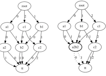
Consider the problem of generating sequences of three letters, defined on three variables (x1,x2,x3), using the alphabet {a, b, c}, that contain at most one a and at least one b, thus the combination of the problems from the previous example. Consider the MDD from Figure 1.2. This MDD is the intersection of the MDDs representing the two constraints AtMost one a and AtLeast one b from Figure 1.1. Thus all the solutions of this MDD do not contain more than one a but they all contain at least one b. This MDD represents the combination of the two constraints.
1.1. Introduction and Motivation 5 a b c b c a b c b a c b c b a b c
Figure 1.2: The intersection of the two MDDs from Figure 1.1. Thus all the solutions do not contain more than one a but do contain at least one b.
In order to efficiently manipulate MDDs, we need efficient algorithms for these three operations. Most of the existing methods fail to handle large do-mains, while many applications have large size domains (greater than 10,000 values). A good example is the MaxOrder problem [Papadopoulos 2014] (Chapter 17), it has a domain size of 11,000 in some of our instances. The existing MDD algorithms fail to solve it in a reasonable amount of time. The first goal of this thesis is to improve these algorithms. Thus we propose new algorithms for each of the operations. The main idea is to use the facts that an MDD is defined over a fixed set of variables, and that the domains can be large but sparse for the nodes. Moreover, most of the existing algorithms use complex internal data structures that, as we will show, slow down the compu-tation and restrict the addition of features. We propose to remove these data structures and design conceptually simpler and more efficient algorithms.
Creation. One good reason for using MDDs is that they can be created from many sources, for example, they can be built from Boolean formulas or dynamic programming [Hooker 2013]. Thus in this thesis we focus on im-proving some of the existing conversion, like the ones from tables or automa-ton, and we propose new creation methods for several existing compressed data structures like the global cut seed [Focacci 2001] and the tuple sequences [Régin 2011].
Reduction. MDDs are often used because of their strong compression power, which mostly comes from the reduction of the MDD. The reduction of an MDD is an operation which merges equivalent nodes. Throughout the years, several algorithms have been proposed [Andersen 1997, Brace 1991,
6 Chapter 1. Introduction is especially well suited for large set of different values.
Combination. Consider a problem containing p constraints, building an MDD for each constraint and intersecting them lead to an MDD contain-ing all the solutions of the problem. Even if such a method is not always possible, combining MDDs often drastically improves the resolution time. Combining MDDs is a well studied topic, and as for the reduction, sev-eral algorithms have already been proposed [Andersen 1997,Bergman 2014b,
Brace 1991, Bryant 1986, Bryant 1992]. In this thesis, we propose to study the existing algorithms, enlightening some of their weakness and proposing new versions strengthening them.
Advanced operations Thanks to the simple definition of our new algo-rithms for the reduction and combination, we are able to improve and extend them: 1) by designing parallel algorithms. 2) by considering relaxed MDDs. 3) by considering non deterministic MDDs.
Parallel versions of algorithms for BDDs or MDDs have been studied [Bergman 2014a,Kimura 1990,Stornetta 1996], but most of these works were limited because of the complex data structures they used for building, com-bining or reducing MDDs. Since the algorithms we propose for the reduction and combination of MDDs avoid such data structures, a new parallel algo-rithm can be design for both these algoalgo-rithms. These parallel algoalgo-rithms are designed to dispatch independent work between workers and are lock-free.
The relaxation of MDDs have been successfully applied in optimiza-tion and constraints solving [Andersen 2007,Bergman 2016b,Bergman 2011,
Cire 2013, Cire 2014b, Hadzic 2008, Hoda 2010, Hooker 2007]. The authors designed several methods for building relaxed MDDs, i.e. MDDs representing a super set of the solutions. These methods have been integrated into solvers, for example for extracting lower bounds of solution cost, and some solvers are even fully based on relaxed MDDs. In this thesis, we propose to take a look inside the algorithms. Existing works mostly focus on relaxing the creation of MDDs. Firstly, we propose to improve these creation methods. Secondly, we define the notion of relaxed reduction for MDDs, and we give an asso-ciated algorithm. Thirdly, we define the notion of relaxed combination and design two associated algorithms. Finally, we propose to analyze the available possibilities (e.g. relax creation, relax combination...) for the modeler while constructing its problem relaxation.
Non deterministic Finite Automaton (NFA) are well know in automata theory for their efficient representation that can gain an exponential factor in space against classical Deterministic Finite Automaton (DFA). This idea has been applied to MDDs several times [Bollig 1999, Finkbeiner 2001], but almost all the works have focused on restricted versions of non-determinism.
1.1. Introduction and Motivation 7 We propose in this thesis to study the simplest non-deterministic version of MDDs that allows a node to have several outgoing arcs labeled by the same value. Using this representation, we define combination algorithms that out-put both deterministic and non deterministic MDDs. Thanks to this algo-rithm, we will be able to design a new and original propagator handling the cost-MDD constraint in CP solvers.
These three features are non exclusive and can be combined. The resulting algorithms are parametric algorithms handling both deterministic and non deterministic MDDs, applying relaxation if necessary, and running in parallel. Sampling In the context of artificial intelligence, sampling is a useful tech-nique. Sampling usually consists in randomly generating sequences or val-ues, with respect to a probability distribution. Sampling under constraints is at least as hard as solving the involved CSPs, thus several works fo-cus on a restricted subsets of constraints [Jurafsky 2014, Papadopoulos 2014,
Papadopoulos 2015]. MDDs are well suited for combining constraints. We study in this thesis how to sample solutions of an MDD with respect to a probability distribution, that can be given either by a Markov chain or by a Probability Mass Function (PMF).
MDDs and solvers Constraint Programming mostly focuses on solving discrete CSPs and COPs. CP solvers, allow to define problems by their sub-problems (constraint) and the propagation mechanism combines them during the search. Embedding MDDs into solvers is one of the challenges for benefiting of their efficient compression and expressivity power. Several works have been focused on designing efficient propagator algorithms allow-ing to use MDDs in constraint programmallow-ing solvers [Cheng 2010,Cheng 2008,
Gange 2011]. Moreover, even a state of the art modeling language allows to directly define MDD constraints [Boussemart 2016]. In this thesis, we pro-pose to define a new MDD propagator for constraint solvers, which is simple, has a good complexity, and which almost always improves the resolution time compared to the existing ones. Furthermore, this MDD algorithm has been implemented in several state of the art CP solvers, such as Or-Tools and OscaR [Perron 2013, OscaR Team 2012].
MDDs can also represent optimization problems, usually this is done by adding a cost to the arcs of the MDDs, the resulting MDDs are called cost-MDDs. Several works have focused on optimization and MDDs, and in the context of constraint programming, several algorithms handle these cost-MDDs [Demassey 2006, Gange 2013]. In this thesis we propose a new algorithm for handling cost-MDD, which improves existing algorithms in all tested instances. Furthermore, we propose a new technique that allows to
8 Chapter 1. Introduction convert cost-MDD constraints into simple MDD constraints, by using the non-deterministic operations. This allows any simple MDD propagator to handle cost-MDD constraint. Note that these converted cost-MDDs can also be used into other areas than constraint programming, like satisfiability solvers.
Several problems do not contain any solution, they are called over-constrained problems. Consider for example the problem of generating a word, which has to contain at least one a, one b and two n, but whose length has to be less than 3. This problem is unfeasible. In constraint programming, over-constrained problems are often defined using soft constraints. A soft constraint is a constraint which can be violated, but with respect to a viola-tion measurement. The goal is then to find the soluviola-tion minimizing the total amount of violations. Soft constraints are well known in constraint program-ming, but soft MDD algorithms have never been investigated. Thus in this thesis we focus on designing several algorithms allowing to handle soft MDD constraints.
Modeling with MDDs The size of the MDD representing the allDifferent constraint grows exponentially. This implies that building an MDD repre-senting all the solutions of a problem is not always a good idea. Intersecting two constraints allows to extract all the solutions respecting both of the con-straints. But for intersecting two constraints using MDDs, we first need to define the two MDDs, which can already be exponential for some constraints such as the allDifferent constraint. Then, the intersection of two MDDs can lead to an MDD having as size the product of the size of two MDDs. Thus several work focus on kind of relaxed version of the intersection of constraints onto MDDs [Hoda 2010] in order to avoid these memory issues.
In this thesis we design a channeling constraint for MDDs. This constraint allows to link the values and the variables of sub-sets of arcs of an MDD with other constraints. This new method allows to define new constraints in CP solvers based on MDDs. Our best example is the Allen constraint. This con-straint aims at constraining the values of variables occurring during temporal sequences. Constraining variables using temporal sequences is often hard to define because the indexes of the variables do not necessarily correspond to their temporal positions. The propagator of this constraint uses our MDD propagators, incremental version of combinations of MDDs that we designed and the channeling constraint for MDDs. This model allows to solve instances orders of magnitude faster than other methods.
Constraint programming solvers are efficient because they have a specific algorithm for each sub-problem (constraint). But this implies a lot of code and time since the number of constraints is huge [Beldiceanu 2012]. Several works
1.2. Contributions and Outline 9 focus on reformulating constraints into others, allowing to implement and define only a sub-set of algorithms and using them to handle many constraints [Lhomme 2012]. In this thesis, we propose to reformulate existing constraints, like the dispersion and thus spread constraints [Pesant 2005, Schaus 2014,
Pesant 2015] into MDD constraints.
Thanks to the proposed methods of this thesis, several models have been designed for solving the three following industrial applications, and excellent results have been obtained. First the geomodeling of a petroleum reservoir, based on probability and knapsack constraints. Second, the Maxorder prob-lem, aiming at generating sequences avoiding plagiarism. Finally, a musi-cal synchronization problem, solved using the proposed propagators and our model, which outperforms by orders of magnitude other methods.
1.2
Contributions and Outline
1.2.1
Inside this thesis
Most of the work of this thesis consists in improving the definition of models for solving problems and in designing their associated algorithms. Next chapter is a reminder of the state of the art about decision diagrams and gives several notations used all along. The thesis is divided into five parts.
PartIfocuses on the three fundamental operations for MDDs: The
reduc-tion (Chapter 3), by giving a new algorithm that is very efficient in practice. The creation (Chapter 4), by improving several existing MDD constructors like the one from table and by proposing several new ones. The combination (Chapter 5), by proposing a new algorithm based on set operations instead of composition of functions, which is simple and efficient, and avoids com-plex data structures. Note that these improvements solve one of the problems defined in the application part of this thesis (Chapter 17).
Part II presents efficient parallel versions of the reduction and
combina-tion algorithms (Chapter 6). Lock-free algorithms having independent work loads, allowing to distribute the load over several computers are given. Then it deals with modification of our algorithms in order to handle non-deterministic MDDs (Chapter7). Next it focuses on the existing relaxation for MDD (Chap-ter 8) and proposes to take a look inside them and to design new algorithms in order to define efficient relaxations. This is done by designing operations
10 Chapter 1. Introduction like the reduction or the combination producing relaxed MDDs. Note that these three modifications are non exclusive.
This part also focuses on designing efficient sampling algorithms for MDDs (Chapter 9), by considering the two most used statistical distribution, the Markov process and the Probabiliy Mass Function (PMF). Thus this chapter defines algorithms for both of them, incremental modifications and parallel updates.
Part III focuses on the algorithms used in CP solvers for handling pure
MDD constraints. First the GAC4R algorithm is presented (Chapter 10). This new algorithm allows to efficiently handle table constraints, and is used to design MDD4R, the algorithm handling MDDs inside CP solvers that we proposed. Second, the cost version of MDDs is studied (Chapter 11), and the cost version of MDD4R is proposed, all along with another technic converting cost MDD constraints into classical MDD constraints. Third, the soft version of the MDD constraint is studied (Chapter 12), and we propose three dif-ferent methods for handling them, all with difdif-ferent efficiencies and levels of consistency. Finally, we propose a channeling constraint for MDD allowing to constrain only sub-part of the MDD (Chapter13), by constraining the allowed (or prohibited) values and variables
PartIVfocuses on defining existing or new constraints using the proposed
MDD algorithms. First the Allen constraint is defined (Chapter 14), a con-straint enforcing temporal concon-straints on variables. Then, an MDD version of the well known Spread and dispersion constraints is given (Chapter 15), all along with several others statistical constraints based on Markov processes and PMF.
Part V is about the applications we solved during this PhD thesis. The
first one is a problem of generating sequences following a Markov generation process but avoiding plagiarism from a corpus (Chapter 17). This applica-tion is mostly solved using the operaapplica-tion defined in Part I. The second one is another generation problem consisting in generating sequences of musical notes for several instruments (Chapter 18). This problem imposes temporal synchronization points as constraints. Furthermore, the generated sequences have to follow a Markov generation process. Our model uses the constraints defined in both Part III and Part IV. The last application is about the geo-modeling of a petroleum reservoir (Chapter 19), our model use several of the statistical constraints defined in Chapter 15.
1.2. Contributions and Outline 11 The work presented in this thesis mostly comes from the following pub-lications: [Perez 2017b, Perez 2016, Perez 2015a, Perez 2014, Perez 2017a,
Perez 2015b, Perez 2017c, Roy 2016]. Chapters 6, 7, 8 and a part of 13 are still under submission.
1.2.2
Other Contributions
During my PhD I had the chance and opportunity to work with many other researchers about different topics other than MDDs. This section is dedicated to them.
In the context of machine learning and optimization, I worked with M. Bar-laud and his team on the design and implementation of algorithms for numer-ical optimization, on splitting algorithms and on the design and implemen-tation of and algorithm for the projection onto the simplex and the L1 ball.
This collaboration led to the writing of both a paper in the French conference of the domain and a journal paper currently under submission.
In the context on constraint programming, I worked with several re-searchers (all the authors of [Demeulenaere 2016]), about the design of an efficient table constraint propagator. This collaboration led to a publication to the CP conference of 2016 too. Moreover, this algorithm is becoming one of the state of the art algorithm for table constraints.
In parallelism and constraints, with my supervisor J.-C. Régin. I designed and implemented a search strategy selector based on active learning algorithms (i.e Bandit, UCB) for the paper [Palmieri 2016].
Last but not least, I had worked with Anthony Palmieri, another PhD student currently at Huawei Paris, and a long time friend, about optimization, search strategies and search hybridization. This collaboration led to an article under submission.
Chapter 2
Definitions & Related Work
Contents
2.1 Definitions and Notations . . . 13 2.1.1 Constraint Programming. . . 13 2.1.2 Multi-valued Decision Diagrams . . . 14 2.2 Related Work . . . 16 2.2.1 Automaton . . . 19
2.1
Definitions and Notations
2.1.1
Constraint Programming
Constraint Programming (CP) is a problem-solving method. In CP, a prob-lem is first modeled, using variables and constraints. Usually, each variable is defined by its domain, corresponding to its set of possible values. Each con-straint defines a property that must be satisfied by a subset of the variables.
A Constraint Satisfaction Problem (CSP) is a couple P = (X, C), where X = x1, x2, ..., xN is a set of variables and C = C1, C2, ..., Cm is a set of
constraints. Each variable xiis associated with its domain D(xi), representing
all its possible values. A constraint Ci associated with a set of all allowed
tuples T (Ci) defined over a subset of variables S(Ci) ⊆ X.
A solution is a tuple of values (a1, a2, ..., ak) such that the assignment
x1 = a1, x2 = a2 ..., xN = aN satisfy all the constraints.
The resolution of a CSP generally involves a Depth First Search (DFS) algorithm using backtracking building a search tree. At each node of this tree, a propagation algorithm is run. This algorithm removes the inconsistent values with respect to the constraints. This is done by running a specific filtering algorithm associated with each constraint, called the filtering algorithm (or propagator). This filtering algorithm removes values that cannot belong to a solution of the constraint and so reduces the search space. The DFS algorithm is driven by a search strategy, usually choosing the next couple variable value to affect.
14 Chapter 2. Definitions & Related Work
Figure 2.1: An MDD representing the tuple set {(a,a),(a,b),(c,a),(c,b),(c,c)} Constraints In constraint programming, a constraint can be defined in sev-eral ways, the simplest one is to define the constraint by all its allowed tuples, thus by a table T having λ = |T | tuples. But a constraint can be defined by relation between variables, for example by enforcing that x1 < x3. Moreover,
in CP, complex constraints exist, like the allDifferent [Régin 1994], enforcing that the value taken by the variables are pairwise different. Or the atMost constraint preventing a value to appear more than a given number of times. Applications Constraint programming is often used in product line scheduling for industrial factories [Régin 1997, Bergman 2014b]. Moreover, CP is often used in crew and nurse scheduling in hospitals [Pesant 2004,
Demassey 2006, Schaus 2009b]. While this list is not exhaustive, CP is often used in industrial application of Bin-Packing, etc [Schaus 2009a,Schaus 2012,
Bent 2004]. In addition, CP is used in transportation, by managing crews, gates and flights or in configuration problems [Sabin 1996, Hadzic 2004].
Most of the applications presented in this thesis are mainly from the Artificial Intelligence area, based and the seminal works of Pachet and his team in the context of content generation for entertainment [Barbieri 2012,
Pachet 1999, Pachet 2014, Pachet 2001, Pachet 2011, Papadopoulos 2014]. Thus chapters 17 and 18 present applications that have mainly been real-ized with them. The last application presented in this thesis came from an industrial problem about the geomodeling of a petroleum reservoir.
2.1.2
Multi-valued Decision Diagrams
Multi-valued decision diagram (MDD) is a multiple-valued extension of BDDs [Bryant 1986, Akers 1978]. MDD is a rooted directed acyclic graph (DAG) often used to represent some multi-valued function f : {0...d − 1}r →
2.1. Definitions and Notations 15 The DAG representation is designed to contain r + 1 layers of nodes, such that each variable is represented at a specific layer of the r first layer of the graph, and such that the last layer represent both the true and false terminal nodes (the false terminal node is typically omitted). Each node on a given layer has at most d outgoing arcs to nodes in the next layer of the graph. Each arc is labeled by its corresponding integer.
When the MDD is used to represent a function f, there is an equivalence between f(v1, ..., vr) = trueand the existence of a path from the root node to
the true terminal node whose arcs are labeled v1, ..., vr. Figure 2.1 shows an
example of MDD defined on two variables.
Notation An MDD G = (N, E) has n = |N| nodes and m = |E| edges. A node u has a list ω+(u) of outgoing arcs and a list ω−(u) of incoming arcs.
ω+(u)[i] is the ith arc and |ω+(u)| is the number of arcs in the list . An arc
is a triplet e = (u, v, a), where u is the emanating node, v the terminating node and a the label. If the MDD is a cost-MDD, an arc is a quadruplet e = (u, v, a, c), where u is the emanating node, v the terminating node, a the label and c the cost.
16 Chapter 2. Definitions & Related Work
Figure 2.2: A simple switching circuit from [Lee 1959]
2.2
Related Work
One of the seminal work on design and analysis of circuits comes from Shannon [Shannon 1938,Shannon 1949]. The famous shannon decomposition considers that a Boolean function f(x1, x2, ...xk) can be recursively decomposed into
x1f (1, x2, ...xk) + x1f (0, x2, ...xk).
For example, consider the function f(x1, x2, x3) = x1x2x3 + x1x2x3 +
x1x2x3+ x1x2x3. Applying the Shannon decomposition on the first variable
gives :
f (x1, x2, x3) = x1f (1, x2, x3) + x1f (0, x2, x3)
f (x1, x2, x3) = x1(x2x3+ x2x3+ x2x3) + x1(x2x3)
f (x1, x2, x3) = x1(x2 + x3) + x1(x2x3)
The origin of Binary Decision Diagrams come from the Binary Decision Programs defined by Lee [Lee 1959] for representing switching circuits and in order to "compare its representation with the algebraic representation of Shannon".
In such circuit, a switch can have a value, either 0 or 1, corresponding to its current state. Figure 2.2 shows an example, coming from [Lee 1959], of such a circuit. In this circuit, x indicates that x = 1 and x indicates that x = 0.
2.2. Related Work 17 Figure 2.2 can be given as follows:
F (x, y, z) = xyz + xyz + xyz
F (x, y, z) = xF (1, y, z) + xF (0, y, z) F (x, y, z) = x(yz + yz) + x(yz)
F (x, y, z) = xyF (1, 1, z) + xyF (1, 0, z) + xyF (0, 1, z) + xyF (0, 0, z) F (x, y, z) = x(y(z) + y(z)) + x(y(z) + y(0))
F (x, y, z) = x(y(z(0) + z(1)) + y(z(1) + z(0))) + x(y(z(1) + z(0)) + y(z(0) + z(0))) F (x, y, z) = x(y(z(1)) + y(z(1))) + x(y(z(1)))
A Binary Decision Program is a set of conditional instructions, whose, using the (inverse of) today’s standard of programming, can take the form:
T → x? A : B
Meaning that if the value of x is 0 then go to instruction A, otherwise go to instruction B. Note that each instruction is associated with a variable.
Thus for the switching circuit of Figure2.2, we obtain the following binary decision program: 1 → x? 2 : 4 2 → y? F : 3 3 → z? F : T 4 → y? 3 : 5 5 → z? T : F
Such a program describes all the possible paths of the circuits. As we can see, compared to the Shannon decomposition, the function z is shared.
Several years later, Akers [Akers 1978] introduce the Binary Decision Dia-gram, as a graphical structure. These BDDs were used to represent switching functions extracted from the switching networks. As said before, the Binary Decision Diagrams can have two outgoing arcs, labeled by either 0 or 1, di-rected to the next layers and two terminal nodes 0 and 1. The arcs labeled by 0 are usually dashed in graphical representation.
Consider for example the BDD from Figure2.3that represented the Binary Decision Program defined for the switching circuit of Figure 2.2. This BDD shows the sharing of the node 3.
18 Chapter 2. Definitions & Related Work 1 2 4 F 3 5 T
Figure 2.3: A BDD representing the switching circuit from Figure 2.2
In 1986, Bryant [Bryant 1986] published a groundbreaking work about BDDs. Bryant proposed to impose a total ordering on the variables of the BDD, introducing the Ordered Binary Decision Diagrams. Thanks to this, Bryant proposed many algorithm allowing to efficiently combine BDDs. Fur-thermore, using this total ordering, Bryant was able to reduce the OBDD into a canonical form giving the Reduced Ordered Binary Decision Diagrams (ROBDDs) which are widely used, and most of the time, BDD stands for Bryant’s ROBDDs. In its works, Bryant distinguished the three important operations for BDDs which are the creation, the reduction and the combina-tion.
The creation of BDDs and MDDs have been studied many times, as shown for building BDDs from Boolean formulae [Bryant 1986,Andersen 1997]. But since several years, BDDs and MDDs are built from many other sources, consider for example the work of Cheng and Yap [Cheng 2008, Cheng 2010,
Cheng 2005] which builds MDDs from set of tuples or sub-problems. More about their work is given in chapter 4.
Moreover, several researchers aimed at building MDDs from dynamic programming [Hooker 2013, Bergman 2016b], by extracting a set of states and a transition function. Furthermore, they have made a seminal work on compiling constraint satisfaction problems (CSPs) and constraint op-timization problems onto MDDs and in the analysis of their complexity [Hadzic 2008, Andersen 2007]. For example, in using an MDD as a domain store instead of classical set of values, which has helped solve several hard combinatorial problems.
2.2. Related Work 19 Andersen et al. [Andersen 2007] proposed to limit the size of the MDD by limiting the number of nodes. Such MDDs are called the relaxed MDDs, since they are discrete relaxations of the constraints they represent. These relaxed MDDs usually represents super set of the solution, instead of the exact set of solutions. They can be built while compiling the CSPs, like in [Hadzic 2008], or by separation of the constraints [Ciré 2014a]. Another relaxation named the restricted Decision Diagrams have been introduced [Ciré 2014a] to represent a subset of the solutions, instead of a super set. One of the advantages of such relaxation is that the cost of a solution found in this restricted DD is a lower-bound of the best solution.
In the context of constraint programming, many works can be found. The first MDD propagator has been given by Cheng and Yap in [Cheng 2008,
Cheng 2010], then several MDD propagators has been designed [Gange 2011,
Perez 2014], all these works allow CP solvers to directly handle an MDD stor-ing all the satisfystor-ing or prohibited tuples. Nowadays, almost all the CP solvers have an MDD constraint and MDDs are even part of the standard XCSP for-mat [Boussemart 2016], and MDD where also available since 2000 in SICStus [Carlsson] and used to implement the transition constraints associated to the reformulation of an automaton, but without minimization.
In addition to these propagators, several works focus on constraining the MDD himself [Hoda 2010, Bergman 2014b], by, for example, enforcing that the cost of all the paths is in a given interval. Andersen et al. [Andersen 2007] have introduced the notion of MDD consistency, which enforces that each arc belongs to at least one solution.
Several distinct subjects are studied in this thesis, thus many chapters start with a related work section focusing on the exact subject of the chapter.
2.2.1
Automaton
Automaton have been often used in Constraint Programming. A deter-ministic finite automaton [Hopcroft 2006] can be represented by a 5-tuple (Q, Σ, δ, q0, F ) with :
• A finite set of states Q
• A finite set of symbols Σ (the alphabet)
• A transition function δ between states. Q x Σ → Q • An initial state q0
20 Chapter 2. Definitions & Related Work • A set of accepting states F .
An automaton accepts a word (sequence of symbols s1,s2...sn∈ Σ) if there
exists a set of transition {(q0, s1, q1), (q1, s2, q2), ..., (qn−1, sn, qn)} and that qn
is an accepting state. The set of words accepted by an automaton is called the language of the automaton. The minimal automaton for a given language is the automaton recognizing the language and having the smallest number of state.
Example:
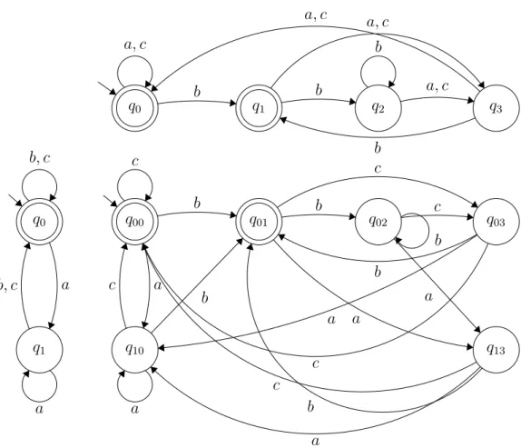
Let Σ = {a, b, c}. Consider the following automaton preventing ac-cepted words to finish by an a:
q0 q1
a b, c
b, c
a
This automaton is not really complicated, and is readable.
It can be challenging to define automatons. This is often due to their ability to accept words of arbitrary sizes.
Example:
Consider the following automaton preventing accepted words to have a b in the before last position:
q0 q1 q2 q3 b a, c a, c b b a, c b a, c
This automaton is not trivial anymore.
Combining automaton accepting words of arbitrary sizes is often harder than solving the problems with MDDs having fixed size.
2.2. Related Work 21
Example:
Consider the automatons of the two previous examples. The product automaton of these automatons is given in Figure 2.4. This automaton represents the words that cannot finish by an a and not having a b in the before last position. It is almost unreadable for human.
These two simple unary constraints can be easily enforced with MDDs. Figure 2.5 shows the resulting MDD while applying the constraints over 3 variables. This MDD is simple and readable. This example shows that MDDs are well suited for fixed size words generation.
Even avoiding the fact that defining automaton is challenging, some simple unary constraints can lead to automatons having an exponential size, while the MDD has a linear size.
Example:
Consider the generalization of the previous examples, the language (a|b|c)∗a(a|b|c)n. The DFA representing this language has 2n+1 nodes. The case with n = 0 and n = 1 are the two previous examples. A Non-deterministic Finite Automaton (NFA) can represent this language using n + 1 nodes. An MDD defined over k variables represents this language using k nodes, see Figure2.5.
This example shows that an MDD can have comparable compression power to NFA. Furthermore, NFA can have an exponential compression power against DFA. The proposed example shows an MDD having an exponential factor of compression against DFA.
22 Chapter 2. Definitions & Related Work q0 q1 q2 q3 q0 q1 q00 q10 q01 q02 q03 q13 b a, c a, c b b a, c b a, c a b, c a b, c c a c a b b a b c b a c a c b b a c
Figure 2.4: Intersection of two automatons representing unary constraints.
r
a bc
a c
tt
b c
Figure 2.5: MDD representing solutions of two unary constraints over three variables.
Part I
Chapter 3
Reduction
Contents
3.1 Introduction . . . 25 3.2 Related Work . . . 27 3.3 pReduce, a linear reduction operator. . . 30 3.3.1 ipReduce, Incremental reduction . . . 33 3.4 Experiments . . . 37
3.1
Introduction
One of the main advantages of MDDs is their compression. MDDs are able to gain an exponential factor in representation space, but to do so MDDs have to be reduced. Reduction is an operation which consists of transforming an MDD into its smallest canonical form, for a given variable ordering [Bryant 1986]. This is one of the most important operations for MDDs.
Reduction operation merges equivalent nodes. Two nodes are equivalent if they have the same outgoing labeled paths.
Definition 1 Two nodes u and v are equivalent, denoted by u ≡ v, if: |ω+(u)| = |ω+(v)| ∧ ∀(u, w, a) ∈ ω+(u), ∃(v, w, a) ∈ ω+(v) (3.1)
Nodes that have the same outgoing arcs can be easily merged. This is done by redirecting all incoming arcs of all the nodes to only one, and then removing the ones that do not have any more incoming arcs.
By using this definition for merging nodes, in a bottom up fashion, we can find all the equivalent nodes.
Proof If two nodes at layer i are equivalent, after reduction of the layer i + 1, they have the same outgoing arcs. This property is true for the last layer, and recursively true for the other layers.
26 Chapter 3. Reduction
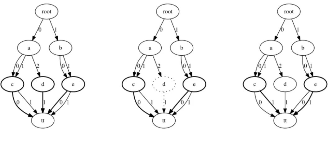
Example:
Consider the MDDs from Figure3.1. This example shows the merging of the two equivalent nodes, e and c.
In the left MDD, both the nodes c and e have arcs labeled by 0 and 1 and directed to the node tt, these two nodes are equivalent. This implies that we can merge them. The right MDD shows the MDD after the merging of nodes, the resulting node being the node ce. As we can see in this MDD, even if both a and b nodes have arcs labeled by 0 and 1 directed to the node ce, these two nodes are not equivalent since the node a has an arc labeled by 2 and directed to the node d.
When no more nodes can be merged, an MDD is said to be reduced. Note that the order in which nodes are merged has no impact since a reduced MDD, for a given variable ordering, is on a canonical form [Bryant 1986].
We can denote a Reduced Ordered MDD by the acronym ROMDD. In this thesis, for the sake of clarity, the acronym MDD is going to be used instead of ROMDD.
Figure 3.1: Example of reduction.
The problem Define a reduction algorithm finding all the equivalent nodes efficiently.
3.2. Related Work 27 Plan This chapter is split in three parts. The first one describes the state of the art methods for reducing MDDs or BDDs. The second one introduces pReduce, a reduction algorithm, linear on the number of arc, and one of the contributions of this thesis. The third one proposes ipReduce, an incremental reduction version of pReduce.
3.2
Related Work
Several algorithms for reducing MDDs and BDDs exist [Bryant 1986,
Cheng 2010, Andersen 1997, Brace 1991]. This section describes some of them.
One of the classical representations for MDDs is to represent each node by an array of outgoing arcs (cf Appendix A.1). The size of this array is fixed and is the size of the domain (d). Using this representation, the existence of an arc labeled by i is given by the value of the ith cell of this array. If the value
is ff then the arc does not exist, otherwise the cell contains the terminating node of the arc.
The access of the outgoing arc of node u labeled by i is denoted by u[i]. Using this representation, two nodes u and v are equivalent iff:
∀i ∈ [1, d], u[i] = v[i] (3.2)
Example:
Considering the MDD from Figure 3.1, the nodes c, d and e have the following arrays of outgoing arcs:
Node 0 1 2
c tt tt ff
e tt tt ff
d ff tt ff
The nodes c and e have the same line (array of nodes), that is why they are equivalent.
Main idea The main idea behind a lot of reduction algorithms is to perform a search on the MDD and to merge equivalent nodes by memorizing all the already visited nodes in a data structures.
These algorithms usually process a DFS inside the MDD. During the post-visit, they use a dictionary-like data structure to search for a similar node of the current node. This kind of method has a complexity of O(n ∗ D) with
28 Chapter 3. Reduction Algorithm 1Reduction of an MDD using the classical DFS and a Dictionary. reduce(M ) define D root(M) ← reduceDFS(root(M),D) reduceDFS(u, D) if ∃v ∈ D, u ≡ v then return v for each i ∈ [0, d] do u[i] ← reduceDFS(u[i],D) if ∃v ∈ D, u ≡ v then return v Add(D,u) return u
D the complexity of using a dictionary for finding equivalent nodes. The Algorithm 1is a possible implementation of such algorithm.
Dictionary There are two ways for implementing such a dictionary that deserves some attention: by a radix tree or by a hash table.
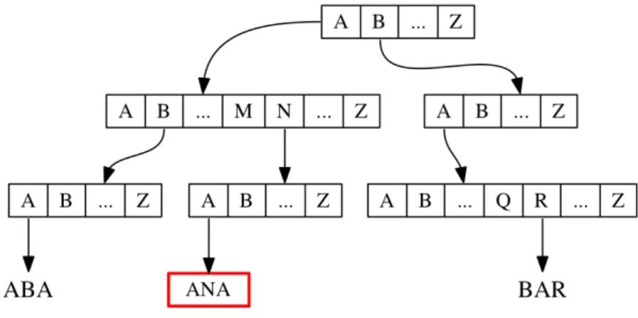
A radix tree is a tree used to store words such that each node contains an array of outgoing edges of size |Σ|, where Σ is the alphabet of the words. To check if a word belongs to the radix tree, we have to check if a path using the letters of the word exists. An example of radix tree is given in Figure 3.2.
The use of a radix tree with words of size d having n different values gives a tree having d layers such that each node is an array of size n (n is the number of nodes of the MDD). Using this radix tree, looking for an equivalent node can be done in O(d), and the insertion of a node may lead to the creation of d nodes of size n. This prevents us from using such a data structure.
That’s why most algorithms use hash tables. In this case we cannot ensure reaching a O(d) time complexity but we can expect the search in the table to be close to O(1) once the hash code of the key has been computed, which is in O(d). Such a result can be obtained by using a table whose size is greater than n when n elements are involved. The drawback of this approach in practice is that it may be time consuming to compute an efficient hash code and it needs a large table when we do not know n in advance.
Advantages This reduction method can be useful while performing opera-tions like the Apply operator (see Chapter 5) on MDDs because it can reduce the MDD while performing the operation.
3.2. Related Work 29
Figure 3.2: A radix tree containing the words ANA, ABA and BAR. The word ANA is obtained by following the path A->N->A in the tree.
Example:
Consider the MDDs from Figure 3.1. This example shows the appli-cation of the classical reduction method to the MDD on the left.
First, the algorithm processes a DFS and the post visit of the DFS stores the nodes in a Hash map. Starting from the root node. Using the values in the lexicographic order, this leads us to node c. Node c has 0tt1tt as signature, and thus is put in the associate cell of the hash map. The algorithm then goes at node d and put this node in the cell associated to signature 1tt. Then the algorithm goes to node a and put it in cell 0c1c2d. The next studied node is e with signature 0tt1tt. Node c already has this signature, thus this two nodes are merged. This is done by returning c instead of e. The next processed node is b with signature 0c1c, no node has the same signature, thus b is put in the Hash map. The result is the MDD on the right.
More Bryant [Bryant 1986] proposed an algorithm for BDDs that associates a unique key to each node based on their outgoing arcs. The nodes are then sorted and the algorithm checks for each two-consecutive nodes if they are equivalent (i.e. if their unique key is the same). With d = 2, a unique key based on the outgoing arcs can easily be generated, but generating a unique key to any d > 2 is costly. The next section shows how to do it incrementally without necessarily check all the arcs.
30 Chapter 3. Reduction
3.3
pReduce, a linear reduction operator
This section presents pReduce, named from "pack reduce", a reduction algo-rithm whose time complexity per node is bounded by its number of outgoing arcs and not by the number of possible values (d). In addition, the time and memory complexities are both linear on the size of the MDD O(n + m).
This algorithm is close to the algorithm proposed for acyclic deterministic automaton [Revuz 1992] which performs a kind of lexicographic sort of nodes using bucket sort. But here, each bucket is going to be split by looking at the next arc, and thus the complexity is bound by the number of arcs instead of being quadratic.
This algorithm can be seen as an incremental version of the algorithm first proposed for BDDs [Bryant 1986]. Note that the direct application would have used a raddix sort, using as base the number of possible values, but the complexity would have been quadratic O(d ∗ n).
Representation The pReduce algorithm uses the ω+ list implementation of an MDD (Appendix A.2). The particularity of this list of outgoing arcs is that they are ordered by their label. Thanks to several creation and operation algorithms presented in this thesis, we can assume that this property is always ensured.
Example:
Considering the MDD from Figure 3.1, the nodes c, d and e have the following lists of outgoing arcs:
Node ω+
c {(0,tt),(1,tt)}
e {(0,tt),(1,tt)}
d {(1,tt)}
Main idea Instead of checking for each node if there exists an equivalent node in the MDD, pReduce tries to build clusters of equivalent nodes.
From equation (3.1), two nodes are equivalent if they have the same num-ber of outgoing arc, and for each pair (label, destination) from the ω+ of the
first one, there is a pair (label, destination) in the second one.
Let the equal = and not equal 6= operators between two arcs be operators comparing both the label and the destination. Since the ω+ lists of arcs
are sorted by the label, we can apply the function of equivalence given in Algorithm 2.
3.3. pReduce, a linear reduction operator 31 Algorithm 2Equivalence of two nodes.
equivalent(u, v)
if |ω+(u)| 6= |ω+(v)| then
return False
for each i ∈ 1..|ω+(u)| do
if ω+(u)[i] 6= ω+(v)[i] then
return False return True
This equivalent function compares the outgoing arcs of two nodes while they are the same and stop at the first difference.
The pReduce algorithm performs this equivalence function incrementally over all the nodes at the same time. pReduce puts all the nodes of a layer into a set (i.e. a pack). Then it splits this set into several sets by comparing their first outgoing arc. Then for each of these new sets, it splits the nodes by comparing their second outgoing arc. The same process is applied iteratively over all the arcs until obtaining a node alone or having checked all the arcs of the nodes. When two or more nodes have all their outgoing arcs checked and they are still in the same pack, they are equivalent.
Pack A pack is a data structure. A pack p contains a set S of nodes and a position t. A pack ensures that all the nodes in S have the same prefix of t arcs in their ordered ω+ list. Formally we have:
∀u, v ∈ S, ∀(u, w, a) ∈ ω+(u)[1, t], ∃(v, w, a) ∈ ω+(v)[1, t] (3.3)
As defined in section2.1, ω+(v)[1, t]denotes the sub-list of the t first elements
of ω+(v). A pack contains all the nodes having the same first t arcs (prefix).
We denote by |p| the number of nodes inside the pack p.
Splitting a pack During the processing of a pack, pReduce splits the pack into several packs according to their t + 1th arc. A pack is created for each
pair of values (v, a) in the t + 1th arc (x, v, a) of the nodes.
pReduce Algorithm 3 is a possible implementation of the pReduce algo-rithm. It uses VA and NA two arrays of sets in order to perform the split
operation of a pack p in O(|p|). Array VA is indexed by the values and array
NA is indexed by the nodes. Note that these two arrays contain only empty
32 Chapter 3. Reduction Nlist two lists of elements that are used to save the entries that are not empty
in the arrays. At the end of the algorithm the lists are empty.
Algorithm 3 has two phases. First, it splits the current pack p into the array of sets VA according to the value labeling the arc at position pos(t) + 1.
The second phase considers each set computed in the first phase and splits its elements into the array of sets NA according to the terminating node of the
arcs. The algorithm also modifies the computed sets in order to detect nodes that can be merged and to define packs and put them into the queue Q. The time complexity of this algorithm depends only on the number of neighbors of a node, because thanks to the lists we never reach an empty cell. In addition each arc is traversed only twice: one for the value and one for the node. The space complexity is in O(n + d). The operation ω+(x)[i + 1]can be performed
by keeping the last checked arc for each node.
The reduction of the whole MDD is made by applying a BFS from the bottom to the top and by calling Function reduceLayer for each layer with L the list of nodes to merge as a parameter.
root a 0 b 1 c 0 1 d 2 e 0 1 tt 0 1 1 0 1 root a 0 b 1 c 0 1 d 2 e 0 1 tt 0 1 1 0 1 root a 0 b 1 c 0 1 d 2 e 0 1 tt 0 1 1 0 1
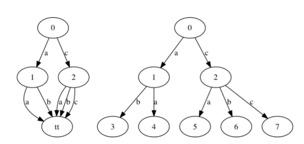
Figure 3.3: Application of the pReduce algorithm on the last layer. Example:
Consider the MDDs from Figure 3.3. This example shows the appli-cation of the pReduce algorithm to the MDD from Figure3.1.
First, all the nodes of the layer of the last variable (c,d,e) are put in a pack. Then their first arc is studied. This arc is (0,tt) for c and e and is (1,tt) for d. This is shown on the MDD on the left, remember that the arc are sorted by their label. Two packs are thus created, one containing c and e and one containing only d. The packs that contain only one element
3.3. pReduce, a linear reduction operator 33 are removed, thus the pack containing d is removed, MDD on the middle. The algorithm now processes the second arc of the pack (c,e), MDD on the rigth. This two nodes are on the same pack while no more nades has to be processed, they are equivalent.
The algorithm now processes the layer of nodes a and b, they are on the same pack for their two first arcs (0,c) and (1,c), but they are splitted since b does not have any arc to process and a is alone in its pack thus not processed.
Improvement While the complexity is already linear, we can try to improve the efficiency of this reduction algorithm by first splitting the pack of the nodes of a layer by considering the size of the ω+ list of arcs.
Complexity Since pReduce only considers the common prefix of the outgo-ing arcs list, the complexity can be defined as the sum of the common prefix of the nodes. The worst-case complexity is bounded by O(n + m + d). More This notion of pack is important, using it, we are going to modify the pReduce algorithm in order to deal with incremental modification of MDDs (next section) and parallel version of the algorithms (chapter 6).
3.3.1
ipReduce, Incremental reduction
Some algorithms presented in this thesis in chapter 5modify MDDs that was already reduced. After these modifications we want to reduce the obtained MDDs. A simple method is to apply the existing reduction algorithms. But classical reduction operations consider the whole MDD, even when small mod-ifications occur.
ipReduce is an incremental adaptation of the pReduce algorithm, allowing to save time while reducing previously reduced MDDs after their modifica-tions.
Main idea After the modification of an MDD, only modified nodes, newly created nodes or nodes having arcs directed to such nodes can lead to a merge. The idea is to consider only the packs that contain such nodes.
In order to be able to know whose nodes have been modified since the last reduction, we need to store this information inside the nodes. Let m be the field of nodes that contains a stamp whose value is the stamp of the last modification.
34 Chapter 3. Reduction The algorithm 4 is a possible implementation of this algorithm. As you can see, the first line of the iReducePack function check if the current pack contains or not a node whose m value is equal to the last modification stamp mg. Note that this can be maintained by keeping in each pack the max value
of the m values of the nodes while building it.
While the worst-case complexity of this algorithm remains the same as the non-incremental version, the advantage in practice is important. Also, this incremental version of the reduction can become the only one in an imple-mentation of an MDD package since it considers all the nodes at the creation of an MDD.