FORESTOGRAM: BICLUSTERING VISUALIZATION FRAMEWORK WITH APPLICATIONS IN PUBLIC TRANSPORT AND BIOINFORMATICS
MOHAMMAD SAJJAD GHAEMI
DÉPARTEMENT DE MATHÉMATIQUES ET DE GÉNIE INDUSTRIEL ÉCOLE POLYTECHNIQUE DE MONTRÉAL
THÈSE PRÉSENTÉE EN VUE DE L’OBTENTION DU DIPLÔME DE PHILOSOPHIÆ DOCTOR
(MATHÉMATIQUES DE L’INGÉNIEUR) DÉCEMBRE 2017
c
ÉCOLE POLYTECHNIQUE DE MONTRÉAL
Cette thèse intitulée :
FORESTOGRAM: BICLUSTERING VISUALIZATION FRAMEWORK WITH APPLICATIONS IN PUBLIC TRANSPORT AND BIOINFORMATICS
présentée par : GHAEMI Mohammad Sajjad
en vue de l’obtention du diplôme de : Philosophiæ Doctor a été dûment acceptée par le jury d’examen constitué de :
M. ADJENGUE Luc-Désiré, Ph. D., président
M. AGARD Bruno, Doctorat, membre et directeur de recherche
M. PARTOVI NIA Vahid, Doctorat, membre et codirecteur de recherche Mme MORENCY Catherine, Ph. D., membre
RÉSUMÉ
Dans de nombreux problèmes d’analyse de données, les données sont exprimées dans une matrice avec les sujets en ligne et les attributs en colonne. Les méthodes de segmentations traditionnelles visent à regrouper les sujets (lignes), selon des critères de similitude entre ces sujets. Le but est de constituer des groupes de sujets (lignes) qui partagent un certain degré de ressemblance. Les groupes obtenus permettent de garantir que les sujets partagent des similitudes dans leurs attributs (colonnes), il n’y a cependant aucune garantie sur ce qui se passe au niveau des attributs (les colonnes). Dans certaines applications, un regroupement simultané des lignes et des colonnes appelé biclustering de la matrice de données peut être souhaité. Pour cela, nous concevons et développons un nouveau cadre appelé Forestogram, qui permet le calcul de ce regroupement simultané des lignes et des colonnes (biclusters) dans un mode hiérarchique. Le regroupement simultané des lignes et des colonnes de manière hiérarchique peut aider les praticiens à mieux comprendre comment les groupes évoluent avec des propriétés théoriques intéressantes. Forestogram, le nouvel outil de calcul et de visualisation proposé, pourrait être considéré comme une extension 3D du dendrogramme, avec une fusion orthogonale étendue. Chaque bicluster est constitué d’un groupe de lignes (ou de sujets) qui déplie un schéma fortement corrélé avec le groupe de colonnes (ou attributs) correspondantes. Cependant, au lieu d’effectuer un clustering bidirectionnel indépendamment de chaque côté, nous proposons un algorithme de biclustering hiérarchique qui prend les lignes et les colonnes en même temps pour déterminer les biclusters. De plus, nous développons un critère d’information basé sur un modèle qui fournit un nombre estimé de biclusters à travers un ensemble de configurations hiérarchiques au sein du forestogramme sous des hypothèses légères. Nous étudions le cadre suggéré dans deux perspectives appliquées différentes, l’une dans le domaine du transport en commun, l’autre dans le domaine de la bioinformatique.
En premier lieu, nous étudions le comportement des usagers dans le transport en commun à partir de deux informations distinctes, les données temporelles et les coordonnées spatiales recueillies à partir des données de transaction de la carte à puce des usagers. Dans de nom-breuses villes, les sociétés de transport en commun du monde entier utilisent un système de carte à puce pour gérer la perception des tarifs. L’analyse de cette information fournit un aperçu complet de l’influence de l’utilisateur dans le réseau de transport en commun interac-tif. À cet égard, l’analyse des données temporelles, décrivant l’heure d’entrée dans le réseau de transport en commun est considérée comme la composante la plus importante des don-nées recueillies à partir des cartes à puce. Les techniques classiques de segmentation, basées sur la distance, ne sont pas appropriées pour analyser les données temporelles. Une nouvelle
projection intuitive est suggérée pour conserver le modèle de données horodatées. Ceci est introduit dans la méthode suggérée pour découvrir le modèle temporel comportemental des utilisateurs. Cette projection conserve la distance temporelle entre toute paire arbitraire de données horodatées avec une visualisation significative. Par conséquent, cette information est introduite dans un algorithme de classification hiérarchique en tant que méthode de segmen-tation de données pour découvrir le modèle des utilisateurs. Ensuite, l’heure d’utilisation est prise en compte comme une variable latente pour rendre la métrique euclidienne appropriée dans l’extraction du motif spatial à travers notre forestogramme.
Comme deuxième application, le forestogramme est testé sur un ensemble de données multiomiques combinées à partir de différentes mesures biologiques pour étudier comment l’état de santé des patientes et les modalités biologiques correspondantes évoluent hiérarchi-quement au cours du terme de la grossesse, dans chaque bicluster. Le maintien de la grossesse repose sur un équilibre finement équilibré entre la tolérance à l’allogreffe fœtale et la protec-tion mécanismes contre les agents pathogènes envahissants. Malgré l’impact bien établi du développement pendant les premiers mois de la grossesse sur les résultats à long terme, les in-teractions entre les divers mécanismes biologiques qui régissent la progression de la grossesse n’ont pas été étudiées en détail. Démontrer la chronologie de ces adaptations à la grossesse à terme fournit le cadre pour de futures études examinant les déviations impliquées dans les pathologies liées à la grossesse, y compris la naissance prématurée et la prééclampsie. Nous effectuons une analyse multi-physique de 51 échantillons de 17 femmes enceintes, livrant à terme. Les ensembles de données comprennent des mesures de l’immunome, du transcrip-tome, du microbiome, du protéome et du métabolome d’échantillons obtenus simultanément chez les mêmes patients. La modélisation prédictive multivariée utilisant l’algorithme Elas-tic Net est utilisée pour mesurer la capacité de chaque ensemble de données à prédire l’âge gestationnel. En utilisant la généralisation empilée, ces ensembles de données sont combinés en un seul modèle. Ce modèle augmente non seulement significativement le pouvoir prédictif en combinant tous les ensembles de données, mais révèle également de nouvelles interactions entre différentes modalités biologiques. En outre, notre forestogramme suggéré est une autre ligne directrice avec l’âge gestationnel au moment de l’échantillonnage qui fournit un mo-dèle non supervisé pour montrer combien d’informations supervisées sont nécessaires pour chaque trimestre pour caractériser les changements induits par la grossesse dans Microbiome, Transcriptome, Génome, Exposome et Immunome réponses efficacement.
ABSTRACT
In many statistical modeling problems data are expressed in a matrix with subjects in row and attributes in column. In this regard, simultaneous grouping of rows and columns known as biclustering of the data matrix is desired. We design and develop a new framework called Forestogram, with the aim of fast computational and hierarchical illustration of biclusters. Often in practical data analysis, we deal with a two-dimensional object known as the data matrix, where observations are expressed as samples (or subjects) in rows, and attributes (or features) in columns. Thus, simultaneous grouping of rows and columns in a hierarchical manner helps practitioners better understanding how clusters evolve. Forestogram, a novel computational and visualization tool, could be thought of as a 3D expansion of dendrogram, with extended orthogonal merge. Each bicluster consists of group of rows (or samples) that unfolds a highly-correlated schema with their corresponding group of columns (or attributes). However, instead of performing two-way clustering independently on each side, we propose a hierarchical biclustering algorithm which takes rows and columns at the same time to determine the biclusters. Furthermore, we develop a model-based information criterion which provides an estimated number of biclusters through a set of hierarchical configurations within the forestogram under mild assumptions. We study the suggested framework in two different applied perspectives, one in public transit domain, another one in bioinformatics field.
First, we investigate the users’ behavior in public transit based on two distinct infor-mation, temporal data and spatial coordinates gathered from smart card. In many cities, worldwide public transit companies use smart card system to manage fare collection. Analy-sis of this information provides a comprehensive insight of user’s influence in the interactive public transit network. In this regard, analysis of temporal data, describing the time of enter-ing to the public transit network is considered as the most substantial component of the data gathered from the smart cards. Classical distance-based techniques are not always suitable to analyze this time series data. A novel projection with intuitive visual map from higher dimension into a three-dimensional clock-like space is suggested to reveal the underlying tem-poral pattern of public transit users. This projection retains the temtem-poral distance between any arbitrary pair of time-stamped data with meaningful visualization. Consequently, this information is fed into a hierarchical clustering algorithm as a method of data segmentation to discover the pattern of users. Then, the time of the usage is taken as a latent variable into account to make the Euclidean metric appropriate for extracting the spatial pattern through our forestogram.
dif-ferent biological measurements to study how patients and corresponding biological modalities evolve hierarchically in each bicluster over the term of pregnancy. The maintenance of preg-nancy relies on a finely-tuned balance between tolerance to the fetal allograft and protective mechanisms against invading pathogens. Despite the well-established impact of development during the early months of pregnancy on long-term outcomes, the interactions between vari-ous biological mechanisms that govern the progression of pregnancy have not been studied in details. Demonstrating the chronology of these adaptations to term pregnancy provides the framework for future studies examining deviations implicated in pregnancy-related patholo-gies including preterm birth and preeclampsia. We perform a multiomics analysis of 51 samples from 17 pregnant women, delivering at term. The datasets include measurements from the immunome, transcriptome, microbiome, proteome, and metabolome of samples ob-tained simultaneously from the same patients. Multivariate predictive modeling using the Elastic Net algorithm is used to measure the ability of each dataset to predict gestational age. Using stacked generalization, these datasets are combined into a single model. This model not only significantly increases the predictive power by combining all datasets, but also re-veals novel interactions between different biological modalities. Furthermore, our suggested forestogram is another guideline along with the gestational age at time of sampling that provides an unsupervised model to show how much supervised information is necessary for each trimester to characterize the pregnancy-induced changes in Microbiome, Transcriptome, Genome, Exposome, and Immunome responses effectively.
TABLE OF CONTENTS
RÉSUMÉ . . . iii
ABSTRACT . . . v
TABLE OF CONTENTS . . . vii
LIST OF TABLES . . . x
LIST OF FIGURES . . . xi
LIST OF NOTATIONS AND ACRONYMS . . . xvi
CHAPTER 1 INTRODUCTION . . . 1
CHAPTER 2 LITERATURE REVIEW . . . 8
2.1 Hierarchical Clustering . . . 8 2.1.1 Single Linkage . . . 10 2.1.2 Complete Linkage . . . 10 2.1.3 Average Linkage . . . 10 2.1.4 Ward Linkage . . . 11 2.1.5 Centroid Linkage . . . 11 2.1.6 Median Linkage . . . 11
2.1.7 Properties of hierarchical algorithms . . . 13
2.1.8 Model-based cluster estimation . . . 14
2.1.9 Biclustering . . . 15
2.2 Application . . . 16
2.2.1 Public Transport . . . 17
2.2.2 Bioinformatics . . . 19
CHAPTER 3 RESEARCH APPROACH AND STRATEGY . . . 20
CHAPTER 4 ARTICLE 1: FORESTOGRAM: A VISUALIZATION FRAMEWORK FOR HIERARCHICAL BICLUSTERING . . . 25
4.1 Abstract . . . 25
4.3 Hierarchical Biclustering . . . 27 4.3.1 Bilinkage . . . 27 4.3.2 Forestogram . . . 27 4.3.3 Number of Biclusters . . . 28 4.3.4 Separable Biclusters . . . 32 4.4 Computational Complexity . . . 35 4.4.1 Lance-Williams Speed-up . . . 35 4.4.2 Time Complexity . . . 35 4.4.3 Space Complexity . . . 36
4.4.4 Parallel computing for dissimilarity measure . . . 37
4.4.5 R-package . . . 39
4.5 Simulation . . . 41
4.6 Application . . . 43
CHAPTER 5 ARTICLE 2: A VISUAL SEGMENTATION METHOD FOR TEMPO-RAL SMART CARD DATA . . . 45
5.1 Abstract . . . 45
5.2 Inrtoduction . . . 45
5.3 State-of-the-art . . . 46
5.3.1 Recent research papers on the analysis of smart card data . . . 46
5.3.2 Extraction of users’ temporal patterns in transportation . . . 49
5.3.3 Synthesis and justification of the needs . . . 51
5.4 Proposed methodology . . . 52
5.5 Projection properties . . . 53
5.6 Experimental results . . . 58
5.6.1 Demonstration of Semi-Circle Projection (SCP) . . . 58
5.6.2 Experimenting the SCP method on Gatineau dataset . . . 61
5.7 Conclusion and Discussion . . . 65
5.8 Challenges in Spatial Data Analysis Targeting Public Transit . . . 70
5.9 Spatial-temporal data analysis with forestogram . . . 77
CHAPTER 6 MULTIOMICS ANALYSIS OF HOST RESPONSE TO PREGNANCY 84 6.1 Abstract . . . 84
6.2 Introduction . . . 84
6.3 Results . . . 87
6.3.1 Overview . . . 87
6.3.3 Stacked Generalization . . . 89 6.4 Methods . . . 94 6.4.1 Elastic net . . . 94 6.4.2 Cross-validation . . . 96 6.4.3 Stack generalization . . . 96 6.4.4 Correlation network . . . 98 6.5 Unsupervised Analysis . . . 102 6.6 Discussion . . . 109
CHAPTER 7 GENERAL DISCUSSION . . . 112
7.1 Forestogram . . . 112
7.2 Public transport . . . 113
7.3 Bioinformatics . . . 114
7.4 Limitations of forestogram and hierarchical algorithms . . . 115
7.5 Improvement . . . 115
CHAPTER 8 CONCLUSION . . . 117
LIST OF TABLES
Table 4.1 A list of common linkages for hierarchical clustering, defined using the Euclidean distance, where ¯y denotes the mean, and ˜y denotes the median. 28 Table 4.2 Lance-Williams coefficient merge updates for different linkages, if the
Euclidean distance defines the linkage. . . 36 Table 4.3 The performance of different biclustering techniques using the average
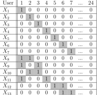
adjusted Rand index ×100. The larger the adjusted Rand index is, the better the performance will be. . . 42 Table 5.1 Synthetic example of temporal data associated to 13 users and the
cor-responding usage during 7 hours, e.g. user 1 entered the public transit in the very early hour of day where the related index is 1. . . 59 Table 5.2 Synthetic example of spatial-temporal data associated with 8 users and
the corresponding usages during 5 hours. Spatial location is denoted by (latitude, longitude) pair. . . 79
LIST OF FIGURES
Figure 2.1 A univariate example of 5 data points. . . 8 Figure 2.2 Step by step demonstration of agglomerative hierarchical clustering. . 9 Figure 2.3 Dendrograms corresponding to the four different linkages in
hierarchi-cal clustering applied to random data. As it is shown in Figure 2.3(c) monotonicity property is not satisfied for all linkages. . . 12 Figure 2.4 A typical public transit network. . . 17 Figure 3.1 Thesis contribution. . . 24 Figure 4.1 Forestogram building steps on a hypothetical 3 × 3 matrix. Left to
right: the data matrix, merging a pair of columns, merging a pair of rows, and the completed forestogram. . . 29 Figure 4.2 A hypothetical 9 × 9 matrix clustered into three row blocks and 3
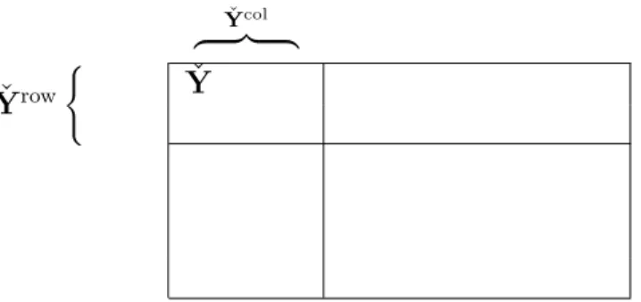
column blocks after cutting the forestogram by a plane. Forestogram projection on rows and on columns provides two marginal dendrograms. Forestogram side view (left panel), above view (middle panel), projec-tion of the forestogram on rows and columns resembling a heatmap graphics (right panel) ; the dotted horizontal and vertical lines is the projection of the cutting plane. . . 29 Figure 4.3 Visual illustration of submatrix ˇY ⊂ Y, extended on rows ˇYrow, and
on columns ˇYcol. . . . 33 Figure 4.4 Notation for a separable bicluster ˇY ⊂ Y. . . . 34 Figure 4.5 Time required to build the forestogram as the number of rows n increase
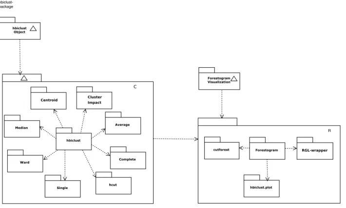
(top panels), and as the number of columns p increase (bottom panels). The top right panel confirms that the algorithm is quadratic in n, the bottom right panel confirms that the algorithm is quadratic in p ; the solid line is y = β0+ 2x. . . . 37 Figure 4.6 R-package architecture consists of two components, the engine is
im-plemented in C, and the interface is developed in R based on the RGL library. . . 39 Figure 4.7 Symmetric simulation data consist of a matrix of size 30 × 30 with 9
biclusters. Each bicluster contains 100 data from uniform distribution with 10 rows in row cluster and 10 columns in column clusters. The parameter ∆ controls the separability of biclusters. . . 41
Figure 4.8 Top panel: forestogram produced using Ward bilinkage with automatic cut using FORIC. Bottom panel: two-dimensional projection of
fores-togram on rows and columns. . . 44
Figure 5.1 Result of the Semi-Circle Projection on the synthetic dataset from Table 5.1 in three dimension which illustrates how similar users are located close to each other. . . 60
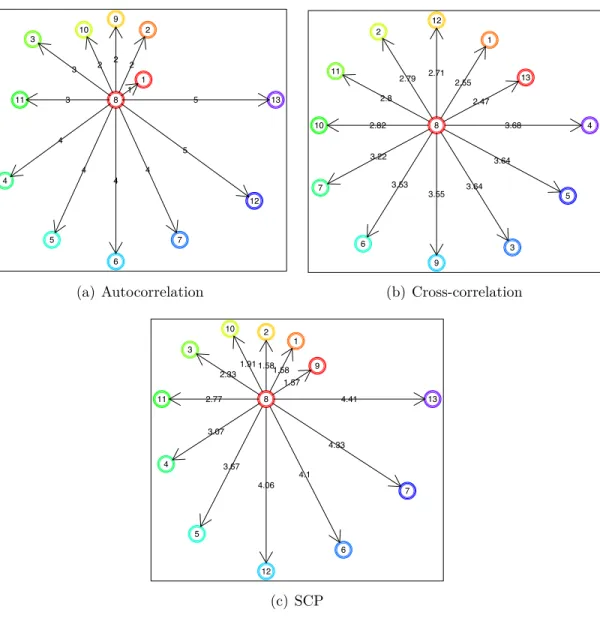
Figure 5.2 Comparison of the nearest users of X1 with three similarity measu-rements, autocorrelation, cross-correlation, and semi-circle projection, respectively. As we expect, observations show that SCP method effecti-vely sort out the similar users according to the temporal usage related to the user 1. . . 61
Figure 5.3 Comparison of the nearest users of X8 with three measures of similarity, autocorrelation, cross-correlation, and semi-circle projection, respecti-vely. As it could be seen, SCP is able to find out the analogous users by projecting them into three dimensions. . . 62
Figure 5.4 Histogram of the frequency of the traveled days in one month. . . 63
Figure 5.5 3D histogram of the overlapped projected data on xy-plane. . . . 64
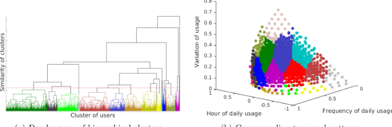
Figure 5.6 Dendrogram of the hierarchical clustering with the associated clusters of the projected data. Figure 5.6(a), shows 18 clusters, the total tem-poral patterns that exist for the one month period of the smart card usage. These clusters are shown on the projected data, in Figure 5.6(b). 66 Figure 5.7 Pattern of single trips ordered by early to late. . . 66
Figure 5.8 Pattern of regular users. . . 67
Figure 5.9 Patterns of late commuters. . . 67
Figure 5.10 Patterns of long-day trips vs midday excursion. . . 67
Figure 5.11 Patterns of active users versus inactive cards. . . 68
Figure 5.12 Distribution of clusters shown in Figure 5.6 for usual working days and weekends. . . 68
Figure 5.13 Daily cluster distribution for the entire period of the month. . . 69
Figure 5.14 A typical network of public transport . . . 71
Figure 5.15 Three users with the same start point and end point . . . 71
Figure 5.16 Two users taking the same buses in opposite directions . . . 71
Figure 5.17 Two users with the same directional pattern . . . 72
Figure 5.18 Two users with the same symmetric directional pattern . . . 72
Figure 5.19 Two users with the same pattern of usage except one . . . 72
Figure 5.21 The same resultant traversed distance with different bus stops . . . . 74 Figure 5.22 Two users taking the same buses with different order . . . 74 Figure 5.23 The same pattern of two users living in the different places . . . 74 Figure 5.24 User similarity based on circular grid representation of bus stops . . . 75 Figure 5.25 Pairwise bus stop difference criterion for measure of user similarity . 76 Figure 5.26 Visualization of the synthetic example of spatial-temporal data
asso-ciated with 8 users and the corresponding spatial usages during 5 hours shown in Table 5.2. . . 78 Figure 5.27 Forestogram of the synthetic example of spatial-temporal data defined
in Table 5.2. . . 79 Figure 5.28 Forestogram built on top of the cluster centers obtained from the real
data. . . 80 Figure 5.29 Patterns of spatial-temporal behavior extracted from the real data with
modified forestogram. x axis encodes the discrete hourly usages and y axis shows the shared location in (latitude, longitude) pair. . . 81 Figure 5.30 Patterns of spatial-temporal behavior extracted from the real data with
modified forestogram. x axis encodes the discrete hourly usages and y axis shows the shared location in (latitude, longitude) pair. . . 82 Figure 5.31 Patterns of spatial-temporal behavior extracted from the real data with
modified forestogram cont. x axis encodes the discrete hourly usages and y axis shows the shared location in (latitude, longitude) pair. . . 83 Figure 6.1 Integrative model for combining seven multiomics dataset through
cross-validation. In the first layer, for each omic dataset a regression model is tuned. Then the integrative prediction is made by bringing gestational output from each omic dataset together in the second layer. . . 87 Figure 6.2 (a) Overview of the study design. A total of 51 samples are
collec-ted during three trimesters of pregnancy as well as an addition 17 samples 6 weeks after delivery. Seven datasets are produced for each sample. (b) The number of biological measurements in each dataset. (c) Complexity of each dataset calculated as the number of principle components needed to capture 90% variance. . . 88
Figure 6.3 a) Overview of the two-layer cross-validation procedure. On the ou-ter layer, a modified leave-one-patient-out cross-validation procedure is used in which all samples from the same subject (as opposed to just one subject) is left out as a blinded sample. Within each fold a second cross-validation is performed to optimize the free parameters of elas-tic net. (b and c) the Spearman correlation between the (b) training set and (c) test set cross-validated results for each dataset. (d) perfor-mance of the trained models on the whole datasets including the first trimesters of pregnancy and post-partum that is never exposed to the training set. . . 90 Figure 6.4 (a) Stacked generalization analysis. The size of the boxes is
propor-tional to the log 10 of the number of measurements in each dataset. The thickness of the arrow is proportional to the − log10 of p-value of a correlation test for gestational age ; (b) Visualization of the most predictive features in a correlation network. The size of each node is proportional to the univariate correlation between that feature and gestational age. Color represents the corresponding dataset. . . 92 Figure 6.5 An example of bivariate elastic net penalty with α = .5, in presence of
LASSO and ridge regression constraints. . . 95 Figure 6.6 Ablation (left) and inverse ablation (right) analysis of each dataset’s
contribution in the integrative model. Elimination of each dataset is carried out according to the p-value of gestational age prediction shown in Figure 6.4 in ascending, and descending order, respectively. Color portion is associated with the coefficient of each dataset represented by the stacked generalization integrative model. . . 97 Figure 6.7 Correlation network of interrelated features extracted from different
multiomics dataset. An edge reflects the adjusted correlation among the multiomics features. A node’s size represents the magnitude of the corresponding elastic net coefficient. Correlation direction is denoted by the intensity of blue and red colors indicating the negative or positive correlation, respectively. . . 99 Figure 6.8 Regression lines between actual gestational age and the corresponding
predictions from seven multiomics dataset and stacked generalization with their 95% confidence interval. . . 100
Figure 6.9 Regression lines between actual gestational age and the corresponding predictions from seven multiomics dataset and stacked generalization with their 95% confidence interval cont. . . 101 Figure 6.10 Overview of performance comparison using a number of regression
al-gorithms, e.g. random forest, XGboost, Gaussian process, support vec-tor regression, and elastic net. The hyper parameters of each method are tuned by the two-layer leave-one-patient-out cross-validation pro-cedure for predicting the gestational age on the test set. Elastic net predominantly outperforms the other rival methods especially for the integrative model. . . 102 Figure 6.11 Illustration of rank correlation among a number of datasets. Left panel
shows the network representation of RGCCA after Bonferroni adjust-ment such that presence of an edge between a pair of nodes shows strong correlation between those nodes. Right panel simply demonstrates the heatmap visualization of correlation among two datasets. . . 103 Figure 6.12 Illustration of rank correlation among a number of datasets cont. Left
panel shows the network representation of RGCCA after Bonferroni ad-justment such that presence of an edge between a pair of nodes shows strong correlation between those nodes. Right panel simply demons-trates the heatmap visualization of correlation among two datasets. . 104 Figure 6.13 Unsupervised RGCCA performance on the seven multiomics dataset.
Since Serum and Plasma generated from Luminex family are the most similar omics, they are grouped in one cluster. The remaining datasets show more consistency by forming another tangible cluster. . . 106 Figure 6.14 Unsupervised integrative model through forestogram biclustering on
the features of multiomics dataset. . . 108 Figure 6.15 Hierarchical biclustering integrative model shown on heatmap. . . 109
LIST OF NOTATIONS AND ACRONYMS
NOTATIONS:
Ci biclusters i
n number of subjects, or number of rows
p number of attributes, or number of columns
Yn×p n × p data matrix
ˇ
Y submatrix of Y, i.e. ˇY ⊂ Yn×p
¯
y(.) mean of cluster
˜
y(.) median of cluster
σ2 common within variance
φ between to within variance ratio
s2 pooled variance
M(.) margin of bicluster
D(.) diameter of bicluster
D(., .) dissimilarity measure between a pair of biclusters
Si spatial usage of card i
Xi binary temporal usage of card i
ri temporal boarding radius of card i
θi temporal boarding angle of card i
zi temporal boarding variance of card i
Hadamard (elementwise) product operator
||.|| Euclidean norm
|c| absolute value of the scalar c |C| cardinality of the set C
ACRONYMS:
AIC Akaike Information Criterion BIC Bayesian Information Criterion
DBSCAN Density-Based Spatial Clustering of Application with Noise
DTW Dynamic Time Warping
EDM Euclidean Distance Matrix FORIC FORest Information Criterion GIS Geographic Information System
MST Minimum Spanning Tree
NMF Nonnegative Matrix Factorization
RGCCA Regularized generalized canonical correlation analysis SCP Semi-Circle Projection
SCFCS Smart Card Fare Collection System STO Société de Transport de l’Outaouais
CHAPTER 1 INTRODUCTION
The rapid growth of data according to the progress of sensors and storage technologies has been emerging in several different areas (Jain, 2010). Various sources can generate these data, from the Internet search, digital videos, imaging and biological sequences to smart card data used in public transit. Therefore many researchers and scientists from miscellaneous fields such as mathematics, statistics, computer science, urban computing and planning, ma-nagement, business, civil engineering, industrial engineering, Geographic Information System (GIS), and biology have encouraged to concentrate on finding methods for grouping a set of data (Jain, 2010; Everitt et al., 2011). The main purpose of extracting similar groups of data without label information is to discover knowledge and interpret the high volume data before deep analyzing the fine-grained components that are hidden in the underlying data. In the most simplest way, clustering aims to ensure giving a coherent and complementary big picture of a complex dataset to figure out what one can do with the data where every-thing is intricate. In marketing, similar group of customers with similar commercial habits or demographic can be found by clustering (Murray et al., 2017; Huang et al., 2007; Punj and Stewart, 1983). In biology, grouping similar diseases, genes or phenotypes according to the different level of measurements is easily carried out by clustering (Nugent and Meila, 2010; Ben-Dor et al., 1999; Eisen et al., 1998; Eren et al., 2013). In public transport and city planning, clustering is used to identify similar users, passengers profiling, station grouping, and infrastructure development (Pelletier et al., 2011; Carel and Alquier, 2017; Nin et al., 2013; Galba et al., 2013; Vos and Witlox, 2013). Clustering has many other interesting ap-plications in digital domain, such as document retrieval, image segmentation, recommender systems, search engine, social networks, etc. (Orzechowski and Boryczko, 2016; Zamir and Etzioni, 1998; Huang, 2008; Pal and Pal, 1993). The formation of coherent data as a unit of cluster together could be carried out according to a measure of similarity which reflects the relationships among the data. Thus the increase of data generation, in both capacity and diversity, demands fundamental improvement in methodological and algorithmic methods toward spontaneously realizing, processing and extracting the patterns underlying the data. One of the most important and challenging tasks in machine learning, statistics and gene-rally data analysis is grouping similar objects together (Kleinberg, 2003; von Luxburg et al., 2012). In recent years, this task known as clustering, has arisen as a progressively impor-tant research topic both in theory and application such as pattern recognition, data mining, bioinformatics, computer vision, social network, etc. (Eisen et al., 1998; Madeira and Oli-veira, 2004; Orzechowski and Boryczko, 2016; Tu and Honavar, 2008; Jain, 2010). Clustering
analysis, due to the absence of the label information, is called unsupervised learning. Unlike the other existing problems in this field, such as, classification or regression, in the study of clustering analysis, there is no a priori knowledge available to identify the category label information for the given data.
Unlike confirmatory methods that deal with validating the given assumptions of the mo-del to the data, the purpose of exploratory methods, is to discover and extract groups of data, known as data clusters, into interpretable and meaningful information to the specia-lists (von Luxburg et al., 2012). Clustering is an exceptionally tough combinatorial problem that belongs to the NP-hard class of computational complexity problems (Ackerman and Ben-david, 2009). Indeed, it was shown that there is no clustering algorithm that is able to preserve certain properties for data clustering (Kleinberg, 2003). In this regime, clustering is more likely considered as an art rather than science (von Luxburg et al., 2012). To cope with this difficulty, quite many different techniques were already suggested in plenty of contexts by numerous researchers which demonstrate the broad necessity and appeal to the exploratory data analysis problem (Jain, 2010).
Usually, there is no right or wrong clusters. Because evaluating a clustering algorithm depends on why user does clustering and how the result of clustering can be used (von Luxburg et al., 2012). In the case of low-dimensional data (ideally less than 4) by plotting the data, we can distinguish the clusters in the data visually. However, recently, the advent of high-dimensional data demonstrates the need for devising new algorithms to reveal the clusters by exploring the data. Therefore, appropriate clustering criterion can be deployed to extract suitable clustering assignment from the data to meet users’ demand. Clustering algorithms are categorized into two groups: hierarchical and partitional (Jain, 2010). In the former category, hierarchical methods try to find nested clusters recursively, while in parti-tional approaches data are split into a non-overlapping division of subsets without any nested procedure. Hierarchical methods are being used widely in applied projects, especially for pu-blic transit (Patnaik et al., 2016; Wang and Yu, 2010) and bioinformatics (Pontes et al., 2015; Madeira and Oliveira, 2004). In order to address these applications successfully, one of the concerning questions that should be answered significantly is the estimation for the number of clusters. Consequently, the cutting point on the dendrogram at certain height to illustrate a set of major clusters existing in the hierarchical configuration has been a well-known problem for decades. The majority of algorithms for this regard can be divided into distance-based or model-based methods (Stahl and Sallis, 2012; Oh and Raftery, 2007; Farrar, 2006; Tan
et al., 2006; Izenman, 2008). Distance-based techniques are easy to understand and simple to
implement. On the contrary, model-based approaches are flexible and adapt to data pattern, but are counter intuitive to implement. However some methods are developed for
distance-based methods using cross validation (Tibshirani et al., 2001), or for model-distance-based methods using statistical asymptotic (Claeskens and Hjort, 2008). Our suggestion is to apply a simple Bayesian hierarchical model that allows to apply the ratio of posterior predictive (Kass and Raftery, 1995), as the standard model selection criteria. Hence, we develop a Model-based
Clustering that assumes a statistical model for clustering the data based on hierarchical
settings with promising results in real world applications (McLachlan et al., 2004).
Hierarchical clustering is a breakthrough in clustering, because of producing a visual
guide in the form of a binary tree, known as dendrogram. In addition, it requires little prior knowledge, except for a dissimilarity measure (Johnson, 1967; Sokal and Sneath, 1963). The dissimilarity measure is a positive semi-definite symmetric mapping of pairs of groups onto the set of real numbers (Murtagh and Legendre, 2014). This measure, however, may not sa-tisfy the triangle inequality unlike the distance (Murtagh and Legendre, 2014). Hierarchical algorithms require a dissimilarity measure to merge clusters in order to build a nested struc-ture of clusters. The common dissimilarities include single linkage (or nearest neighbors), complete linkage (or farthest neighbors), average linkage, and centroid linkage (Murtagh and Legendre, 2014) among others. There are two variants of hierarchical clustering methods de-pending on the direction of the construction of the nested groups. Agglomerative clustering starts with every observation as a singleton and consequently merges the closest clusters to end up with all data in one cluster (Johnson, 1967). Divisive algorithms, on the contrary, starts with all data in one cluster and splits the clusters until finishing with all singletons (Everitt et al., 2011).
Clustering could be applied on public transit domain where everyday, thousands of people travel (de Oña and de Oña, 2015; Ghasemzadeh et al., 2014; Hasan et al., 2012; Fuse et al., 2012). Each time a smart card is tapped on the card reader, plenty of information is gathered that possibly could lead analysts, engineers, managers and strategists to excavate, design, decide, and plan more effectively based on the users behavior in this network (Dou et al., 2015; Park et al., 2008; Kurauchi and Schmöcker, 2017; Pelletier et al., 2011). Investigating users behavior according to the data is a nontrivial task. It requires sophisticated mathematical, statistical, data mining and machine learning techniques to exploit the hidden patterns of the stored data. Such data is dynamic and rigorously increasing because of population growth and development of infrastructure. Moreover, affordable cost of public transit in comparison to private car, especially, in the large cities, metropolitan areas and their suburb increases the daily usage of this network. In this regard, we propose new methods of spatial-temporal data analysis to investigate patterns of user’s behavior in public transit.
The importance of the public transportation and its influence in the real life of many people in large cities around the world rises a new family of problems that is not confined
into a particular branch of science (Weisbrod and Reno, 2009). Hence, usage of the smart card data creates the opportunity for several different researchers from diverse disciplines e.g. data mining, machine learning, urban computing and planning, management, business, civil engineering, industrial engineering, statistics, mathematical engineering, GIS, etc. to outreach and extend their methods to analyze the data for the public transport authorities (Weisbrod and Reno, 2009; Gallotti and Barthelemy, 2015; Fuse et al., 2012; Ortega-Tong, 2013; Lathia et al., 2010).
Despite extensive researches have been done on public transportation domain, various obstacles have been arisen for specific purposes which require particular approaches to address them. In this study, a recent problem of clustering the similar users is introducing according to the spatial-temporal data gathered from smart cards to analyze the user’s behavior in the public transport network.
Smart card data, contains worthwhile digital information of daily locations visited at certain period of a large number of individuals. The wealth of collected data down to a single time, and location resolution creates fundamental challenges that require a mix of analytical, algorithmic, and statistical techniques (Pelletier et al., 2011). Beside other sources of information such as mobile phone, GPS tracker vehicle, e.g. bike, car, motorcycle, credit card transactions, social network, and many other sources of information gathering, smart card data is the best promising source of users digital information (Hasan et al., 2012). Thus this helpful information could be utilized to characterize and model urban mobility patterns (Hasan et al., 2012). Other useful information such as travel time and number of passengers for the sake of congestion analysis and planning improvement, could be possibly extracted as well (Fuse et al., 2012).
From a different perspective, high-throughput technologies such as cell-free RNA, plasma luminex, serum luminex, immune system, metabolomics, and plasma somalogic have been recently studied for different biological researches e.g. aging, recovering from surgery, stroke, pregnancy, cancer, etc. in order to provide statistical predictive models for diagnosis, prog-nosis and therapy (Clarke et al., 2008; Yau et al., 2016; Dey et al., 2017; Ji and Liu, 2010). Every single biological dataset consists of hundreds or thousands of highly correlated mea-surements for each sample so that extracting meaningful biological information from these high-dimensional datasets through statistical techniques delivers tremendous insights for bio-logical investigators (Schwenk et al., 2010; Bendall et al., 2011; Kang et al., 2008; Sreekumar
et al., 2009; Miyagi et al., 2010; Katz et al., 2016; Romero et al., 2017; Clarke et al., 2008).
Devising, designing and implementing statistical data analysis methods make the biologists better comprehending the role of certain group of genes, proteins, and many other biological measurements intuitively to address the critical questions in drug development, treatment
strategy, gene signaling pathway, etc (Miller et al., 2008). Toward the goal of making the sense of data for biologists, visualization plays a central role especially for displaying hierar-chical structures. Hierarhierar-chical clustering and its applications are familiar to many biologists so that pairwise relationships between data points are represented by a rooted binary tree. This kind of clustering is widely used for evolutionary analysis of sequence history e.g. phylo-genetic sequencing, gene expression patterns, DNA microarray expression, etc. (Eisen et al., 1998; Clarke et al., 2008; Miller et al., 2008; Xu and Wunsch, 2005). Intuitive illustration of groups without complicated assumptions about the intrinsic of the data distribution, along with the effective computational complexity make the hierarchical approach the first choice for analyzing biological data (Eisen et al., 1998).
The main goal of this thesis is the development of forestogram framework for hierarchical biclustering with the applications in public transit and bioinformatics. In practical applica-tions, a method that is easy to understand by people is desirable. Hierarchical clustering is an intuitive method of clustering for many people in industrial engineering and bioinforma-tics. Additionally, binary tree representation known as dendrogram is easy to elaborate the result such that the result interpretation is easy enough to provide a descriptive summary of the data. In public transit domain, we often deal with two types of distinct information, temporal and spatial. For the temporal data that are similar to time series data, the hie-rarchical clustering techniques are not suitable because off-the-shelf distance metrics are not designed for binary vectors. To this end, we first suggest a projection technique to map a long binary vector of temporal usage into three dimensional space which retains the proximity of pairwise similarity. For the next step, we take the temporal information as a latent variable to extract the spatial-temporal patterns from the data such that Euclidean metric becomes feasible because of geodesic property of GPS location history. In the context of multiomics analysis of gestational age prediction, we suggest to analyze each dataset separately to show how each biological measurement is influencing the term of pregnancy. For the integrative model, we suggest the stacked generalization and forestogram approaches for supervised and unsupervised integrative data analysis.
In Chapter 4, we address the biclustering problem in general and as an extension to the idea of model-based hierarchical clustering in particular where we have a matrix that consists of rows and columns such that grouping of both sides is the case of interest. This is a variant of normal grouping of data but instead of only similar groups of samples, a block of submatrix with subjects that are highly correlated with features forms the biclusters. Analogous to the conventional linkages for hierarchical clustering, we suggest a bilinkage dissimilarity measure for constructing a hierarchical setting for these biclusters. Consequently, we also develop forestogram visualization technique similar to dendrogram with one extra
dimension to emphasize the direction of the merge when switches from row to column or vice-versa. Then we elaborate how to find the number of representative biclusters on the forestogram by making a subtle connection from hierarchical fashion to the model based setting. This way, Bayesian viewpoint helps us estimating this number by deploying FORIC that is a kind of information criterion trick motivated by Bayesian Information Criterion (BIC). Then this framework is tested on synthesized, plus real world instances such as public transit, and biological datasets. Promising results from simulation and empirical studies turn out that forestogram outperforms almost all rival techniques comparing with histogram and a number of similar methods.
In Chapter 5, first we introduce a temporal projection that maps a high-dimensional binary vector corresponding to the hourly usage of public transit into a space of three di-mension with a semi-circle shape. This ad-hoc projection is exclusively designed to mimic the clock as a clue for temporal data with a number of interesting mathematical properties that retains the similar users close by. Despite many metrics defined for computing the distance between an arbitrary pair of data, such as Euclidean, Manhattan, Hamming, etc. none of them satisfies the relations for temporal binary vectors. To this end, our suggested projection meets certain properties that are suitable for analyzing the temporal public transit data. One of the most interesting advantages is the visualization scheme so that makes it easy for trans-port analysts to better understand how a hierarchical clustering model works on top of this projection. Furthermore, adding the spatial data which represents the geographical location history for associated time-points, enables the modified version of forestogram to specify the spatial-temporal user behavior through the standard Euclidean metric. These methodologies are inspired by the Société de transport de l’Outaouais data with successful results that are present in the experiment section.
Chapter 6, is devoted to the integrative clock of human pregnancy in three trimesters before delivery and postpartum with seven multiomics measurements to investigate the level of changes in these datasets over the term of pregnancy. The goal of this study is to find si-gnificant features that are correlated with gestational age in three trimesters before delivery. We develop an algorithm which determines the significant correlated features leading the gestational age on each dataset apart at first step, then an integrative step is implemented in two different levels, features pool and predictions stack. In the feature level, all datasets together make a holistic model for all patients, while the stack generalization outlook takes the independent predictions from each single dataset as a new feature to predict the gesta-tional age. Moreover, due to the ethnicity and particular specifications of women, different features could affect certain patients toward predicting the gestational age. We compare the performance of forestogram as an unsupervised biclustering technique with the elastic net
(Zou and Hastie, 2005) as a supervised variable selection regression method to figure out how much supervised information is necessary toward predicting the trimesters of gestational age in addition to the important features that are correlated with the clock of pregnancy.
CHAPTER 2 LITERATURE REVIEW
2.1 Hierarchical Clustering
The number of ways for partitioning a set to examine all possible clustering increases ex-ponentially in terms of the number of data points and grouping. In this regard, hierarchical clustering algorithms are designed to discover the underlying clusters in a given dataset effi-ciently. Looking for a reasonable setting of clusters without refining all possible combinatorial assignments is made possible through hierarchical algorithms (Rencher, 1998).
Agglomerative hierarchical clustering consists of a bottom-up sequential process so that the number of clusters shrinks by starting from all singleton clusters whereas the volume of clusters grows gradually by ending up in one cluster surrounding all. In contrast, top-down divisive approach is the opposite viewpoint where a single cluster contains all data points in the beginning then splits into two groups in the next step. The end result of the divisive method is exactly the same as the start point of the agglomerative algorithm (Everitt et al., 2011). For better understanding the mechanism of constructing a dendrogram as a visualization technique for hierarchical clustering, an example is shown in Figure 2.2 where two separable classes of univariate data are given in Figure 2.1.
Figure 2.1 A univariate example of 5 data points.
In Figure 2.2 a simple example is shown where in the beginning, we have 5 clusters such that every single data point constitutes the finest clusters (each data point is a singleton cluster) see Figure 2.2(a). As it could be seen in Figure 2.2(b), data A and B are the most proximate pair of data that are agglomeratively combined together to create a new cluster at this step. Then, data point C joins the newly formed cluster, i.e. (A, B) as the closest cluster among the remaining ones in Figure 2.2(c). In the next step in Figure 2.2(d), (D, E) pair are merged together to form a new cluster. Then eventually, after combination of (D, E) to ((A, B), C) we get the coarsest cluster to the given set (all data points in one cluster).
Bottom-up approach is easy to form the hierarchy of clusters based on a dissimilarity measure in comparison to top-down method which requires a priori knowledge about the structure and shape of clusters. Having little prior knowledge, except for the dissimilarity
(a) (b)
(c) (d)
Figure 2.2 Step by step demonstration of agglomerative hierarchical clustering.
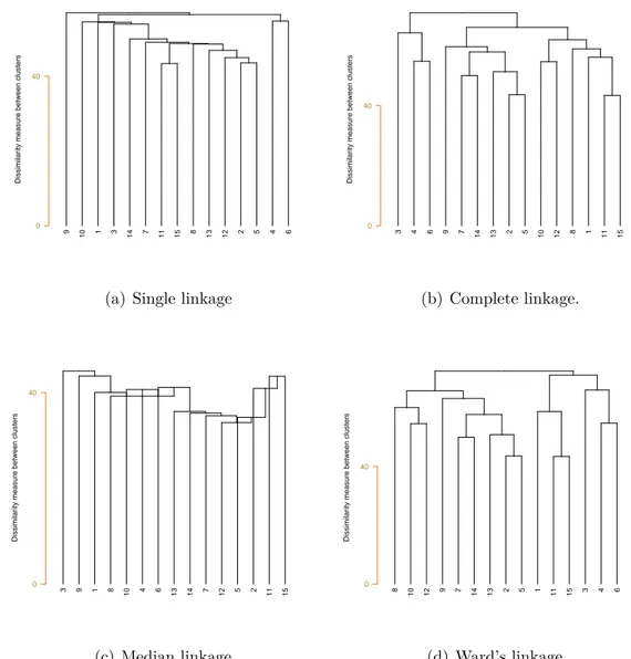
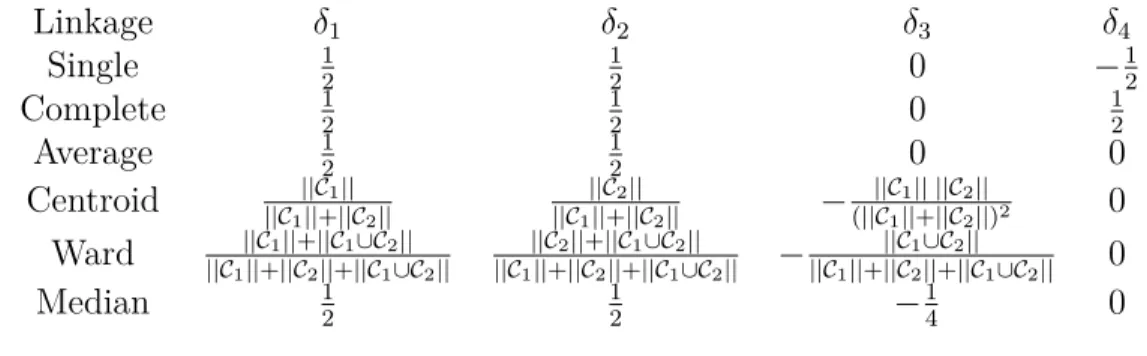
measure is one of the advantages of hierarchical clustering algorithms. The dissimilarity measure is a positive semi-definite symmetric mapping of pairs of groups onto the set of real numbers. This measure, however, may not satisfy the triangle inequality unlike the distance. The common dissimilarity measures include, single linkage or nearest neighbours (Florek et al., 1951; Sneath, 1957; Johnson, 1967), complete linkage or farthest neighbours (Sørensen, 1948), average linkage (Sokal, 1958), centroid linkage (Eisen et al., 1998), median linkage, and Ward’s linkage or minimum variance (Murtagh and Legendre, 2014).
In Chapter 4 we extend the definition of dissimilarity measure in the form of bilinkage such that the hierarchical biclustering can be constructed to illustrate the nested structure
of block-clusters by the associated forestogram. Apart from a pair of biclusters with dissimi-larity measure that should be merged together, direction of the merge is also necessary for forestogram to show how a pair of block-clusters is correlated.
Here we briefly introduce the existing linkages for hierarchical clustering so that bilinkage can be define respectively. In the following notation, yi ∈ Rprepresents a data point belonging
to a certain cluster, d(yi, yj) is the Euclidean distance, then the squared Euclidean distance
using norm ||.|| can be defined as d2(y
i, yj) = ||yi− yj||2 =Ppk=1(yik− yjk)2, and ||Ci|| refers
to the number of data points in the cluster Ci. Figure 2.3 elaborates the role of each linkage
on a random dataset. 2.1.1 Single Linkage
Early single linkage, also known as the nearest neighbor clustering, is one of the oldest and most famous of the hierarchical techniques that is developed by (Florek et al., 1951; Sneath, 1957; Johnson, 1967) which assumes no cluster shape to produce more dense, and chain-like clusters. Single linkage tends to merge close data points or singleton clusters together due to the early merge of two partitions ; this undesired property is known as chaining effect see Figure 2.3(a). In other words, a chain of singleton clusters can be extended for long distances against the general form of the cluster. In the single linkage, the distance between two disjoint clusters C1 and C2 is defined as,
Dsingle(C1, C2) = min
yi∈C1,yj∈C2
d(yi, yj)
2.1.2 Complete Linkage
Complete linkage, also known as furthest neighbor or maximum method, is initiated by Sørensen (1948) that roughly produces clusters with almost equal diameters. Complete linkage suffers from the opposite drawback of single linkage problem. If data contains outliers the complete linkage may not combine two proximate clusters in the appropriate order of merge in the hierarchical path see Figure 2.3(b). In the complete linkage, the distance between two disjoint clusters C1 and C2 is defined as,
Dcomplete(C1, C2) = max
yi∈C1,yj∈C2
d(yi, yj)
2.1.3 Average Linkage
Average linkage, also called the weighted pair-group method, is suggested as a trivial compromise between the single linkage and the complete linkage in Sokal (1958). Average
linkage prefers combining clusters with small variances that can be figured out as clusters with the same variance (Sokal, 1958). In the average linkage, the distance between two disjoint clusters C1 and C2 is defined as,
Daverage(C1, C2) = 1 |C1| |C2| X yi∈C1 X yj∈C2 d(yi, yj) 2.1.4 Ward Linkage
Ward’s linkage minimizes the total within-cluster variance by a weighted squared distance between cluster centers. Ward’s method merges clusters to maximize the likelihood at each iteration where spherical covariance matrices is deemed see Figure 2.3(d). Merging pair of clusters with few samples is what preferred by Ward’s method to generate balanced size clusters (Milligan, 1980). In the Ward’s linkage, the distance between two disjoint clusters C1 and C2 is defined as,
DWard(C1, C2) = X yi∈C1∪C2 ||yi− ¯y(C1∪ C2)||2− X yi∈C1 ||yi− ¯y(C1)||2− X yi∈C2 ||yi− ¯y(C2)||2 = |C1| |C2| |C1| + |C2| ||¯y(C1) − ¯y(C2)||2
where ¯y(C1) and ¯y(C2) are the mean vectors of clusters C1 and C2, respectively. 2.1.5 Centroid Linkage
Centroid linkage, also referred to as the unweighted pair-group centroid method, simply minimizes the squared Euclidean distance between cluster means and is less sensitive to outliers in comparison to the other linkages (Milligan, 1980). In the centroid linkage, the distance between two disjoint clusters C1 and C2 is defined as,
Dcentroid(C1, C2) = ||¯y(C1) − ¯y(C2)||2 2.1.6 Median Linkage
Median linkage, also called the weighted pair-group centroid method, is a variation on centroid linkage which defines the distance between two clusters as the weighted distance between their centroids. This weight is corresponding in size to the number of samples in each cluster. This method is only used with Euclidean distance. This linkage can be used for downweighting the effect of outliers by using the median instead of the mean see Figure
2.3(c). In the median linkage, the distance between two disjoint clusters C1 and C2 is defined as,
Dmedian(C1, C2) = ||˜y(C1) − ˜y(C2)||2
where ˜y(C1) and ˜y(C2) are the medians of clusters C1 and C2, respectively.
Dissimilar
ity measure betw
een clusters
9 10 1 3 14 7 11 15 8 13 12 2 5 4 6
0 40
(a) Single linkage
Dissimilar
ity measure betw
een clusters 3 4 6 9 7 14 13 2 5 10 12 8 1 11 15 0 40 (b) Complete linkage. Dissimilar
ity measure betw
een clusters 3 9 1 8 10 4 6 13 14 7 12 5 2 11 15 0 40 (c) Median linkage. Dissimilar
ity measure betw
een clusters
8 10 12 9 7 14 13 2 5 1 11 15 3 4 6
0 40
(d) Ward’s linkage.
Figure 2.3 Dendrograms corresponding to the four different linkages in hierarchical clustering applied to random data. As it is shown in Figure 2.3(c) monotonicity property is not satisfied for all linkages.
2.1.7 Properties of hierarchical algorithms
Properties of hierarchical algorithms are usually expressed as (i) Lance-Williams, (ii) Mo-notonicity, and (iii) Space Distortion (conserving, contraction, or dilating) (Rencher, 1998). Lance-Williams property is discussed with more details in Chapter 4 with its extension for forestogram framework.
Monotonicity property of clustering states that a cluster is not allowed to get merged with another cluster at a height that is less than the height of the previously combined clusters. This also is referred to as ultrametric which inspires the separability assumption for our developed forestogram in the context of extended hierarchical algorithms for biclustering. In Figure 2.3(c) median linkage as an example of nonmonotonic is shown, similarly with a counter example one can demonstrate centroid is not monotonic either.
Properties of the space of distances can change after creation of clusters. Clustering al-gorithm is space-conserving if the spatial properties always stay intact, otherwise the space can be either contract or dilate in the sense of changes occur to the distances between any arbitrary pair of data points. The tendency of a singleton clusters to join the newly crea-ted cluster is called contraction, while the opposite behavior is known as dilating. In space contracting algorithms, larger clusters frequently appear after each merge, so that singletons eventually combine with non-singleton large clusters. For the space-dilating algorithms we expect to have more new clusters rather chaining property (Rencher, 1998). In this fashion, singleton clusters are more likely to join the other singleton clusters rather than with non-singleton ones. Let’s consider three clusters, Ci, i ∈ {1, 2, 3}, where the pairwise distances are
defined as,
D(C1, C2) < D(C1, C3) < D(C2, C3) (2.1) If the equation in (2.1) is not held, the clustering algorithm is space-contracting. Space-conserving algorithm does meet the conditions in equation (2.2).
D(C1, C3) < D(C{1,2}, C3) < D(C2, C3) (2.2) And space-dilating algorithm does not satisfy the equation (2.2).
The hierarchical algorithm with single linkage is prone to space-contracting tendency be-cause of violating the first inequality D(C{1,2}, C3) = min {D(C1, C3), D(C2, C3)} = D(C1, C3), therefore single linkage is not preferred in many fields see Figure 2.3(a). On the other hand, complete linkage is in the class of space-dilating algorithms because of violation of the second inequality D(C{1,2}, C3) = max {D(C1, C3), D(C2, C3)} = D(C2, C3) correspondingly new clus-ters are more likely to be seen at each iteration see Figure 2.3(b). Other hierarchical linkages are often somewhere in between single linkage and complete linkage, e.g. centroid linkage and
average linkage algorithms are more biased to space-conserving, however Ward’s linkage is in favor of space-contracting see Figure 2.3(d) (Rencher, 1998). The mentioned space properties provide a clue for considering how likely a dendrogram one can expect in terms of balanced or unbalanced group of homogeneous data.
Furthermore, stability and convergence of hierarchical clustering algorithms are discussed in Carlsson and Mémoli (2010). Hartigan consistency is reviewed in Eldridge et al. (2015) as a framework for analysing the hierarchical clustering. Then merge distortion metric is suggested in order to alleviate the over-segmentation and improper nesting with two limited properties, separation and minimality (Eldridge et al., 2015).
2.1.8 Model-based cluster estimation
The majority of clustering algorithms can be divided into distance-based methods or model-based methods. Distance-based techniques are easy to understand and simple to im-plement. On the contrary, model-based approaches are flexible and adapt to complex data patterns, but are counter intuitive to implement. In model-based clustering a family of sta-tistical models is considered for data. Estimating the number of clusters in both approaches is a complex problem. However, some methods are developed for distance-based methods using cross validation (Tibshirani et al., 2001), or often asymptotic model selection criteria is used (Claeskens and Hjort, 2008). Estimating the number of clusters through cutting the dendrogram at certain height, is equivalent to find a tangible gap on the height of the dendro-gram for a natural grouping. An approximate model selection criteria such as AIC (Akaike, 1973) or BIC (Schwarz, 1978) can be applied to cut the dendrogram if a statistical model is used to produce the nested clusters (Heller and Ghahramani, 2005; Heard et al., 2006). We further extend the idea of model-based cluster estimation in Chapter 4, for finding the number of biclusters on our suggested forestogram. We suggest a model selection method which finds the cutting point of the forestogram automatically. In order to achieve this goal, suppose that θ is the associated parameter of the clusters. It turns out that f (y|θ) is the likelihood of the data if θ was known exactly. As far as, θ has not yet known, and grouping of the data is our main concern rather than the value of θ, the predictive distribution of the data can contribute to find the optimal cluster assignments. The solution of this predictive distribution is computed by marginalizing the likelihood of the data multiplied by prior dis-tribution of θ over the clustering parameter, i.e. p(y) = R
f (y|θ)f (θ)dθ. This resembles a
BIC criterion whose optimal number of clusters is found by computing it over all levels of the tree on a given forestogram. The marginal provides a measure of a merge that is supported by the model if increases for that merge. This way forestogram can decide how to cut the forestogram.
2.1.9 Biclustering
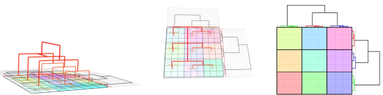
One of the desired goals in data analysis for an arbitrary multivariate dataset is to find barycentric relations for the hidden structure among subjects and their corresponding attri-butes (Govaert and Nadif, 2013). Finding the partitions of rows and columns at the same time is known as biclustering, however, in the literature is also referred to as two-mode clus-tering, coclusclus-tering, simultaneous clusclus-tering, two-way clusclus-tering, or two-side clusclus-tering, block clustering (Govaert and Nadif, 2013). Since the late 90s, biclustering has been the term most widely used in bioinformatics (Govaert and Nadif, 2013). The simple and easiest way for bi-clustering is to perform a bi-clustering algorithm to both sides, rows and columns independently to find the relevant blocks. Since for multivariate data analysis, columns of the matrix are generated from the samples located on the rows, independent clustering of rows and columns is not statistically significant for real world problems. After unfolding the relations among the correlated rows and columns, visualizing the simultaneous partitions is the next issue that should be addressed for biclustering problem. Heatmap is a conventional visualization method to display a matrix in terms of biclustering. Although heatmap applies hierarchical clustering on rows and columns independently, but it provides a good visualization scheme that is easy to understand. Independent dendrograms on row and column demonstrate a biclustering visualization where the intersection of row clusters in conjunction with that of column illustrates the structure of blocks underlying the data.
Despite the complicated nature of biclustering, this viewpoint to unsupervised partitio-ning has been arisen in many applied fields such as topic modeling in natural language processing whose goal is to extract the topics from the corpus of documents (Rugeles et al., 2017; Orzechowski and Boryczko, 2016), web mining to reveal the web pages that are vie-wed by certain group of people (Rathipriya and Thangavel, 2014), recommender system and marketing as a general class of problems where a shared behavior among group of people is the case of interest (Wang et al., 2015; Alqadah et al., 2015), bioinformatics to gene ex-pression profiling for molecular, cell or tissue in biological measurements (Eisen et al., 1998; Eren et al., 2013), manufacturing systems to show how the processing time and available machines as resources are interacting together (Boutsinas, 2013; Liiv, 2010), public transport for evaluating the most important roads in the network (Freiria et al., 2015; Owens, 2009) etc. Toward the meaningful biclustering viewpoint that aims at finding a block of correlated rows and columns, pairwise distance known as dissimilarity matrix plays a central role in classical approaches. The modern methods can be divided into three categories: (i) Bayesian approach: this perspective assumes a prior distribution over the statistical parameters of model (Gu and Liu, 2008; Martella et al., 2008; Zhang, 2010) ; (ii) Frequentist aspect: in this view the statistical model underlies fixed unknown parameters, such as mixture models (Lazzeroni and
Owen, 2002) ; and (iii) Matrix approximation view: this approach reconstructs the original matrix by multiplying two low-rank matrices where the first multiplicand and the second one reflect the cluster assignment of subjects and attributes, respectively (Donoho and Stodden, 2004; Ding et al., 2005; Arora et al., 2012; Wang and Zhang, 2013; Gillis, 2011; Klingenberg
et al., 2009; Cai et al., 2008; Lee and Seung, 2000).
Most of the biclustering algorithms are developed based on fixed number of biclusters that ask the user to manually gives this information to the algorithm. In many applications, determining the number of biclusters is another issue that needs to be handled by the algo-rithm itself. The pattern that biclustering algoalgo-rithm is seeking to find falls into three main categories namely, constant, additive and multiplicative. The pattern of equal values consti-tutes the constant model. If the rows and columns share an additive factor then the pattern is denoted by additive term, while the multiplicative model requires multiplicative factors to represent the bicluster pattern. Similarly, it is not hard to imagine a pattern that integrates these three different models to define the bicluster notion. From the statistical point of view, a pattern consisting of the correlation between rows and columns is preferred (Madeira and Oliveira, 2004). Since there is no concrete choice for defining a bicluster, the criterion for identifying a submatrix as a bicluster is problem dependent. In this regard, there is no al-gorithm that is able to detect all variations, thus for a particular problem or certain type of data, we need to design a new procedure to account for the required specifications. To this end, we design the forestogram framework for computing and visualizing the hierarchical bi-clustering introduced in Chapter 4 with successful results in two major fields (Ghaemi et al., 2017c). In the following, we go through the definition, specification, and goals of biclustering and related research works in public transport and bioinformatics.
2.2 Application
In a number of complex systems such as public transit network, biological sequencing and in general time series observations, similar groups are expressed in a nested hierarchical structure (Tumminello et al., 2010; Aghabozorgi et al., 2015). According to the intrinsic seasonal trend that repeats itself systematically over time, subclusters of homogeneous entities can be found in the underlying data up to a certain level. Moreover, often, in real world time series clustering analysis, determining the number of exact similar groups is a tough issue. For this reason, hierarchical approaches are one of the common choices for time series clustering in addition to the strength of visualization power in terms of binary dendrogram tree (Aghabozorgi et al., 2015; Van Wijk and Van Selow, 1999; chung Fu, 2011).
2.2.1 Public Transport
The importance of the public transportation and its influence in the real life of many people in large cities around the world, rises a new family of problems that is not confined into a particular branch of science. Hence, usage of the smart card data creates the opportunity for several different researchers from diverse disciplines e.g. data mining, machine learning, urban computing and planning, management, business, civil engineering, industrial engineering, statistics, mathematical engineering, geographic information system (GIS), etc. to outreach and extend their methods to analyze the data for the public transport authorities. Figure 5.14 shows a typical public transit network including users, buses, and subway lines.
Bus stop Subway station
Figure 2.4 A typical public transit network.
Despite extensive researches have been done on public transportation domain, various obstacles have been arisen for specific purposes which require particular approaches to address them. Here we review a recent concerning problem of clustering the transit users according to the spatial-temporal data gathered from smart cards to analyze their behavior in the public transit network.
Smart card data, contains worthwhile digital information of daily locations visited at certain period of a large number of individuals (Pelletier et al., 2011). Beside other sources of
information such as mobile phone, GPS tracker vehicle, e.g. bike, car, motorcycle, credit card transactions, social network, and many other sources of information gathering, smart card data is a promising source of users digital information. Thus, this helpful information could be utilized to characterize and model urban mobility patterns (Hasan et al., 2012). Other useful information such as travel time and number of passengers for the sake of congestion analysis and planning improvement, could be possibly extracted as well (Fuse et al., 2012).
Smart card data, usually provides two distinct information ; spatial and temporal (Pel-letier et al., 2011). Spatial data consists of coordinates of the bus stop e.g. latitude and longitude that could be GPS data or relative values. Temporal data describes the time each trip is taken, this information could be encoded in a 0 − 1 vector, where start of the trip is indicated by 1. According to these information, analyzing users behavior is divided into three categories, 1) Spatial patterns, 2) Temporal patterns and 3) Spatial-Temporal patterns.
1. In the first case, methods of analyzing spatial pattern, are taking the bus/subway stop’s information into account. It turns out measure of behavioral pattern only de-pends on the location of stops, taken by the users rather than having known the starting hour of their trip.
2. The second methods seek the information pertinent to the temporal data associated to the public transport usage. Consequently, computing user similarity score is carried out regardless of geographical information. The indices of 1 occurrences in the encoded vector, are playing the central role in this approach.
3. The third scenario, is a mixture of the spatial and the temporal data, called spatial-temporal data analysis to investigate users’ behavior. It could be viewed as a combina-tion of the last two steps or an independent approach to recognize the spatial-temporal behavioral pattern in the public transport domain.
Hierarchical algorithms have been used as an unprecedented clustering method on spatial-temporal public transit data, such as shared bicycle policy analysis (Lathia et al., 2012), traffic mining (Froehlich and Krumm, 2008), spatial-temporal clustering for congestion patterns detection in urban road network (Anbaroglu et al., 2014), rush hour motorcycle flow data analysis in Taipei City, Taiwan (Feng et al., 2014). Shirui (2016) uses hierarchical clustering for visual analysis of the spatial-temporal traffic flow patterns generated from transport hubs in Shanghai. Divisive analysis clustering is suggested for classification of large amount of speed data collected from GPS receiver in India (Patnaik et al., 2016). Hierarchical methods show successful result in extracting the temporal patterns from the trip data through the Beijing subway system to characterize individual passenger movement patterns (Xu et al., 2016).