Microscopic crowd simulation : evaluation and development of algorithms

HAL Id: tel-01420105

https://tel.archives-ouvertes.fr/tel-01420105

HAL is a multi-disciplinary open access archive for the deposit and dissemination of sci-entific research documents, whether they are pub-lished or not. The documents may come from teaching and research institutions in France or abroad, or from public or private research centers.

L’archive ouverte pluridisciplinaire HAL, est destinée au dépôt et à la diffusion de documents scientifiques de niveau recherche, publiés ou non, émanant des établissements d’enseignement et de recherche français ou étrangers, des laboratoires publics ou privés.

David Wolinski

To cite this version:

David Wolinski. Microscopic crowd simulation : evaluation and development of algorithms. Data Structures and Algorithms [cs.DS]. Université Rennes 1, 2016. English. �NNT : 2016REN1S036�. �tel-01420105�

ANN´EE 2016

pour le grade de

DOCTEUR DE L’UNIVERSIT´

E DE RENNES 1

Mention : Informatique

Ecole doctorale Matisse

pr´esent´ee par

David Wolinski

pr´epar´ee `a l’unit´e de recherche UMR 6074 IRISA

et au centre INRIA - Rennes Bretagne Atlantique

ISTIC

Microscopic Crowd

Simulation: Evaluation and

Development of Algorithms

Th`ese soutenue `a Rennes le 22 janvier 2016

devant le jury compos´e de :

Yiorgos Chrysanthou

Professeur, University of Cyprus / rapporteur

Pierre Degond

Professeur, Imperial College London / rapporteur

Ming Lin

Professeur, University of North Carolina / examinateur

Armin Seyfried

Professeur, J¨ulich Supercomputing Centre / examinateur

Kadi Bouatouch

Professeur, Universit´e de Rennes 1 / examinateur

Julien Pettr´e

Charg´e de recherche, Universit´e de Rennes 1 / directeur de th`ese

TH `

ESE / UNIVERSITE

´ DE RENNES 1

sous le sceau de l’Universite´ Bretagne Loire

Contents

List of Figures

List of Tables

1 Introduction

2 Background

2 Autonomous Agent-based Algorithms . . . 8

2.1 First-Order Algorithms . . . 8

2.2 Second-Order Algorithms . . . 9

2.2.1 Repulsive-Forces from Future Collisions . . . 9

2.2.2 Collision-Free Velocities . . . 10

2.2.3 Other Predictive Approaches . . . 11

2.3 Summary . . . 12

3 Centralized Algorithms . . . 13

3.1 Cellular Automata . . . 13

3.2 Data-Driven Algorithms . . . 14

3.3 Tiles and Patches . . . 16

3.4 Macroscopic Algorithms . . . 18

4 Conclusion . . . 20

3 Craal: Parameter Estimation and Comparative Evaluation of

Crowd Simulations

3.2.1 Microscopic Data Metrics . . . 29

3.3.1 Greedy approach (G). . . 30

3.3.2 Simulated annealing (SA) . . . 30

3.3.3 Genetic algorithm (GA) . . . 30

3.3.4 Covariance Matrix Adapation (CMA) . . . 30

4 Results . . . 31 4.1 Data Categories . . . 31 4.1.1 Microscopic data. . . 31 4.1.2 Macroscopic data . . . 33 4.1.3 Sketch-like data . . . 35 4.2 Benchmarks . . . 35

5 Analysis and Conclusions. . . 39

4 WarpDriver: Context-Aware Probabilistic Motion Prediction for

Crowd Simulation

2 Summary of Related Work . . . 45

3 Overview . . . 47

4 Notations and Setup . . . 48

5 Perception: collision probability Fields . . . 49

5.1 The Intrinsic Field . . . 50

5.2 Warp Operators . . . 50

5.2.1 Agent-Related Operators . . . 50

5.2.2 Context-Related Operators . . . 51

5.2.3 Composition of Warp Operators . . . 52

5.3 Combining collision probability Fields . . . 53

6 Solving the Collision-Avoidance Problem . . . 53

7 Results . . . 54

7.1 Large and Dense Cases . . . 54

7.1.1 Test case 1: Big Groups . . . 55

7.1.2 Test case 2: Crossing . . . 55

7.1.3 Analysis . . . 55

7.2 Non-Linear Scenarios . . . 57

7.2.1 Test case 3: Curved Flows . . . 57

7.2.2 Test case 4: Curved Obstacle . . . 58

7.2.3 Analysis . . . 59

7.3 History-based Anticipation. . . 59

7.3.1 Test case 5: Zig-Zags . . . 60

7.3.2 Test case 6: Danger Corridor . . . 60

7.3.3 Analysis . . . 61

7.4 Highly-constrained Case . . . 63

7.4.1 Test case 7: Plane . . . 63

7.4.2 Analysis . . . 64

7.5 Benchmarks . . . 64

8 Discussion and Limitations . . . 65

CONTENTS

5 Applications to Evaluation and Parameter Estimation

1 Application to Insect Simulation . . . 71

1.1 Introduction . . . 71

1.1.1 Working Arrangements . . . 72

1.2 Related Work. . . 72

1.2.1 Graphics Point of View . . . 73

1.2.2 Biology Point of View . . . 73

1.2.3 Discussion . . . 74

1.3 Approach Overview . . . 75

1.3.1 Pre-Processing Stage: Data . . . 75

1.3.2 Runtime Stage: Three Levels of Simulation . . . 76

1.4 Results . . . 79

1.4.1 Simulation . . . 79

1.4.2 Evaluation . . . 81

1.5 Conclusion . . . 83

2 Application to Pedestrian Tracking . . . 85

2.1 Introduction . . . 85

2.1.1 Working Arrangements . . . 86

2.2 Related Work. . . 86

2.2.1 General Object Tracking . . . 86

2.2.2 Crowd Motion Priors . . . 89

2.2.3 Summary. . . 89

2.3 Mixture Motion Model . . . 90

2.3.1 Overview and Notations . . . 90

2.3.2 Particle Filter for Tracking . . . 91

2.3.3 Parameterized Motion Model . . . 92

2.3.4 Mixture of Motion Models . . . 92

2.4 Implementation and Results . . . 95

2.4.1 Motion Models . . . 95

2.4.2 Evaluation . . . 97

2.5 Limitations, Conclusions, and Future Work . . . 99

6 Conclusion and Future Work

7 Résumé en Français

Appendices

A Craal: Parameter Estimation and Comparative Evaluation of

Crowd Simulations

1.2 Macroscopic Data Metrics . . . ii

2 Optimization Techniques. . . ii

2.1 Greedy algorithm . . . ii

2.2 Simulated annealing . . . ii

2.2.1 Genetic algorithm . . . iii

2.2.2 Covariance Matrix Adaptation . . . iv

3 Optimization Comparison . . . iv

4 Initial Parameters for Optimization . . . viii

B WarpDriver: Context-Aware Probabilistic Motion Prediction for

Crowd Simulation

1.1 Agent-Related Operators . . . xiii

1.2 Context-Related Operators . . . xiv

List of Figures

2.1 Boids flocking rules. . . 9

2.2 Second-order and first-order algorithms. . . 10

2.3 Steering away from future collisions. . . 10

2.4 Quantizing orientation and speed changes for collision avoidance.. . . 11

2.5 Algorithms reasoning in velocity-space. . . 11

2.6 Other predictive algorithms. . . 12

2.7 Matrix of preferred transitions for an agent. . . 13

2.8 Conflict between two agents.. . . 13

2.9 Data-driven algorithms’ usual workflow. . . 14

2.10 Data-driven data-base example. . . 15

2.11 Heterogeneous data-driven crowd. . . 16

2.12 Tile-based algorithm examples. . . 17

2.13 Patch-based algorithm. . . 18

2.14 Overview of macroscopic approaches. . . 18

2.15 Data-driven data-base example. . . 19

2.16 Crowds generated with macroscpic crowd simulation algorithms. . . 20

3.1 Parameter Optimization Applied to Crowd Data. . . 21

3.2 Examples of test scenarios. . . 24

3.3 Examples of ground-truth comparisons. . . 25

3.4 Parameter optimization system overview. . . 27

3.5 Examples of calibration results, 2-6 agents. . . 32

3.6 Examples of calibration results, 24 agents. . . 33

3.7 Examples of calibration results, ∼150 agents. . . 34

3.8 Cultural variation in fundamental diagrams [Chattaraj et al. 2009]. . . 36

3.9 illustration of high-density errors. . . 37

3.10 Sketch-based simulation of vortices. . . 37

3.11 Sketch-based simulation of dynamic-sized groups. . . 38

3.12 Sketch-based simulation of groups merging in corridors. . . 38

3.13 Simulation algorithm comparison benchmarks. . . 40

4.1 Two 1027-agent groups exchange positions. . . 43

4.2 Overview of the Algorithmic Framework of WarpDriver. . . 46

4.3 Illustration of collision avoidance on a curved path. . . 48

4.4 Cases using context-related Warp Operators. . . 51

4.5 Dual Big Groups example. . . 54

4.6 Crossing example. . . 55

4.9 Curved Flows example, effects of path curve on flow speed. . . 58

4.10 Curved Obstacle example. . . 58

4.11 Curved Obstacle example, agent traces. . . 59

4.12 Zig-Zag example.. . . 60

4.13 Danger Corridor example. . . 60

4.14 Zig-Zag and Danger Corridor example, deviation angles. . . 61

4.15 Zig-Zag and Danger Corridor example, backtracking agents. . . 62

4.16 Plane example. . . 63

4.17 Plane example, number of evacuated agents. . . 63

4.18 Benchmarks. . . 65

5.1 Simulation of butterflies moving on a prairie. . . 71

5.2 Insect simulator [WJDZ14]. . . 74

5.3 The schematic view of our simulation pipeline. . . 75

5.4 Evaluation results of three steering algorithms. . . 79

5.5 Comparison of simulations using different sampling techniques. . . 80

5.6 Insect simulation results. . . 80

5.7 Example sketches (3D) with density fields derived from the Gaussian distribution. 81 5.8 Swarm-level obstacle avoidance. . . 81

5.9 Effect of sampling technique on distance to swarm centroid. . . 82

5.10 Effect of sampling technique on polarization score. . . 82

5.11 Real-time trajectory computation with our mixture motion model. . . 85

5.12 Overview of our real time tracking algorithm. . . 90

5.13 Our parameter optimization algorithm. . . 92

5.14 Comparing the score of the different optimization approaches. . . 94

5.15 Parameter optimization time for each motion model. . . 94

5.16 Results of our approach on some challenging datasets. . . 99

5.17 Error in the predicted position compared to the ground truth. . . 100

5.18 Computation cost comparison. . . 100

A.1 Illustration of reference data used for batch testing. . . vi

A.2 Figures extracted from [Chattaraj et al. 2009 . . . vii

A.3 Summary of the experiment testing optimization algorithms. . . ix

A.4 Anova and signed rank tests on score. . . x

A.5 Anova and signed rank tests on computation time. . . xi

List of Tables

4.1 FPS per number of agents. . . 65

5.1 Initial motion model parameters for optimization. . . 95

5.2 Crowd Scenes used as Benchmarks. . . 97

5.3 Comparison of successful tracks and ID switches. (1) . . . 98

5.4 Comparison of successful tracks and ID switches. (2) . . . 98

5.5 Comparison of MOTA and MOTP values. . . 98

A.1 Ranking of optimization algorithms, score. . . v

A.2 Ranking of optimization algorithms, time. . . vii

1

Introduction

The demand for crowd simulation has sky-rocketted in recent years, with entertainment and safety at the forefront of its applications. Evermore ambitious and epic movies and video games call for ever larger armies or background crowds, while ever stricter safety rules require urban designers and architects to make increasingly accurate predictions of crowd behaviors.

Blockbuster movies in particular have recently made the transition from calling upon large numbers of “extras” to using computer-generated crowds (“crowds” here loosely refer to any collection of on-screen entities) in order to populate their scenes. Thus, one can now watch synthesized crowds in varied works and contexts. For instance, very large armies have been a central aspect of movies or television shows such as Lord of The

Rings, 300, Game of Thrones etc. Computer-generated crowds can also be found in other forms, such as large amounts of swarming zombies in World War Z, apes (and humans) in Dawn of the Planet of the Apes, minions in the Despicable Me franchise etc. The main requirement in bringing these animated crowds to life (in addition to the quality of motion), is a high level of control of the artist over the simulation, directing the behaviors and styles as needed to fit a particular project.

In video games, crowd simulators are tasked with the steering of every dynamic (in-teractable) non player character, ranging from pedestrians roaming the streets of

As-sassin’s Creedgames to the countless soldiers of the Dynasty Warriors franchise. While both video games and movies require a high level of control over the simulations as well as a high level of realism/believability, video games (and any other interactive experi-ence) additionally need the synthesized characters to be interactable: agents need to be autonomous and the simulation needs to be real-time.

In terms of security and urban planning, crowd simulation is similarly widely appli-cable. For instance, organizers of large “open” events (e.g. concerts) can use simulators to make statistical predictions on the crowd’s behavior, in order to improve the layout of their installations and/or intended routes (hopefully avoiding disasters such as the one during the Love Parade music festival in Duisburg, Germany, in July 2010). Obviously, similar approaches can also be adopted when designing a new building/structure, such as an airport/train station, a mall, offices, cruise-ships etc. Additionally, in the case of such buildings it is also possible to track people during an evacuation in order to make predictions on the availability of exit points, and ultimately to guide the evacuees along optimal routes, avoiding congestion. As a more specific application, one can also use queueing simulators to optimize waiting lines at amusement parks, airports/train sta-tions etc. Overall, in these cases, the most important aspect is the (mostly statistical) accuracy of the simulated crowds as well as their ability to predict situations’ outcomes, with some situations such as evacuations also requiring real-time performance.

for specific purposes. Consequently, the choice of which algorithm to use for a given task is not an easy one.

1 Problem

Assuming a pool of available algorithms to simulate crowds in a user’s target application, the task of such a user when choosing the appropriate algorithm is to answer a few fundamental questions.

Performance How fast does the algorithm need to be? Interactive experiences (e.g.

video games) require real-time crowds while movies can make do with more time con-suming offline computation. Similarly, a system which directs pedestrians along the optimal path during an evacuation needs to adapt quickly to changing situations, while the validation of new building’s design is less urgent.

Autonomy The next question is: how much user intervention is required for the

algo-rithm to satisfactorily achieve the desired effect? For instance, can the simulator produce the right result with the user simply specifying “1000 humans, from here to here, mov-ing fast, scared”, or is the user required to manually check and correct the behavior of each simulated individual (keeping in mind that each individual change could impact the whole simulation)?

Control Another facet is the issue of control (or flexibility), i.e. can the user profitably

direct the simulation algorithm to fit another particular need? Could the same simulator produce a different crowd with another specification such as “1000 tourists, from here to here, moving slowly, curious” or does it have a limited domain of application?

Realism The last question is also an immediate one: how accurate/realistic will the

simulation be? An algorithm would not be of much use to an artist if the simulated characters broke the audience’s immersion, nor would it be of much use to an architect studying evacuation cases if the simulated pedestrians did not sufficiently behave like humans. As a simulator could be more suited for certain applications than others, this is also related to the question of the validity domain of an algorithm: assuming a pool of available algorithms, which one is most suitable for a given application?

While all these questions need to be considered when choosing (or developing) an algorithm, they are not equally easy to answer. The question of performance is an easy one, the theoretical algorithmic complexity of a simulator is not difficult to assess, and as a last resort simply running the simulator gives an idea of its performance and scaling ability. The questions of autonomy and control are trickier, as they require a deeper knowledge of the considered algorithm’s capabilities: mainly its applicability domain (possible instabilities at certain densities, holonomic/non-holonomic agents etc.) and the effects of parameters (affecting for instance how cautious simulated characters are

2. APPROACH

of each other). Finally, the question of realism is by far the most difficult to answer as: (1) in many cases there is no clear definition to what “realistic” means, and (2) some algorithms could in theory achieve the target result but their tuning to do so is not known nor trivial.

Thus the main objective of this thesis is to globally improve crowd simulation algo-rithms’ realism by: (1) designing a generally applicable scheme to evaluate the realism of simulation algorithms (while keeping in mind the questions of autonomy and control), and (2) further developing more capable simulation algorithms.

2 Approach

As a basis for our work, we chose to approach this question of realism from the perspec-tive of microscopic, agent-based crowd simulators (detailed in Section 2) as they are a widely used class of algorithms, thanks to their ease of use and implementation as well as their flexibilty.

From this perspective, we first focused on the evaluation of crowd simulation algo-rithms. The two main objectives of this work were to validate existing algorithms and to develop a framework which we could later use to validate future ideas. We based this framework’s evaluation scheme on real-world data, using various metrics to compare tracked pedestrians’ trajectories and the corresponding ones from the simulated agents’. As a second component, we incorporated parameter estimation into this framework, al-lowing us to do two things. The first is a fair comparison between algorithms, as each algorithm is optimally tuned during the testing, an the second is the exploration of the question of control, as the tuning of parameters according to different criteria can be used for instance to help artists adapt a given algorithm to varied situations.

During this work, it became clear that even with recent progress on microscopic, agent-based algorithms, many artifacts and simulation errors persist. This led to the sec-ond main piece of work presented in this document, concerning the development of crowd simulation algorithms. Broadly, while “first-order” algorithms (see Chapter2, Section2) are intuitive to implement, extend and use, their simulation results are not as good as that of “second-order” algorithms (algorithms which anticipate collisions by linear tra-jectory extrapolation), which in turn are however more difficult to extend, and also still produce noticeable artifacts. In order to further improve simulation results, we designed an easily extendable algorithm which works in the 3-dimensional space (2D positions plus time) and where agents perceive probabilities of colliding with each other. These probabilities are computed on the basis of an intrinsic field which represents agents’ col-lision probabilities that are due to their co-existence (i.e. agents are not reduced to a point), and every source of information that we wish to take into account further warps this field. Thus, we implemented warp operators which model: agents’ perception error (agents perceive imminent situations better than ones further into the future), agents’ ra-dius, agents’ future trajectory prediction based on velocity (linear), perception errors due to velocity, prediction based on the environment layout (non-linear), prediction based on agents’ past trajectories (non-linear) and prediction based on agents’ interactions with obstacles (i.e. the impossibility for an agent to traverse obstacles; also non-linear). Fur-thermore we can easily visualize these collision probabilities when checking simulation

In parallel, while exploring and looking for available ground-truth data, the work on evaluation and parameter estimation has lead to two further applications. In these ap-plications we approach the question of the validity domain of each simulation algorithm. Thus, we use our work as a simulation algorithm selector in order to determine which simulator is most suitable for a (1) simulation or (2) an instant during a simulation:

The first application concerned the simulation of swarms of insects, as data on in-dividual flying insects’ trajectories had recently been made available. Consequently, we applied our work in order to design a data-driven insect swarm simulator. We used the parameter estimation to select the most appropriate collision-avoidance algorithm and tune it in order to reproduce low-level insect behaviors, and then completed the ap-proach with additional statistical mechanisms taking care of the “zig-zaggy” nature of each insect’s trajectory and their high-level swarm behavior respectively.

The second project prompted by the work on evaluation and parameter estimation concerned tracking. Here, we based ourselves on an already explored approach where a tracker is paired with a simulation algorithm which helps the tracker by predicting where pedestrians are likely to move. We worked on perfecting this tracker-simulator approach in a general, simulator-agnostic way. As confirmed during our work on param-eter estimation, it is easier to fully reproduce crowd behaviors at all times and under all circumstances with several, well tuned algorithms than with a single simulator with a general parameter set. Thus, we use already tracked portions of tracked pedestrians’ tra-jectories to estimate the optimal parameters of several, concurrently running simulators. Then, we select the (tuned) simulator which best matches these already-known portions to predict the pedestrians’ next positions to help the tracker, thus much improving the overall tracking accuracy.

3 Contributions

As per the title of this thesis “Microscopic Crowd Simulation: Evaluation and

Devel-opment of Algorithms”, our two main contributions (as first author) are as follows:

Evaluation and Parameter Estimation, Chapter3 We propose a framework/method which aims to provide an objective and fair evaluation of the realism of crowd simulation algorithms. “Objective” here means the use of various metrics quantifying the similarity between simulations and ground-truth data acquired with real pedestrians. “Fair” here means the use, along with the similarity metrics, of parameter estimation to automat-ically tune the tested algorithms in order to match the ground-truth data as closely as possible (with respect to the metrics), thus effectively allowing to compare algorithms at the best of their capability. We also explore how this process can increase the level of crontrol a user has on the simulation while simultaneously reducing the amount of necessary user intervention.

Collision Avoidance, Chapter 4 We propose a new collision-avoidance algorithm, solving artifacts which still persist in current approaches. In order to achieve this, where current algorithms predict collisions by linearly extrapolating agents’ trajectories, we

3. CONTRIBUTIONS

introduce an algorithm which better predicts agents’ future motions in a probabilistic, non-linear way, taking into account the environment layout, agent’s past trajectories and interactions with other obstacles among other cues. The resulting simulations do away with commonly observed artifacts such as: slowdowns and visually erroneous agent agglutinations, unnatural oscillation motions, or exaggerated/last-minute/false-positive avoidance manoeuvres.

Applications to Evaluation and Parameter Estimation Additionally, we also

present two other contributions in the form of two applications to the parameter estima-tion and evaluaestima-tion framework (as second author):

Insect Simulation, Chapter5, Part1First author: Weizi Li, PhD student at the Gamma Group from the University of Carolina at Chapel Hill, NC, USA. In this work, we simulate biologically-inspired insects, i.e. insects leading to swarming behaviors as close as possible to ones observable in nature. Thanks to multiple available simulation algorithms, local similarity metrics and parameter estimation, agents’ local interactions are as close as possible to real insects’, while their noisy/zig-zaggy trajectories and global swarm structures are also learned from collected data. The resulting simulations repro-duce real swarm behaviors as measured by metrics classically-used in the field of insect simulation.

Pedestrian Tracking, Chapter 5, Part 2 First author: Aniket Bera, PhD stu-dent at the Gamma Group from the University of Carolina at Chapel Hill, NC, USA. In this work, we track pedestrians using a method which benefits from motion prior. The approach is itself not new: a tracking algorithm provides position information to a crowd simulator which predicts the pedestrians’ next positions and informs the tracking algo-rithm, which in turn improves its accuracy. The novelty of our work lies in the prediction of the pedestrians’ next positions: instead of using a single algorithm, we use similarity metrics and parameter estimation in real-time to tune several simulation algorithms in order to match the already observed trajectories as well as possible and then select the algorithm that matches them best. This way, we effectively optimize our prediction ca-pability and, consequently we much improve tracking accuracy in challenging conditions of lighting and inter-agent occlusions.

2

Background

Contents

1 Introduction . . . 7

2 Autonomous Agent-based Algorithms . . . 8

2.1 First-Order Algorithms . . . 8 2.2 Second-Order Algorithms . . . 9 2.3 Summary . . . 12 3 Centralized Algorithms . . . 13 3.1 Cellular Automata . . . 13 3.2 Data-Driven Algorithms . . . 14

3.3 Tiles and Patches . . . 16

3.4 Macroscopic Algorithms . . . 18

4 Conclusion . . . 20

While the following chapters present work touching upon various topics including evaluation, insects, pedestrian tracking, and collision avoidance, this chapter aims to provide some common ground for the rest of this thesis in the form of related work in the field of crowd simulation. Thus, we here give an overview of the various algorithms that have been devised over the years to simulate crowds, that is collections of agents, possibly ranging from insects to humans.

1 Introduction

Due to the numerous and varied applications to crowd simulation, and thus due to the numerous and varied properties required by each of these applications, a large number of simulation algorithms have been proposed. These algorithms vary in their scope: ranging from microscopic (crowds formed of interacting agents) to macroscopic (crowds simulated as a whole, at the expense of individual agents). They vary in their intention: either trying to replicate real, observed crowds or trying to build them from the ground up. And of course, most of all, they vary in their approaches: they can be physics-derived, vision-based, geometric, rule-based, probabilistic etc.

Thus, we give an overview of crowd simulation algorithms grouped by approach type. First we detail microscopic, autonomous agent-based algorithms by increasing level of complexity in Section 2, as they are the focus of this thesis, then we list other types of algorithms according to their scale in Section 3. Overall, we start with microscopic algorithms and end with macroscopic algorithms.

2 Autonomous Agent-based Algorithms

Agent-based algorithms, which are the focus of this thesis, aim to build crowds as a result of combining interacting agents. As already mentioned, to design such an algo-rithm, one needs to define three things: agents, interaction rules between agents, and the mechanism which combines interactions between several agents. Traditionally, these interaction rules focus on collision avoidance, as it has the biggest influence on agents’ trajectories, and is still challenging in certain conditions. Nonetheless, the advantage of agent-based algorithms is that even simple rules may lead to surprisingly complex crowds. This means that one can design an algorithm which can simulate a crowd well at the global level all the while focusing on making interactions between individual agents as realistic as possible.

Thus, the complexity of interaction rules in agent-based algorithms has slowly in-creased with each new proposed approach. Broadly, one can identify first-order algo-rithms, where the dominant cue for interaction is the position of the agents, and the more recent second-order algorithms, which started predicting where and when collisions will take place in order to avoid them with anticipation.

2.1 First-Order Algorithms

To define the interaction rules, agent-based algorithms have started by focusing on agents’ positions. In his seminal work, Reynolds [Rey87] builds flocks of Boids by defin-ing three rules:

1. Separation pushes boids away from each other as repulsive forces between

neigh-bors (Figure2.1(a)).

2. Cohesion keeps boids from dispersing, by making them attempt to move towards

the center of the flock (Figure2.1(b)).

3. Alignment keeps boids flying in the same general direction, in order to have a

coordinated flock behavior (Figure2.1(c)).

Vicsek and colleagues similarly define self-driven particles [VCBJ+_{95] where the speed}

of each particle is fixed but the orientation is set as the average orientation of neighbor particles with some random perturbation (similar to the Alignment rule from Boids).

Repulsive forces between agents were further investigated by algorithms such as So-cial Forces [HM95, HFV00]. This formulation models agents as particles subjected to various forces, such as repulsion from neighbor agents and attraction to their destina-tion. The moton of an agent is thus defined by an equation analogous to Newton’s second law of motion:

d−→vα

dt = − →

Fα(t) + f luctuations, [HM95] (2.1)

where the agent’s velocity −→v α is computed from various forces

− →

Fα. Additionally to

2. AUTONOMOUS AGENT-BASED ALGORITHMS

(a) Separation (b) Cohesion (c) Alignment

Figure 2.1 – Boids flocking rules [Rey99].

forces can be defined, such as time-varying attraction forces to friends, store fronts or other points of interest. For instance, this algorithm has been extended to take into account the speeds of the agents as well as their relative angles in the computation of the forces [JHS07].

The main advantages of these algorithms are their ease of implementation and ex-tendability, justifying their wide use. Implementing these interaction rules can be done in a matter of minutes, and additional rules and forces can be quickly and intuitively defined and integrated into the algorithms. Additionally, even with these simple rules, one can simulate flocks and crowds which display convincing group behaviors. However locally, individual agents’ trajectories are not always very convincing and many patho-logical situations must be taken care of for a robust implementation: at higher densities for instance, Social-Forces based algorithms (akin to a physics simualtion) can become unstable.

2.2 Second-Order Algorithms

Solving many artifacts found in these previous approaches, algorithms predicting future collisions have been investigated. As opposed to previous methods where interactions are based on positions (first-order), these algorithms consider agents’ instantaneous veloci-ties (second-order) to linearly extrapolate their future trajectories, and thus to predict collisions. Some effects of second-order algorithms over first-order ones can be seen in Figure2.2.

2.2.1 Repulsive-Forces from Future Collisions

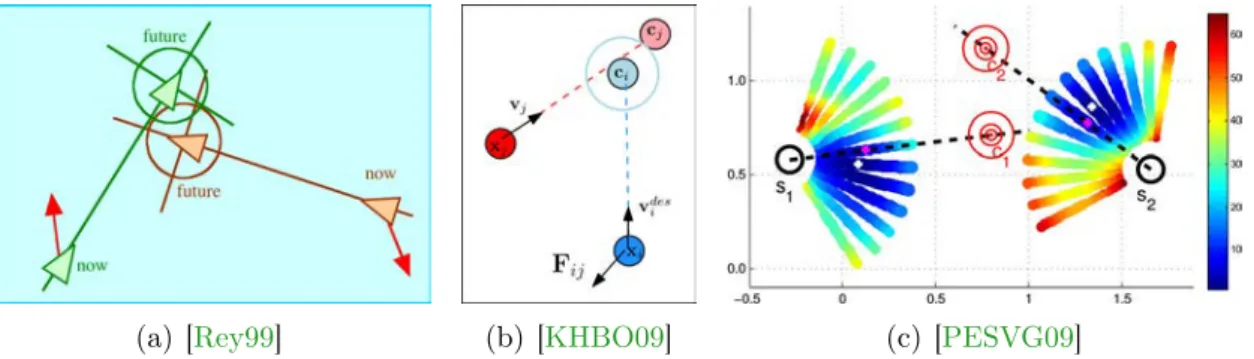
Some algorithms, such as those found in [Rey99] (an extension to the Boids algorithm), [KHBO09] or [PESVG09], predict where a collision between two agents will take place and steer agents away from it, through various repulsive forces (Figure 2.3). Lamarche and Donikian similarly compute future collisions, but then discretize them and identify if those are rear, front, back, or static collisions, with a velocity-adaptation module defined for each type [LD04].

(a) [POO+_{09] (b) [vdBLM08] (c) [Rey99] (d) [HM95]}

Figure 2.2 – Simulation results of two interacting agents [POO+_{09] with second-order}

algorithms (a-c) and a first-order algorithm (d), as compared to ground-truth data. Real trajectories are in red and simulated ones are in blue, the hatched area thus represents the simulation error. Second-order algorithms have a lower error than the first-order one.

(a) [Rey99] (b) [KHBO09] (c) [PESVG09]

Figure 2.3 – Steering away from future collisions. (a) and (b) Repulsion forces are di-rected similarly, Fij is directed by vector −−→cjci in (b). (c) Agents are subjected to repulsive forces originating from each other’s future point of closest approach (e.g. force on agent s1 directed by −−→c2s1).

2.2.2 Collision-Free Velocities

Other algorithms solve collisions in a different way, by searching for a velocity (both the orientation and speed of and agent, usually a two-dimensional vector) leading to a collision-free trajectory. Although the problem is three-dimensional (trajectories are sets of points with a two-dimensional position and a time component), by using agents’ in-stantaneous velocities to linearly extrapolate their future trajectories, the problem can easily be simplified to a two-dimensional one. Consequently, many approaches to colli-sion avoidance have proposed such a simplification, followed by a corresponding solution. For instance, Feurtey defines a disc of points that are reachable with specific velocities in ∆time [Feu00], and chooses agents’ velocity adaptations from this disc based on a cost (cost of colliding, changing direction and changing speed).

Overall, certain velocities lead to a collision while others are collision-free: they are qualified as inadmissible and admissible velocities, respectively. Consequently, Paris et al. [PPD07] divide the space in front of an agent into sections, corresponding to differ-ent oridiffer-entations of said agdiffer-ent (differdiffer-ent colors in Figure 2.4(a)). Then for each section, they determine the speeds that lead to a collision-free motion (in blue in Figure 2.4(b)).

2. AUTONOMOUS AGENT-BASED ALGORITHMS

Finally, the agent chooses among these sections and speeds (combined they form the admissible velocities) those which minimize the velocity adaptation.

(a) Dividing orientations. (b) Dividing speeds.

Figure 2.4 – Agents divide their possible orientation changes (left) and corresponding speed changes (right) during collision avoidance [PPD07]. Purple discs represent the other agent’s positions at diffirent moments in the future. The blue ares on the right represent admissible velocities four one section of possible orientations (each colored area on the left is such a section).

Later algorithms look for admissible velocities in a different way [vdBLM08,GCK+_09,

POO+_{09,GCLM12], and choose instead to reason in the two-dimensional velocity-space}

(see Figure 2.5), where admissible velocities can be quickly found amongst linear con-straints.

(a) [vdBLM08] (b) [POO+_09]

Figure 2.5 – Algorithms reasoning in velocity-space. Left: the main agent (dark gray) is looking for collision-free velocities (white areas) in velocity-space. Light gray areas rep-resent inadmissible velocities leading to collisions with other agents. Right: two agents interacting from the perspective of the bottom left one, with the green area representing inadmissible velocities. The goal of that agent is to move its current velocity (in red) out of the green area to make it an admissible velocity.

2.2.3 Other Predictive Approaches

Finally, some other algorithms have also been proposed, using very different approaches but which are also predictive in nature; the remainder of this section details three such examples.

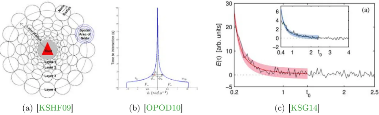
space around an agent is discretized (Figure 2.6(a)) into cells containing information about neighbor agents visiting them in the future; collisions are then solved by choosing an orientation and speed which steer the agent towards the most neighbor-free cells.

Moussaïd and colleagues [MHT11] compute for every direction an agent could follow, a cost based on the time to collision (assuming the agent follows this direction at the current speed, and other agents continue with their current velocity) and the deviation from the destination. They then choose the direction with the lowest cost and adapt the speed of the agent so that the time to collision falls under a certain threshold.

A vision-based algorithm has also been proposed [OPOD10] which simulates agents’ optic flow, and computes for each pixel, the time to closest approach (if there will be a collision, this would then be the time to collision) and the time-derivative of the bearing angle (the angle between the agent’s orientation and a neighbor). Essentially, as the time to interaction decreases (but remains positive) and the derivative of the bearing angle stays close to zero, agents are headed for collision. Thus an agent steers as to keep these two quantities around certain preferred values (see Figure2.6(b)).

In the last example [KSG14], agents are subjected to forces (computed based on linear extrapolations of each agent’s velocity) which have been empirically defined by analyzing recorded ground-truth data, and finding a predictive power law which governs pedestrians’ motions (Figure2.6(c)).

(a) [KSHF09] (b) [OPOD10] (c) [KSG14]

Figure 2.6 – Other predictive algorithms. (a) Illustration of the egocentric discretization of space around an agent, future interactions are stored in these cells. (b) A trajectory is considered collision-free while values of time to closest approach and the time-derivative of the bearing angle stay outside the blue curves. (c) Interaction energy as a function of time to closest approach, extracted from a specific data-set.

2.3 Summary

As a common assumption, these second-order algorithms all linearly extrapolate agents’ future motions from their positions and instantaneous velocities, making it possible to anticipate collisions up to a certain time horizon and improve simulations over first-order algorithms [OMCP12,GvdBL+_12,WGO+_14].

However this remains a linear extrapolation, which in many more challenging sit-uations does not always yield truly satisfactory results, prompting additional work to

3. CENTRALIZED ALGORITHMS

strengthen the quality of simulations. Kim et al [KGL+_{14]. introduced a probabilistic}

component to the algorithm presented in [vdBLM08], while Golas and colleagues [GNL13] added look-ahead to adaptively increase the time horizon in an efficient way for large groups of agents. Finally, this same algorithm has been extended to include agents’ acceleration constraints [vdBSGM11]. All three aproaches have thus extended this algo-rithm to further improve results.

3 Centralized Algorithms

3.1 Cellular Automata

Cellular automata [Sch01, KS08] discretize the simulation space into a grid where each cell can be either free or occupied by one agent (or obstacle). In order to steer agents, these algorithms define rules dictating the probabilities agents have of transitioning into neighbor cells.

The simulation is then carried out as a series of rounds where all agents act in parallel. Each agent first chooses its preferred exit which is the neighbor cell it would attain fol-lowing its preferred velocity during that round (Figure2.7). Afterwards, agents attempt to transition into their preferred exits, while obeying all the rules they are subjected to.

Figure 2.7 – Matrix of preferred transitions for an agent [Sch01].

Figure 2.8 – Conflict between two agents, solved by comparing relative transiton proba-bilities [Sch01].

cupied by another agent and if two agents were to attempt transitioning into the same cell, the one with the highest relative probability is given priority, thus solving extreme congestion cases (Figure 2.8). Rules can also be defined at a larger scale. For instance, it has been observed that two large groups crossing ways lead to the formation of lanes where pedestrians tend to follow the ones in front of them; similarly, pedestrians tend to follow trodden paths rather than unexplored routes. Cellular automata can easily be extended with floor fields to display these phenomena: by increasing agents transition probabilities to recently visited cells, lanes and previously paths will more easily be fol-lowed by subsequent agents. Additionally, these probability increases can be made to decay over time, thus allowing the patterns to change, and preventing the crowds from reducing to a few lanes.

Due to their probabilistic nature, cellular automata allow to evaluate possible out-comes of a given situation. Additionally, thanks to the simplicity of their governing rules, these algorithms scale well. This ability to scale well allows to study the cou-pling/transition from microscopic properties to macroscopic phenomena, such as the for-mation of diagonal patterns between two intersecting traffic flows [CARH13]. For these reasons, they are often used in the field of evacuation dynamics. Due to their discrete nature, these algorithms are not however well suited for computer graphics applications.

3.2 Data-Driven Algorithms

Figure 2.9 – Data-driven algorithms’ usual workflow; from [LCL07].

Data-driven algorithms attempt to learn crowd behaviors from real-world sources such as motion capture or camera footage, hugely benefitting from recent advances in tracking. With large data-sets of real-world pedestrian trajectories available to them, these methods construct data-bases of motions which they then query to synthesize re-alistically behaving crowds. This usual workflow of data-driven algorithms is shown on Figure2.9.

In their work, Lerner at al. [LCL07] aim to determine what influences (and how) pedestrians’ trajectory decisions. Their data-base then consists of pedestrian-interaction examples (see Figure2.10). Each example focuses on one subject pedestrian and captures

3. CENTRALIZED ALGORITHMS

a short moment around a time t. Examples have two components: a portion of the trajectory of the subject, as well as a portion of the trajectories of nearby pedestrians (and other dynamic/static gemoetry such as walls). As seen on Figure 2.10, examples are centered on the subject and all information is recorded in this referential, additionally, each point in this referential has a certain influence value (colored areas in Figure2.10). Each influencing pedestrian (and geometry) is given an influence value corresponding to the highest influence value along their trajctory portion. At run-time, for every agent, the simulation algorithm computes a query and thanks to a similarity function using the influence values, finds the closest example. The trajectory of the subject in the closest example then determines how the queried agent will behave in the simualtion.

(a) (b) (c)

Figure 2.10 – An example as defined in [LCL07]. (a) Configuration of an example, with the subject in the center and nearby influencing pedestrians. Colored areas represent var-ious levels of influence (darker is more influent). (b) The top-right pedestrian’s trajctory portion, the most influential position determines the pedestrian’s influence. (c) All pedes-trians colored according to their influence on the subject.

Other data-driven algorithms follow similar principles. Lee et al. [LCHL07] construct data-bases of state-actions which record information about the subject pedestrian (state: such as speed, neighbors, pivots aka. special objects near which special behaviors take place etc.) and what the pedestrian did. Again, at run-time, this data-base is queried to determine agents’ trajectories.

Ju et al. [JCP+_{10] developed an algorithm which learns crowd formations (as}

distri-butions of the four closest neighbors’ positions) and motions (as trajectory segments) in order to learn different crowd styles. As a result, it is possible to interpolate between different models, thus leading to visually heterogeneous crowds as seen on Figure2.11.

More recently, Charalambous and Chrysanthou [CC14] constructed their data-base in the form of a graph. In this graph, nodes represent the current state of an agent, defined as a series of temporally consecutive visibility patterns (free space in an agent’s field of vision), and edges are actions which allow to transition from state to state. Thanks to this graph structure, run-time queries are easier (the query result is very probably in the agent’s current node) thereby reducing the computational cost as compared to previous algorithms. Additionally, since agents traverse the graph with limited jumping between non-connected nodes (unless they drift too much from the states stored in the current node), their behaviors are more consistent.

Figure 2.11 – Heterogeneous crowd obtained by interpolating between various styles [JCP+_10].

specific styles as well as artist-generated ones can be recorded and used to build the data-bases allowing to synthesize a wide variety of crowds. Additionally, crowds can be randomly initialized (or with some guidance as in [JCP+_{10]) and the agents would}

continue moving according to the learned behaviors seemingly indefinitely without the need for the animator to specify individual goals for each agent. But this lack of explicit goal-management makes agents more difficult to control during run-time. Moreover, the resulting simulations heavily depend on the quality and situation-coverage of the source data. Obviously, situations which are not in the data-base cannot be reproduced and the algorithms can have a hard time when the simulations start straying away from what is learned. Finally, although [CC14] improved run-time performance, these algorithms remain computationally expensive, and are thus better suited for non-interactive appli-cations.

3.3 Tiles and Patches

Tile-based algorithms essentially allow to precompute motions. Using this approach, a virtual environment is assembled from a library of tiles which contain velocity infor-mation, or flows. During simulation, pedestrians are modeled as particles which are advected along these flows, resulting in simulations with a low computational cost. The first technical question then revolves around the construction of these tiles. For instance, Chenney proposes a method [Che04] to create divergence-free tiles, respecting bound-ary conditions imposed by the environment (Figure2.12(a)), while Courty and Corpetti propose to learn the flows from video data [CC07](Figure2.12(b)).

Since all particles (simulated pedestrians) are advected following the same flow fields, these algorithms forgo local collision-avoidance mechanisms. In theory, if particles are initialized as non-intersecting, and allow a certain buffer distance between themselves accounting for the possible compression resulting from the flow fields, collisions should be avoided. In practice however, especially at higher densities collisions do occur. Ad-ditionally, the particles have no individual goals and it is hard to simulate intersecting flows (unless explicitly stacking tiles on top of each other, applicable to specific particles,

3. CENTRALIZED ALGORITHMS

(a) [Che04] (b) [CC07]

Figure 2.12 – (a) Virtual pedestrians walking on tiled streets in a city. (b) Overview of a data-driven tile-based crowd simulation algorithm.

as stated in the future work for these algorithms).

Consequently, Patil and colleagues propose to use a unified solution [PvdBC+_11]

combining a global planner, flow tiles and a local collision-avoidance algorithm. As a result, each agent can select a route along the flow fields (where two opposing flows can intersect) and follow the flow fields, with collisions being solved by the local collision-avoidance algorithm.

While tile-based algorithms create “shared tracks” which advect simulated pedestri-ans, patch-based algorithms take this principle further by creating a track per pedestrian and later assembling them. Thus, Kim et al. build motion patches capturing actors’ in-teractions (hand-shaking, carrying objects etc.), segment them and assemble them dur-ing simulation to create crowds of interactdur-ing characters [KHHL12]. While these whole-body motion patches allow to create crowds of interacting characters, the assembly of patches remains computationally expensive, especially if one wants to keep extending the synthesized scenes. Yersin and colleagues solve this problem [YMPT09] by defining patches which contain periodic character trajectories. By building a library of patches which have matching periodicity and boundary conditions, they are able to effortlessly and endlessly combine patches in all directions, while guaranteeing that the simulation will continue playing forever thanks to its periodicity (Figure2.13).

The main advantage of tile- and patch-based algorithms is their ability to populate virtual areas with large crowds obeying easily controllable pedestrian flows, all at a lesser computational cost during simulation. This property comes at a price however, which is the static nature of the resulting simulations. As all simulated pedestrians are “on tracks” and have no individual navigation (except in the work found in [PvdBC+_{11] where the}

cost increases due to the local collision-avoidance algorithm), the synthesized crowds are non-interactable. Furthermore in the case of tile-based algorithms (and the method from [KHHL12]) on the one hand, edits made to the environment require a re-computation of the tiling, at least to solve any boundary conditions, divergence or singularities that may arise. For the algorithm from [YMPT09] on the other hand, while patches can easily be changed by picking other patches with matching boundary conditions, the efficient (pre-)computation of these patches remains difficult.

(a) (b)

Figure 2.13 – Crowd patches algorithm [YMPT09]. (a) Example of two patches (one period of animation) that can be assembled thanks to matching boundary conditions. (b) Scene assembled from Crowd Patches.

3.4 Macroscopic Algorithms

Crowd simulation algorithms based on fluid-dynamics aim to control very large crowds at the global - or macroscopic - level. Treating the crowd as a flowing continuum, these methods rely on continuous equations, defining flows that the agents (modeled as parti-cles) then follow.

In an extension to the work found in [Hug03], Treuille et al. [TCP06] simulate large, moderately dense crowds of particle-like agents. This method works by combining several fields (discretized into grids), such as goals, speed, density etc. and using the resulting potential field to move agents (see overview Figure 2.14). Inter-agent interactions are solved thanks to the density field: when the density increases it dominates the field equations, thereby pushing agents away from each other (note that this is only ensured down to the level of the grid, meaning that two agents in the same cell can intersect).

Figure 2.14 – Overview of the method from [TCP06].

To improve the agents’ local behavior, Narain et al. [NGCL09] introduced a hybrid method combining fluid-dynamics and a local collision-avoidance method. For each

3. CENTRALIZED ALGORITHMS

agent, a global planner determines the desired velocity (direction and speed), this ve-locity is then tranformed along the agent’s position into flow information contained in a grid. Compressibility constraints are then applied to this flow, so that the crowd is not compressed beyond a threshold. Finally, the corrected flow information is transferred in the form of updated velocities to the agents where pair-wise interactions are solved by the local collision-avoidance algorithm. Figure2.15shows an overview of this algorithm (left) as well as a resulting crowd (right).

These simulators result from a “top-down” process: fluid dynamics-like equations are used to move aprticles, thus defining the local behavior. Some work has also been done from the opposite perspective, as a “bottom-up” process where macroscopic laws are derived from microscopic algorithms (e.g. [BMP11, DARM+_{13, DARPT13] repectively}

derive macroscopic models from (1) cellular automata, and algorithms from (2) [MHT11] and (3) [OPOD10]). This type of derivation can then be used to analyze various aspetcs of crowd motion, such as the formation of clusters of agents for instance.

(a) (b)

Figure 2.15 – Algorithm from [NGCL09]. (a) Workflow overview. (b) Resulting crowd.

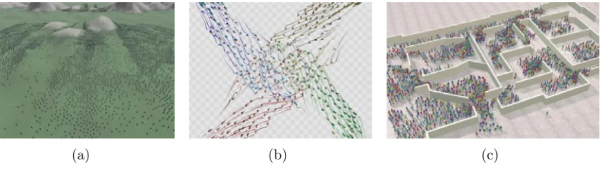
As they steer crowds as a whole and with simplifying assumptions such as shared goals, these macroscopic crowd simulation algorithms scale very well (Figures 2.15(b)

and 2.16(a)) into the tens of thousands of agents at interactive frame-rates. Addition-ally, the resulting simulations seem realistic at the global level and allow the emergence of patterns (e.g. formation of a vortex for four groups crossing ways, Figure 2.16(b)). They also allow controlling a crowd’s density and discover related phenomena such as bottlenecks (Figure2.16(c)). However, these algorithms rely almost exclusively on ter-rain/environment cues to determine the motion of the agents. Additionally, agents are mostly modeled as particles carried by the flow. As a result, agents can have erratic trajectories (going forward/backward and sideways, equally), complex interactions be-tween individual agents are lacking at the local (or microscopic) level, and individual trajectories have little impact on the crowd.

(a) (b) (c)

Figure 2.16 – Crowds generated with macroscpic crowd simulation algorithms. (a) A large army chasing another one. (b) A vortex forms as four groups cross ways. (c) Office evacuation simulation.

4 Conclusion

The first conclusion is that the pool of available algorithms is very large, and the al-gorithms themselves can vary significantly. Each category of alal-gorithms results from a certain need: macroscopic algorithms allow to simulate large crowds observable from a distance/as a whole, tiles and patches allow to easily direct agents with low performance impacts, data-driven algorithms allow to populate areas by “copy-pasting” crowds, cel-lular automata allow to simulate individual agents for statistical purposes, while agent-based algorithms are used for their versatility and general ease of use.

Overall, among all these types of simulation algorithms, each with their strengths and preferred application domains, agent-based algorithms remain the most popular, thanks to their ease of implementation and use but also their flexibility, being intuitively extendable with additional interaction rules and scripting. Agent-based algorithms also yield interactive crowds with consistent levels of realism at all scales: local interaction rules allow to convincingly simulate local behaviors while the resulting crowds display emergent global phenomena observable in real life.

However, despite all the available agent-based algorithms and successive improve-ments, some artifacts still persist in certain scenarios, such as: slowdowns and visu-ally erroneous agent agglutinations, unnatural oscillation motions, or exaggerated/last-minute/false-positive avoidance manoeuvres. Furthermore, one can observe that there are many different simulation algorithms, and that each simulator has its own strengths and weaknesses. To quantify these differences and be able to further develop and improve on existing work, one needs a robust evaluation process. The next chapter (Chapter3) deals with this topic: after a review of previous work on evaluation in Section2, we pro-pose a general evaluation framework, which served as the first step in the work presented in this document.

3

Craal: Parameter Estimation and

Comparative Evaluation of Crowd

Simulations

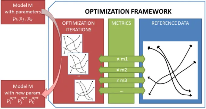
Figure 3.1 – Parameter Optimization Applied to Crowd Data (a) motion capture session for recording reference trajectories for six human agents (b) reference data plot (circles are initial positions) (c) paths taken by simulated agents with default parameters (d) paths taken by simulated agents with optimized parameters. The stock parameters of a simulation model often do not match closely with actual paths humans take in the same situation. Using our parameter optimization technique, the resulting simulation can be made to better match the human trajectories.

Contents

1 Introduction

Creating simulation models of crowds has recently received considerable attention in computer animation, pedestrian dynamics, and virtual reality. As already mentioned in the previous chapter (Chapter2), many approaches have been investigated that suggest different techniques to simulate crowds, and a variety of simulation algorithms are known in the literature. These include multi-agent simulation algorithms that are widely used in computer games, virtual reality, animation, and pedestrian dynamics.

A key research issue in this area is to perform a formal or rigorous evaluation of these algorithms. One widely used criterion is to perform comparative evaluation of simulation algorithms against some real-world reference datasets. However, a major challenge is to estimate the best set of parameters for a given algorithm that would result in the optimal

matchwith the reference data.

The issue of optimal parameter selection is critical, because most of existing crowd simulation algorithms depend on various parameters and the resulting trajectories or behaviors can vary noticeably based on the choices of parameters. There is no standard way to make comparative evaluation of simulation algorithms. At the same time, data capture of real-world human crowd motion is becoming increasingly ubiquitous. Such datasets can in fact help in describing and analyzing specific crowd phenomena, as well as in calibrating and evaluating crowd simulation models. Given the increase in the number of crowd simulation algorithms and real-world datasets, we need rigorous and automatic techniques to evaluate them.

In this work, we present a novel framework that can be used to evaluate different crowd simulation algorithms against reference datasets. In this context, we address the problem of computing optimal parameters for a crowd simulation algorithm and present a general scheme that is applicable to a broad class of algorithms and reference datasets. We formulate the evaluation of a simulation algorithm as an optimization problem. First, we find a set of parameters that enables the best match between each simulation algo-rithm and the reference data. Second, we compare the objective function scores (i.e., distance to reference data) for the given set of algorithms. Our framework is general and capable of supporting a wide range of comparison metrics and simulation techniques.

We illustrate the benefits of our evaluation framework over several existing multi-agent crowd simulation algorithms. Moreover, we consider heterogenous types of refer-ence datasets: recorded individual trajectories, macroscopic quantities, or even anima-tion sketches. We gather a set of relevant metrics to compare simulated crowds with reference data. We highlight the benefits of parameter estimation by demonstrating its application to example-based simulation and behavior modeling with cultural variation. Our framework is available as an open-source package and can be used by others to evaluate different simulation algorithms and metrics. We demonstrate its performance on many widely-used multi-agent simulations and consider different scenarios with a varying number of agents. In our benchmarks, we observe that velocity-based crowd simulation algorithms (e.g. RVO2, [POO+_{09], etc...) result in lower errors as compared}

to techniques based on Boids or social forces.

2. RELATED WORK

on related work in parameter calibration and crowd simulation algorithm evaluation, as a complement to the related work on crowd simulation algorithms from Chapter 2. Section3 describes our parameter estimation framework and its key components: algo-rithms, metrics, reference data, and optimization techniques. A wide range of concrete examples and applications are presented in section4 to demonstrate the benefits of our solution. Finally, we conclude in Section5.

2 Related Work

The necessity of evaluating crowd simulation algorithms arises both in the case of a prospective user when choosing an appropriate simulator, and in the case of researchers and developers when justifying the development of a new one.

The main observation from related work in this aspect is that evaluation is frag-mented across many works and that, while some efforts have been made, no standardized benchmarks are defined and widely accepted in the field of crowd simulation. The reason for this lack of standardized testing is the variety of applications for crowd simulators, leading to the emergence of a wide range of works focusing on very different aspects: by necessity the amount of test cases needs to be large and not all test cases always apply. Section2.1summarizes existing evaluation approaches.

In addition to the lack of a standardized evaluation scheme, one can observe the lack of a standardized evaluation protocol. Mainly, the issue of the simulators’ parameters is rarely taken into account. Thus, resulting comparisons between algorithms can in theory be contested, as “some parameter tweaking” might considerably change the simulations and consequently the comparison results. Related work on the issue of parameters is presented in Section2.2

2.1 Evaluation

In this section we present related work on evaluation, first dealing with the fragmented approaches to this issue and then moving onto attempts at defining standardized testing schemes or benchmarks.

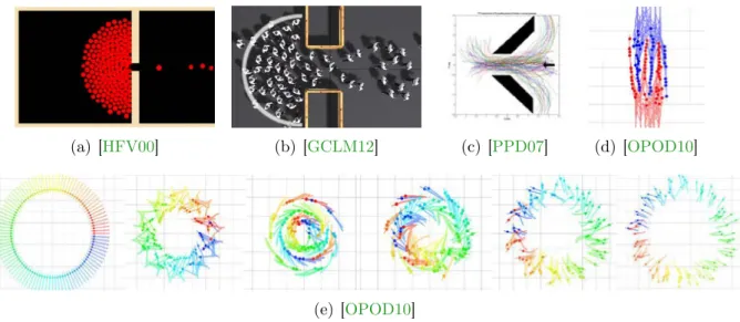
The most direct form of evaluation is the qualitative observation of the simulated crowds. Thus, a number of scenarios are typically chosen to display the ability of a sim-ulator to reproduce known emergent crowd behaviors (Figure3.2). Prominent examples of such behaviors include the circular aggregation of pedestrians around a door/passage, a flow of pedestrians passing throught such passages, and the formation of lanes between two or more flows of pedestrians [HM95,HFV00,PPD07, OPOD10,GCLM12]. In con-trast to these scenarios, which reproduce situations that are readily observable in the real world, other (more artificial) scenarios have subsequently been designed to test how agents interact. In particular, one can force simulated pedestrians to deal with increasing numbers of neighbors by arranging them into a circle and then setting their destinations as the antipodal positions on this circle, effectively maximizing the number of exected interactions. This specific situation, while rarely observed in the real world (and thus lacking ground-truth observations), allows to look for collisions between pedestrians in progressively changing density conditions [vdBLM08,GCK+_09,OPOD10].

(a) [HFV00] (b) [GCLM12] (c) [PPD07] (d) [OPOD10]

(e) [OPOD10]

Figure 3.2 – Examples of test scenarios. (a)-(b) Examples where pedestrians are known to agglutinate in a circular way around a door/passage. (c) Pedestrians traversing a funnel-shaped passage. (d) Lanes forming between two opposing flows of pedestrians. (e) Circle situation where pedestrians attempt to reach the antipodal positions.

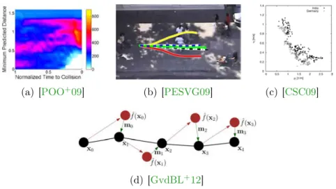
In addition to these typical scenarios, some works have also proposed quantitative evaluations by comparing simulated pedestrians’ trajectories to ones recorded on hu-mans [PPD07, POO+_{09,PESVG09] (Figures3.3(a)and3.3(b)). In these cases, metrics}

included differences between simulated and recorded pedestrians and the minimum pre-dicted distance (distance between two interacting pedestrians when they will be closest to each-other). Guy and colleagues further developed a more complex entropy metric which compares decisions taken by simulated and recorded pedestrians at each step of their trajectories, resulting in a statistical similarity measure between ground-truth and simulation (Figure3.3(d)). Finally, the fundamental diagram (speed of agents in a flow as a function of their surrounding density) can be used (from the field of pedestrian dynamics and evacuation) to evaluate simulated crowds (Figure3.3(c)).

Finally, Singh and colleagues introduced a framework [SKFR09] as an attempt to standardize the evaluation of crowd simulation algorithms. This framework contains a collection of situations destined to cover the range of possible, expected simulation situations (with the question of coverage being explored more in [KWS+_{11]). It also}

contains a collection of metrics measuring for instance the time an agent takes to reach its goal, the energy that has been spent in doing so etc. Similarly, Lerner and colleagues [LCSCO09, LCSCO10] propose a system where a data-base is constructed from trajec-tories extracted from video clips and a set of metrics is used to rate simulated crowds.

2.2 Parameters

When using crowd simulation algorithms, one must keep in mind the algorithms’ pa-rameters, which can range from common ones, such as agent radius or time horizon (if the algorithm is predictive), to algorithm-specific ones such as force magnitude (Social-Forces [HM95] algorithm and similar), various thresholds (e.g. for the time derivative of

2. RELATED WORK

(a) [POO+_{09] (b) [PESVG09] (c) [CSC09]}

(d) [GvdBL+_12]

Figure 3.3 – Examples of ground-truth comparisons. (a) Metric: minimum predicted distance. (b) Comparison of real and simulated trajectories. (c) Fundamental diagram (in this case, difference between German and Indian people for single-line following). (d) The entropy metric compares possibly erroneous simulation decisions (red) to recorded positions (black) at every step.

the bearing angle in the case of the vision-based algorithm [OPOD10]) etc. These pa-rameters are very important as they can have a large impact on the resulting crowds, for instance the wrong value for the force magnitude in the Social-Forces algorithm could lead to agents either colliding (too low value) or walking too far apart/being unstable (too high value). Consequently, this issue greatly influences the evaluation of simulation algorithms, as it is natural to select values for simulators’ parameters that would lead to the best possible results.

The most direct way of setting parameter values is via manual tweaking: the user repeatedly uses the simulation algorithm on various scenarios and gradually settles on values which lead to mostly satisfactory results (either by plotting results or by rule of thumb) [OPOD10]. Paris and colleagues [PPD07] manually set parameter values by checking their results on ground-truth data of two recorded interacting human pedes-trians. Karamouzas and colleagues [KHBO09] plotted results of their algorithm on the various scenarios from the framework presented in [SKFR09] and set their values accord-ingly.

However, this process of manual tweaking is very tedious and some works have au-tomated this process. Pellegrini and colleagues [PESVG09] (seeking to apply their algo-rithm to tracking of humans from video) “train” their algoalgo-rithm on recorded trajectories using gradient descent and a genetic algorithm. Pettre and colleagues [POO+_{09] set their}

parameter values using Maximum Likelihood Estimation based on recorded trajectories of two interacting humans.

More recently, Karamouzas and colleagues [KSG14] derived their algorithm from the power law they had found from collections of real-world data.