The Projective Vision Toolkit

READ THESE TERMS AND CONDITIONS CAREFULLY BEFORE USING THIS WEBSITE. https://nrc-publications.canada.ca/eng/copyright

Vous avez des questions? Nous pouvons vous aider. Pour communiquer directement avec un auteur, consultez la

première page de la revue dans laquelle son article a été publié afin de trouver ses coordonnées. Si vous n’arrivez pas à les repérer, communiquez avec nous à [email protected].

Questions? Contact the NRC Publications Archive team at

[email protected]. If you wish to email the authors directly, please see the first page of the publication for their contact information.

NRC Publications Archive

Archives des publications du CNRC

This publication could be one of several versions: author’s original, accepted manuscript or the publisher’s version. / La version de cette publication peut être l’une des suivantes : la version prépublication de l’auteur, la version acceptée du manuscrit ou la version de l’éditeur.

Access and use of this website and the material on it are subject to the Terms and Conditions set forth at

The Projective Vision Toolkit

Whitehead, A.; Roth, Gerhard

https://publications-cnrc.canada.ca/fra/droits

L’accès à ce site Web et l’utilisation de son contenu sont assujettis aux conditions présentées dans le site LISEZ CES CONDITIONS ATTENTIVEMENT AVANT D’UTILISER CE SITE WEB.

NRC Publications Record / Notice d'Archives des publications de CNRC:

https://nrc-publications.canada.ca/eng/view/object/?id=e9f9cdc8-b54b-4486-9193-ff4ebd3deea0 https://publications-cnrc.canada.ca/fra/voir/objet/?id=e9f9cdc8-b54b-4486-9193-ff4ebd3deea0

National Research Council Canada Institute for Information Technology Conseil national de recherches Canada Institut de technologie de l'information

The Projective Vision Toolkit *

Whitehead, A., Roth, G.

May 2000

* published in the Proceedings, Modelling and Simulation. pp. 204-209, Pittsburgh, Pennsylvania, USA. May 2000. NRC 45874.

Copyright 2000 by

National Research Council of Canada

Permission is granted to quote short excerpts and to reproduce figures and tables from this report, provided that the source of such material is fully acknowledged.

The Projective Vision Toolkit

School of Computer Science Carleton University, Ottawa, Canada

[email protected]

GERHARD ROTH

Visual Information Technology Group National Research Council of Canada

[email protected]

Abstract:

Keywords:Projective Vision, Model Building, Computer Vision

1

Introduction

Uncalibrated computer vision is a topic that has gathered much interest in that last decade [1,2], with a lot of work being done in the last four years. The goal is to produce information about a scene without the aid of calibrated sensors, ultimately to produce a valid 3D model. There have been several systems implemented [3,4,5] that claim to automatically produce these models from an uncalibrated image sequence, yet none have been made publicly available.

We have identified the following basic steps in building a geometric model of a scene from an image sequence: 1 Corner Finding

2 Corresponding Corner Matching 3 Localized Filtering of Matches 4 Computing the Fundamental Matrix 5 Finding Triple Correspondences 6 Computing the Tensor

7 Auto Calibration

8 Building a Metric Model (Valid up to a scale factor) Currently the projective vision toolkit (PVT) allows us to perform steps 1 through 6. We have modularized the tools so that any step of the process can be easily replaced with experimental or more capable software. Although we have not completed the entire process, there is still a lot we can currently do with the PVT. Some applications are covered in a later section titled Current Uses.

Rather than only implementing known existing algorithms, we have also made additions and improvements over existing implementations. The primary benefit that PVT offers is having an entire collection of tools available that work together. However, beyond being just a compellation of necessary tools and known algorithms, our software also has the following features:

• Handles a variety of common file formats (JPG, BMP, GIF, PNG, PPM, PGM)

• Robust corner detection

• Handles larger baselines in the correspondence matcher

• Uses localized filtering to prune incorrect correspondences

• Computes projective and affine fundamental matrices as well as planar warps

• Automatic computation of triple correspondences • It is the only publicly available software that computes

the trilinear tensor

These features represent the beginning of our commitment to creating an invaluable tool for projective vision research. In order to understand the benefits of the toolkit completely, a basic background in projective vision and multi-view geometry is necessary. We continue with this background information in the next section. Readers who already have such a background are referred to section 3. A more complete tutorial can be found at:

http://www.scs.carleton.ca/~awhitehe/PVT/tutorial/

2

Projective Paradigm

To explain the basic ideas behind the projective paradigm, we must first define some notation. We work in homogeneous coordinates, which are defined as an augmented vector created by adding one as the last element. Any projection of a point (in the Euclidean coordinate system) M = [X, Y, Z,1]Tto the image plane m = [x,y,1]Tcan be described using simple linear algebra.

sm = PM

Where s is an arbitrary scalar, P is a 3 by 4 projection matrix, and m = [x, y, 1]Tis the projection of this 3D point onto the 2D camera plane.

If the camera is calibrated, then the calibration matrix C, containing the internal parameters of this camera (focal length, pixel dimensions, etc.) is known. Having this information we can generate the actual 2D image coordinates using this calibration matrix C. Using raw pixel co-ordinates, as opposed to actual 2D coordinates means that we are dealing with an uncalibrated camera system.

Consider the space point, M = [X, Y, Z, 1]T, and its image in two different camera locations;

m1 = [x1, y1, 1]Tand m2 = [x2, y2, 1]T. Then the

well-known epipolar constraint is: m1TEm2= 0

where

E= t

×

where t is the translational motion between the 3D camera positions, and R is the rotation matrix. The essential matrix can be computed from a set of correspondences between two different camera positions [12]. This computational process is considered to be very error prone, but in fact a simple pre-processing data normalization step improves the accuracy and produces a reasonable result [13].

The matrix E encodes the epipolar geometry between the two camera positions. If the calibration matrix C is not known, then the uncalibrated version of the essential matrix is the fundamental matrix F and the epipolar constraint still holds.

m1TFm2= 0

The fundamental matrix can also be characterized in terms of the essential matrix and the camera calibration matrices

F= C1-TEC2-1

This makes it clear that the fundamental matrix contains the information about the calibration matrices and the camera motion.

The fundamental matrix can be computed directly from a set of correspondences by a modified version of the algorithm used to compute the essential matrix. A side effect of computing the essential matrix is the 3D location of the corresponding points. This is also true with the fundamental matrix, but these 3D coordinates are found in a projective space. The camera position is also found when computing F, but again, only in a projective space. There are fewer invariants in a projective space than a Euclidean space, but there are still many useful invariants such as co-linearity and co-planarity. Having camera calibration simply enables us to easily move from a projective space into a Euclidean space. We are not,

however, limited to being in the projective space. We can still easily move to a metric space which only differs from the Euclidean space by a scale factor.

While the fundamental matrix relates the geometry of two views, there is a similar but more elegant concept for three views called the trilinear tensor. Assume that we see the point M = [X, Y, Z, 1]Tin three camera views, and that 2D coordinates of its projections are m1= [x1, y1; 1]T, m2=

[x2, y2, 1]T, and m3= [x3, y3, 1]T In addition, with a slight

abuse of notation, we define mias the i'th element of m1.

It has been shown that there is a 27 element quantity called the trifocal tensor ℑℑℑℑ relating the pixel coordinates of the projection of this 3D point in the three images [1]. Individual elements of ℑℑℑℑ are labeled ℑℑℑℑijk, where the subscripts vary in the range of 1 to 3. If the three 2D co-ordinates (m1, m2, and m3) truly correspond to the same 3D

point, then the following four trilinear constraints hold m3ℑℑℑℑi13mi- m3m2'ℑℑℑℑi33mi- m2ℑℑℑℑi31mi- ℑℑℑℑi11mi= 0

m3ℑℑℑℑi13mi- m3m2ℑℑℑℑi33mi- m2ℑℑℑℑi32mi- ℑℑℑℑi12mi= 0

m3ℑℑℑℑi23mi- m3m2ℑℑℑℑi33mi- m2ℑℑℑℑi31mi- ℑℑℑℑi21mi= 0

m3ℑℑℑℑi23mi- m3m2'ℑℑℑℑi33mi- m2ℑℑℑℑi32mi- ℑℑℑℑi22mi= 0

In each of these four equations i ranges from 1 to 3, so that each element of m is referenced. The trilinear tensor was previously known only in the context of Euclidean line correspondence [14], and the generalization to projective space is recent [15, 1]. The estimate of the tensor is more numerically stable than the fundamental matrix, since it relates quantities over three views, and not two. Computing the tensor from its correspondences is equivalent to computing a projective reconstruction of the camera position and of the corresponding points in 3D projective space. One very useful characteristic of the tensor is image transfer (also called image reprojection). Given any two of m1, m2, and m3, and the tensor ℑℑℑℑ that

describes the geometry between the three images, one can compute where the third point must be.

The fundamental matrix and trilinear tensor can be calculated directly from pixel co-ordinates, and have many important and useful characteristics. We believe that there are four reasons for the recent rapid advances in the projective framework.

1. Basic theoretical work defining the fundamental matrix, trilinear tensor and their characteristics. 2. Simple and reliable linear algorithms for

computing these quantities from a set of 2D image correspondences.

3. Robust random sampling algorithms for filtering noisy and inaccurate correspondences.

4. A suite of algorithms for doing auto-calibration using only the projective camera positions. This combination of advances has made it possible, theoretically, to create a 3D model using VRML of a scene from an image sequence.

3

Description of the Toolkit

We now describe the details of the process that takes an image sequence and computes various projective vision information such as correspondences, fundamental matrices and tensors. In doing so, we highlight the changes and additions that we have made over what are described in the literature.

3.1 Corner Finding

The first step in the process is to find a set of corners or interest points in each image. These are the points where there is a significant change in image gradient in both the x and y directions. We use the public domain SUSAN operator for this function [16]. Rather than setting a corner threshold, we supply an option to return a fixed number of corners. This tends to stabilize the results when the images have different contrast and brightness because the proper threshold is selected automatically. We find that having around 800 corners returned from this tool provides ideal input for the subsequent steps. In the future we plan to make the required number of corners a function of the average image gradient.

3.2 Corner Matching

The next step is to match corners between adjacent images. A local window around each corner is correlated against all other corner windows in the adjacent image that are within a certain working window. The size of the working window represents an upper bound on the maximum disparity between adjacent images. Any corner pair between two adjacent images that pass a minimum correlation threshold and falls within the working window, is a potential match. All potential matches must pass a symmetry test which is define as:

Two corners p and q pass the symmetry test if and only if: • The highest correlation score for p is the corner q • The highest correlation score for q is the corner p The symmetry test reduces the number of possible matches significantly and forces the remaining matches to be one-to-one, but there may be no matches found for a given corner. The total number of possible matches between images is therefore less than or equal to the total number of corner points. Typically, there are only 200 to 500 acceptable matches between 800 pairs of corners. Without the symmetry test constraint there are far more matches; but these matches are much less reliable.

We have improved the capability for handling wider baseline images. We set this upper bound for the working window to be around 1/3 to 1/2 of the image dimensions. We found that it is sometimes useful to relax the symmetry test and to accept the n best matches (usually in the order of 4). Even in this case we still require that the

results be symmetric, that is that each of these matches actually be one of the n best in a symmetric fashion. 3.3 Localized Filtering of Corner Matches

The next step is to perform some type of local filter on these matches. The idea is that just by looking at the local consistency of a match relative to its neighbors it is possible to prune many false matches. This is not always done in the literature, but is sensible, since the computational cost of using a local filter is low. One possible approach used to prune matches is to use relaxation [11]. We use a simpler relaxation-like process to prune false matches, one based on the concept of disparity gradient.

Corner points that are close together in the left image should have similar disparities, and the disparity gradient is a measure of this similarity. Thus, the smaller the disparity gradient, the more the two correspondences are in agreement and vice-versa. We have globalized the comparison so that we compute the disparity gradient of each corner match with respect to every other corner match. The sum of all these disparity gradients is a measure of how much this particular correspondence agrees with its neighbors. We iteratively remove matches until they all satisfy the condition that the match with maximum disparity gradient sum is within a small factor (usually 2) of the match with minimum disparity gradient sum. Using this simple disparity gradient heuristic we are able to remove significant numbers of bad corner matches at a very low computational cost.

3.4 Computing the Fundamental Matrix

The next step is to use these filtered matches to compute the fundamental matrix. This process must be robust, since it can not be assumed that all of the correspondences are correct, even after filtering! Robustness is achieved by using concepts from the field of robust statistics, in particular, random sampling. Random sampling is a "generate and test process" in which a minimal set of correspondences required to compute a unique fundamental matrix, are randomly chosen [6, 8, 9, 17, 7, 11]. A fundamental matrix is then computed from this minimal set. The set of all corners that satisfy this fundamental matrix is called the support set. The random sampling process returns the fundamental matrix with the largest support set.

While this fundamental matrix is correct, it is not necessarily the case that every correspondence that supports the fundamental matrix is valid. This can occur, for example, with a checkerboard pattern when the epipolar lines are aligned with the checkerboard squares. In such a case, the correctly matching corners can not be reliably found using only epipolar lines (i.e. computing only the fundamental matrix). This type of ambiguity can only be dealt with by computing the trilinear tensor.

3.5 Finding Triple Correspondences

We compute the trilinear tensor putative correspondence list (triple correspondences) from the correspondences that form the support set of two adjacent fundamental matrices in the image sequence. Consider three images, i, j and k and their fundamental matrices Fijand Fjk. Each of these

matrices has a set of supporting correspondences, which we call SFij and SFjk. Say a particular correspondence

element of SFijis (xi, yi, xj, yj) and similarly an element of

SFjk is (xj, yj, xk, yk). Now if these two supporting

correspondences overlap, that is if (xj ; yj) in SFij equals

(xj; yj ) in SFjk then the triple created by concatenating

them as a member of CTijk, the set of triple correspondences that a potential members of the support set of the tensor ℑℑℑℑ_{ijk. This process is performed using all} sets of adjacent images in the sequence. With the set of putative triple correspondence, we can now continue by computing the trilinear tensor.

3.6 Computing the Tensor

Here we again employ the random sampling algorithms. We use a randomly selected set of correspondences to compute the tensor with the largest support. The result is the tensor ℑℑℑℑ_ijk, and a set of triples (corresponding corners in the three images) that actually support this tensor, which we call Sℑℑℑℑ_{ijk. As before, we provide more than a} single mechanism for computing the tensor, by offering a variety of methods for use and review.

3.7 Visualizing the Results

Using the toolkit, we have gone from a set of images i, j, k and computed a set of corner points Ci; Cj, and Ck; to a set of matches Mij , and Mjk; to a set of filtered matches DMij , and DMjk; to a pair of fundamental matrices Fij, Fjk and their support sets SFij and SFjk; to a set of computed triple correspondence Cℑijk, to a tensor ℑijk with support Sℑijk. Note that the cardinality of the supporting matches always decreases, but the confidence that each match is correct increases. The entire process begins with many putative matches, and refines these to a few high confidence matches. The final matches that support the tensor (Sℑijk), range in cardinality from 20 to 100, and in practice, have a very high probability of being correct.

After all the computations are complete, we still find ourselves with a large amount of data. The toolkit provides a mechanism to visually display each of the supports sets, along with motion vectors and correspondences. The tool will also allow you to perform epipolar and tensor transfers at runtime.

4

Current Uses

As mentioned previously, the toolkit is ideal for work in uncalibrated computer vision. But this does not preclude its use in the world of calibrated vision. Numerous examples have show that generating correspondences in the projective domain is an easy task when using the toolkit.

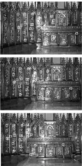
Figure 1:Correspondences automatically found by PVT Should calibration information be available, it can be used to compute the 3D camera positions from these correspondences. Such results have been demonstrated experimentally on a number of examples [18] where the triple correspondences are chained together and used as input to the Photomodeler[10] program. This has produced a Euclidean reconstruction of multiple camera positions while greatly reducing the effort of selecting the correspondences manually.

Not only can the toolkit be used in practical applications, it is also useful as a teaching tools for learning concepts in projective geometry. Having the ability to compare and contrast algorithms, as well as being able to visualize the results, helps to reduce some of the complexities new students often face when learning the essentials of

projective vision. The modularity of the toolkit makes it possible to experiment with new algorithms while maintaining a consistent and reliable interface for the rest of the process.

5

Future Additions

It is our intention to provide all the necessary tools to complete the model building process. To this effect, in future versions we hope that PVT will include:

• Video support with automatic frame extraction • Auto-calibration routine to find at least the focal

length

• Projective Vision Tutorial that uses the toolkit as a teaching aid

• Model building tools to create VRML worlds

6

Conclusions

We have developed a modular system that is capable of using the projective vision paradigm to automatically find correspondence points in an image sequence. It has shown its immediate use in the field of photogrammetry, and as an academic learning tool. We have implemented robust corner detection, handle larger baselines in the correspondence problem, introduced localized filtering, computes projective and affine fundamental matrices as well as planar warps, and automatically compute triple correspondences. As well, to our knowledge this is the only publicly available software that computes the trilinear tensor. We have also provided a mechanism to view the results that the toolkit produces.

We invite you to download the toolkit and try it on your own image sequences. The toolkit is available on a variety of platforms including Windows 95/NT, Linux, SGI, and Solaris. Further documentation, as well as many examples are available at:

http://www.scs.carleton.ca./~awhitehe/PVT

References

[1] A. Shashua, Algebraic functions for recognition, IEEE Transactions on Pattern Analysis and Machine

Intelligence, vol. 17, no. 8, pp. 779-789, 1995.

[2] R. I. Hartley, Self-calibration of stationary cameras, International Journal of Computer Vision, vol. 22, pp. 5-23, February 1997.

[3] R. Koch, M. Pollefeys, and L. VanGool, Multi viewpoint stereo from uncalibrated video sequences, Computer Vision-ECCV'98, pp. 55-71, 1998. [4] M. Pollefeys, R. Koch, M. Vergauwen, and L. VanGool, Automatic generation of 3d models from

photographs, Proceedings Virtual Systems and MultiMedia, 1998.

[5] A. Fitzgibbon and A. Zisserman, Automatic camera recovery for closed or open image sequences, ECCV'98, 5th European Conference on Computer Vision, pp. 311-326, Springer Verlag, June 1998.

[6] Z. Zhang, R. Deriche, O. Faugeras, and Q.-T. Luong, A robust technique for matching two uncalibrated images through the recovery of the unknown epipolar geometry Artificial Intelligence Journal, vol. 78, pp. 87-119, October 1995.

[7] P. Torr and D. Murray, Outlier detection and motion segmentation, Sensor Fusion VI, vol. 2059, pp. 432-443, 1993.

[8] P. J. Rousseeuw, Least median of squares regression, Journal of American Statistical Association, vol. 79, pp. 871-880, Dec. 1984.

[9] R. C. Bolles and M. A. Fischler, A ransac-based approach to model fitting and its application to finding cylinders in range data, Seventh International Joint Conference on Artificial Intelligence, pp. 637-643, 1981. [10] Photomodeler by EOS Systems Inc.

http:/www.photomodeler.com.

[11] G. Xu and Z. Zhang, Epipolar geometry in stereo, motion and object recognition. Kluwer Academic, 1996. [12] H. Longuet-Higgins, A computer algorithm for reconstructing a scene from two projections, Nature, vol. 293, pp. 133-135, 1981.

[13] R. Hartley, In defence of the 8 point algorithm, IEEE Transactions on Pattern Analysis and Machine

Intelligence, vol. 19, 1997.

[14] M. Spetsakis and J. Aloimonos, Structure from motion using line correspondences, International Journal of Computer Vision, vol. 4, pp. 171-183, 1990 1990. [15] R. Hartley, A linear method for reconstruction from lines and points, Proceedings of the International Conference on Computer Vision, pp. 882-887, June 1995. [16] S. Smith and J. Brady, SUSAN - a new approach to low level image processing, International Journal of Computer Vision, pp. 45-78, May 1997.

[17] P. Torr and A. Zisserman, Robust parameterization and computation of the trifocal tensor, Image and Vision Computing, vol. 15, no. 591-605, 1997.

[18] G. Roth and A. Whitehead, Using Projective Vision to Find Camera Positions in an Image Sequence, Vision Interface, May 2000