A fast implementation of a spectral finite elements method on CPU and GPU applied to ultrasound propagation

HAL Id: hal-01761605

https://hal.archives-ouvertes.fr/hal-01761605

Submitted on 25 Nov 2018

HAL is a multi-disciplinary open access

archive for the deposit and dissemination of

sci-entific research documents, whether they are

pub-lished or not. The documents may come from

teaching and research institutions in France or

abroad, or from public or private research centers.

L’archive ouverte pluridisciplinaire HAL, est

destinée au dépôt et à la diffusion de documents

scientifiques de niveau recherche, publiés ou non,

émanant des établissements d’enseignement et de

recherche français ou étrangers, des laboratoires

publics ou privés.

A fast implementation of a spectral finite elements

method on CPU and GPU applied to ultrasound

propagation

Carlos Carrascal-Manzanares, Alexandre Imperiale, Gilles Rougeron, Vincent

Bergeaud, Lionel Lacassagne

To cite this version:

Carlos Carrascal-Manzanares, Alexandre Imperiale, Gilles Rougeron, Vincent Bergeaud, Lionel

La-cassagne. A fast implementation of a spectral finite elements method on CPU and GPU applied to

ultrasound propagation. International Conference on Parallel Computing, ParCo Conferences, Sep

2017, Bologna, Italy. pp.339 - 348, �10.3233/978-1-61499-843-3-339�. �hal-01761605�

A fast implementation of a spectral finite

elements method on CPU and GPU

applied to ultrasound propagation

a_{CEA-LIST, Centre de Saclay, 91191, Gif-sur-Yvette Cedex, France}

b_{Sorbonne Universit´es, UPMC Univ Paris 6, CNRS UMR 7606, LIP6, Paris, France}

Abstract. In this paper we present an optimization of a spectral finite element method implementation. The improvements consisted in the modification of the memory layout of the main algorithmic kernels and in the augmentation of the arith-metic intensity via loop transformations. The code has been deployed on multi-core SIMD machines and GPU. Compared to our starting point, i.e. the original scalar sequential code, we achieved a speed up of ×228 on CPU. We present comparisons with the SPECFEM2D code that prove the good performances of our implementa-tion on similar cases. On GPU, a hybrid soluimplementa-tion is investigated.

Keywords. Spectral Finite Elements, parallelization, vectorization, SIMD, GPU

1. Introduction

In the context of ultrasonic non-destructive testing (NDT) simulation, a new finite ele-ment method based on the spectral finite eleele-ments and the domain decomposition method has been developed in the CIVA software [1]. As the computational cost of such a nu-merical method is expensive, our goal is to reduce the simulation time by an efficient use of the hardware to reach the speed expected by the NDT engineers who are mainly equipped with standard PCs or workstations.

First, we will perform an overview of the spectral finite elements and the domain decomposition method. Secondly, the equation will be split into workable stages to anal-yse the performance and which optimizations can be efficient, like memory layout opti-mizations and loop transformations. Thirdly, an analysis of accuracy, hardware architec-ture, scalability and vectorization on several multi-cores machines will be presented. We will compare our code performance with SPECFEM2D, a well-known software imple-mentation of SFEM. A feasibility study will be also performed on GPU. Lastly, we will conclude and draw some perspectives.

1_{Corresponding Author: Carlos Carrascal-Manzanares, CEA Saclay, Digiteo Labs, P.C. 120, F-91191}

2. Overview of the Numerical Method

The ECHO library simulates ultrasounds controls to detect echoes on cracks. It has to model the propagation of waves inside a component several order bigger. For this, it combines the domain decomposition method and the Spectral Finite Element Method (SFEM) to solve the problem.

The SFEM is a powerful tool for solving the wave equation. It relies on high-order finite element spaces while conserving a fully explicit scheme, thanks to the mass lump-ing technique [2]. For example, applylump-ing an explicit time discretization of order two, which is stable under the so-called Courant-Friedrichs-Lewy condition on the time step, the fully discrete equation obtained reads

M Ð→ Pn+1−2Ð→Pn+Ð→Pn−1 ∆t2 +K Ð→ Pn= MÐ→Fn (1) whereÐ→P is the unknown, n represents the time step, M is the mass matrix, K is the stiffness matrix andÐ→F is the source. In practice, in order to apply the SFEM, the domain needs to be discretized by a mesh composed of hexahedral elements, which are known to be a major challenge for meshing algorithms [3].

This method has been extensively used: to solve transient wave equations [4], elas-todynamic multi-dimensional problems [5] or targeting seismic problems [6][7] using also GPU hardware [8] and distributed computation [9][10].

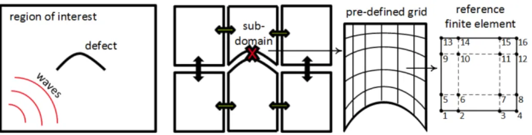
The region of interest, where the cracks are situated, is decomposed into deformed cubes, which are called sub-domains. The cracks are situated as boundaries between two or more domains where the wave propagation is altered or interrupted. Each sub-domain corresponds to a deformed predefined grid. Every element is associated with a reference spectral finite element. In this reference element, high-order lagrangian func-tions are defined using Gauss-Lobatto points [11]. Using an approximation order q leads to q+ 1 symmetrical DoFs per dimension. In order to reduce sub-domains communica-tions we impose one-to-one interfaces and same DoF position within common interfaces. This strategy allows us to solve explicitly interface problems arising from domain de-composition. Hence the computational burden is mostly related to computational steps.

Figure 1. From left to right: a 2D surface with a parametric defect; the same surface divided into six sub-do-mains; a deformed pre-defined grid; a finite reference element and 16 DoFs located by a quadrature rule of order 3.

3. Optimization of the Stiffness Matrix 3.1. Local Stiffness Matrix

Since the mass matrix is diagonal, the main computational effort (75% of the total ex-ecution time) comes from the product of the stiffness matrix with the previously com-puted solution vector. Thanks to the SFEM, the structure of the global stiffness matrix is composed of overlapping local stiffness matrices related to every element in the mesh.

In the context of ultrasound propagation modelling, storing the global stiffness is numerically intractable, due to the huge number of elements in the mesh. Hence, we opt for an unassembled strategy where the product between the local stiffness matrices and the finite element vector corresponding to each element is performed on the fly. The only constraint to the unassembled strategy is that the local products within a sub-domain with two elements sharing DoFs (neighbours) cannot be computed at the same time. For this, we use a colouring strategy that gives a color to each element, knowing that two neighbours cannot have the same colour (that is, 4 colors in 2D, 8 colors in 3D). Then, each group of colours can benefit from parallel computing. The colouring strategy is also explicit and does not add heavy complexity. A similar strategy was followed in [8], with the added complexity of dealing with unstructured meshes. In the following, working on the elements of the same colour is supposed, eliminating all constraints regarding concurrent accesses in the parallelization.

3.2. Stage Decomposition

In this paper, we shall address the case of a two-dimensional acoustic wave equation and a propagation inside an isotropic homogeneous material, but other cases, as three dimensions, elastic wave equation and anisotropic materials, have also been treated. The resulting equation is Eq. (2), where the input U represents the local finite element vector of size(q + 1)2, and the output is the vector with the product. A is the gradient matrix, and AT is its transposition. co(DF) is the cofactor of the linear transformation F and JFthe jacobian of F. These terms are related to the transformation and they are applied

to each local DoF, a vector of two dimensions. ˆcis the wave speed, which is constant because of the homogeneous isotropic nature of the material. From an algorithmic point of view, this equation can be divided in 5 stages in accordance with their main function.

V ® Stage 4 = AT ¯ Stage 3 ⎛ ⎝cˆ co(DF)Tco(DF) ∥JF∥ ⎞ ⎠ ˆx_i ´¹¹¹¹¹¹¹¹¹¹¹¹¹¹¹¹¹¹¹¹¹¹¹¹¹¹¹¹¹¹¹¹¹¹¹¹¹¹¹¹¹¹¹¹¹¹¹¹¹¹¹¹¹¹¹¹¹¹¹¹¹¹¹¹¹¹¹¸¹¹¹¹¹¹¹¹¹¹¹¹¹¹¹¹¹¹¹¹¹¹¹¹¹¹¹¹¹¹¹¹¹¹¹¹¹¹¹¹¹¹¹¹¹¹¹¹¹¹¹¹¹¹¹¹¹¹¹¹¹¹¹¹¹¹¹¶ Stage 2 A ® Stage 1 ⋅ U ® Stage 0 (2)

More specifically, stage 0 finds the degrees of freedom corresponding to a local element on the global vector and then copies them to a local vector. Stage 1 computes the gradient as a product of an invariant matrix by this local vector. Stage 2 consist in two two-dimensional matrix products, adding some scalar products for each DoF. Stage 3 computes the transposed gradient, which are the same calculations as in stage 1. This last one is finally accumulated on the global vector by means of stage 4.

3.3. Memory Layout

In order to select which optimization to apply, we first compute the arithmetic intensity (AI) which is the ratio between computations and memory accesses. A small AI usually leads to memory bound algorithm. The original code has an average AI value of 0.5 for approximation order 2 (further details are shown in Table 1). The main target of the following optimizations is to reduce the amount of memory accesses.

Table 1. Computations and memory accesses for the original code, the memory layout optimizations and the loop transformations in each stage for the approximation order 2.

Computation / IOs Stage 0 Stage 1 Stage 2 Stage 3 Stage 4 Total AI Original 0/18 108/234 198/315 108/225 18/27 432/810 = 0.5 Memory Layout 0/27 108/216 117/45 108/216 27/36 360/540 = 0.7 Loop Transformation 0/9 90/0 162/0 90/0 27/18 369/27 = 13.7

Let us focus on stage 1 and then apply the optimizations to stage 3, as it is mostly the same calculation. The gradient matrix, A, is a regular sparse matrix. Most of the co-efficients are zero, and the non-zero ones follow a regular structure. There is a different matrix A for each dimension. Each (i, j) coefficient shows the relation between the DoF i and the DoF j. Thanks to the finite element of reference, the DoFs elements are sym-metrically situated in each dimension with repeated pattern. Considering second order, the reference element size is 9 DoFs and thus there are only 9 different coefficients. As shown in Figure 2, we decided to store once each coefficient, creating a reorganized copy of the local vector to match the new and smaller matrix product. In this example two 9×9 matrix products are reduced to six 3×3 matrix products.

Figure 2. Schema of stage 1 calculations. One gradient for each dimension is converted into several small matrix-vector products using the same smaller matrix.

As Figure 2 shows, the second vector is reorganized. This new memory layout sim-plifies the code because multiple chained loops with strided accesses become only one loop performing basic small products. We apply the same ideas to stage 3, but using the transposed matrix. Other stages are modified to suit the new layout. Stage 2, being in the middle of this optimizations, benefits largely regarding both memory accesses and computations. New AI values can be found in Table 1. This technique should reduce the number of cache misses.

3.4. Loop Transformation

Loop unwinding and scalarization [12][13] have been applied. It pursues operator fusion and reduces the amount of memory accesses (or increasing the AI). The code is divided in three pieces: memory loads, computations and memory stores. The data is loaded into and stored from scalar variables. The strided accesses are reduced, therefore allowing the compiler to optimize the code freely. Complex codes with multiple reused values can benefit largely, although the resulting code may be longer. After applying this transfor-mation in all stages, the code has an average AI of 13.7 (see Table 1), which means it is computed bound.

4. Benchmark & Analysis

To benchmark our code, we selected a configuration of a two-dimensional mesh of 64 million global DoFs (that is 8,000 for each dimension), with a polynomial approxima-tion order from 2 to 10. The code solving the stiffness matrix product is intended to be used from order 2 to 5, but the range has been extended to gather more information. As the global points are fixed, increasing the elements size results in decreasing the number of total elements. That allows to evaluate the relation between the order and the opti-mizations. It should be highlighted that computing each local element separately leads to compute much more DoFs than 64 million because of repeated DoFs in borders. It should also be noted that the bigger the element is, the smaller the border ratio is, and thus less DoFs are computed.

Table 2. Millions of elements and computed DoFs against approximation order for 64 million points mesh (values are rounded).

Order 2 3 4 5 6 7 8 9 10

Elements (M) 16 7 4 2.5 1.8 1.3 1 0.79 0.064 Computed DoFs (M) 144 114 100 92 87 84 81 79 77

64 million global points on 32-bit floating points leads to a 1.4GB-size problem. The unit of measure selected is cycles per point (cpp), that is total clock cycles (RDTSC instruction) divided per computed DoFs [see Table 2]. All measurements correspond to one time step. The processors used are specified in each case. Turbo-boost and hyper-threading are always disabled. Code is compiled with Intel C++ Compiler 17.0 and high-est optimization flag (O3). The source code is parallelized using a # pragma omp parallel OpenMP directive and vectorized using only # pragma ivdep directives.

4.1. Accuracy Analysis

Single precision floating point values are used, although the original code used double precision values. This change have been decided based upon the relative error when using single precision compared with a double precision result. To do so, the biggest difference between the points of a defined step is compared with the biggest value in that time-step. After 500 time-steps, the relative error is for all approximation orders smaller than 0.01%, and after 5000 time-steps smaller than 0.1%. The error grows linearly with the number of steps and can be limited.

4.2. Impact Analysis

Four machines have been used for benchmarking: Westmere (WSM) 2× 6 cores Intel Xeon Processor X5690 3.46Ghz, Ivy Bridge (IVB) 2×4 cores Intel Xeon Processor E3-1245 v2 3.45GHz, Haswell (HSW) 2×8 cores Intel Xeon Processor E5-2630 v3 2.4GHz and Broadwell (BDW) 2× 10 cores Intel Xeon E5-2640 v4 2.4GHz. The following test is performed with the IVB machine. The optimized code is faster in every case than the older code using a scalar mono-thread execution (Figure 3). The cache misses have been reduced in a 50% and the acceleration factor is on average 3. It seems to use less cpp before approximation order 7 and much more after order 8. By using Intel VTune Am-plifier XE, an increase of instruction cache misses has been measured from insignificant to around 10%. This is related to the increasing size of the code with the order, from 240 lines for approximation order 2 to 1520 lines for approximation order 10. In order to know if the issue can be overcomed varying the processor architecture, this version has been tested with WSM, IVB and HSW. The L1 cache sizes used are 64KB, 16KB and 32KB respectively. As shown in Figure 4, HSW does not meet the problem until the approximation of order 12, using a smaller L1 cache than WSM. HSW must implement a different algorithm to handle the instructions cache misses, but the information about these algorithms is scarce, so it is just a guess. Regarding why WSM performs better than IVB, the L1 cache sizes difference may be the reason. Then using HSW, the acceleration factor is on average 4.5.

Figure 3. Cpp by approximation order+1 comparing a scalar mono-thread execution using a IVB proces-sor.

Figure 4. Performance of the code using WSM, IVB and HSW processors. The abscissa has been extended to observe the deferred effect.

4.3. Scaling and Vectorization Efficiency

For clarity, only the first four approximation orders are kept during this section. Then the acceleration factor is on average 5.3. The machine used is the HSW. Our new code ben-efits of great vectorization and scalability efficiency. The test compares a scalar mono-thread execution against 2 up to 16 scalar OpenMP mono-threads. Before optimizations, the code had an efficiency of around 22%. Now the efficiency goes from 97% using two threads to 90% using sixteen (Figure 5).

Then we evaluated the impact of different SIMD extensions, comprising SSE4.2 and AVX2 instructions without and with FMA. The theoretical speed up factors are 4, 8 and

Figure 5. Scalability of the new code. Figure 6. Vectorization impact of the new code.

16 respectively. Before, the vectorization efficiency with AVX instruction was of 26%. The efficiency now is respectively around 100%, 75% and 35% (Figure 6).

Some NUMA issues in bi-processor configuration have been found when combin-ing OpenMP with SSE4.2 and AVX. As HSW has two processors, the first one is used efficiently but the second one suffers a fall of performance. Using SSE4.2 instructions (Figure 7), the first eight threads have an efficiency of around 95%, but then it falls to 50%. On the other hand, AVX performs around 90%, then decreases to 30%, to increase again to 80%. This roller coaster is closely related to our memory layout. The loop is divided between the threads, which process process elements that can be situated in the same line and be ’reasonably’ contiguous, or through different lines. Depending on the number of threads and the problem size, this can highly affect the NUMA nodes, or not at all. The code has been tested with different NUMA node sizes, and there are always some strong disturbances using the second one.

Figure 7. Scalability of the SSE4.2 code. Figure 8. Scalability of the AVX code.

Finally, the 8-core AVX version using the HSW machine is ×228 faster than the original scalar code.

4.4. Comparative Benchmark with SPECFEM2D

SPECFEM2D [14] is the reference software for seismic wave propagation in two-dimensional acoustic and elastic media. Both codes use spectral finite elements for sim-ulation but at different scales: ECHO is coded for NDT and SPECFEM2D is used in

geodynamics. Until now, only the product of the stiffness matrix has been discussed. For comparison, the capability to solve the entire wave equation (Eq. (1)) has been added, using the same methodology when possible.

The machine used is the BDW. An approximation order of 2 is used, because SPECFEM2D only allows orders 1 and 2. SPECFEM2D uses a square mesh generated with the pre-processing finite element mesh generator Gmsh. The same source and sim-ilar variables has been settled between the two codes. SPECFEM2D has been modified to remove all output and related checks it usually does, to compare only computation time. 2,000 time-steps are used. In this case, both codes use a call to CPU time, so the elapsed time is given in seconds, not cycles. The measured scale is time per element. Both of them have been compiled with the Intel compiler, ICC in our code and IFC for SPECFEM2D. OpenMP and AVX2 vectorization flags have been activated. To be fair, we can not compare multi-threading execution. SPECFEM2D is designed to use distributed architectures via MPI, whereas our code is intended to use OpenMP in single worksta-tions. Our code benefits of great scalability but SPECFEM2D suffer with MPI commu-nication overhead, which is pointless using this kind of architecture. We are therefore comparing mono-thread executions.

Table 3. DoFs, elements and execution time of our code and SPECFEM2D.

DoFs Elements Total seconds Seconds per element SPECFEM2D 130561 32480 1.46 × 10−2 _{4.48 × 10}−7

ECHO 133225 33124 1.76 × 10−3 5.30 × 10−8 Speed up factor ×8.45

As shown in Table 3, our code has a substantial speed up factor. There are multiple reasons. First, SPECFEM2D aims at treating more general geometries than our code and therefore supports unstructured meshes. This more generic data structure may provoke indirect accesses and more complex memory layouts. Secondly, according to the Intel optimization report, few loops have been vectorized, because vector dependence prevents vectorization.

4.5. GPU: a Feasibility Study

Our optimized stiffness algorithm has a high AI and a good parallel efficiency. It should therefore benefit from GPU computational power. Our interest is to target one single GPU, as did Huthwaite [15], but it can be done using several GPUs [9]. The are two main issues regarding the efficient use of GPUs: transfer time and computation time.

The input memory (which is going to be read during stage 0) and the output memory (which is written during stage 4) need to be transferred. The constant coefficients are negligible. Furthermore, these transfers will not fit the GPU global memory in a context of multi-domain problems, where the meshes need dozens of gigabytes [8]. Our strategy is to load (potentially several) domains in order to fill in the GPU memory and compute one temporal iteration before replacing it with a new domain. These memory transfers can be asynchronous, so they can be hidden. Our tests use a NVIDIA GeForce GTX TITAN, 6GB of global memory, Kepler GK110, 0.8GHz, compute ability 3.5 and 2048 single precision cores. This GPU is connected through a PCI Express x16 2.0. The code is written in CUDA and compiled with NVCC. We consider a two-dimensional mesh

of 640 million global DoFs. The problem size is 4.2GB, half input, half output. The bandwidth achieved is 6.29GB/s out of the ideal 6.4GB/s transfer bandwidth given by the tool CUDA Bandwidth Test (that is 749ms). This bandwidth could be higher using a motherboard connection with architecture PCI 3.0, going up to 10.8GB/s.

Regarding the computing time, there are up to 64 warps of 32 threads each and 65536 registers to be distributed equally. Occupancy is fulfilled if all the 64 warps are in use, that is using 2048 threads and having 32 registers for each one. A single thread can not use more than 255 registers. Balancing the warp used against register availability is crucial, because high occupancy is not always better [16].

The GPU version of the code computes one element using one thread. Shared mem-ory is not used because threads does not access same positions. The cudaOccupancy-MaxPotentialBlocks function helps us to calculate the maximal size of one block con-sidering how many registers the kernel uses (it depends on the approximation order, see Table 4). The code presents two main issues. The first one is that a single thread requires a lot of registers and thus the occupancy decreases. The second issue is about memory layout. As each thread load an element, and the elements are not adjacent, the threads cannot load coalesced memory.

Table 4. Values related to the GPU algorithm. Each column from left to right: approximation order+1, registers used in each kernel, block size, active warps in GPU at the same time, its proportion against 64 total warps, GPU execution time and CPU execution time (seconds) using the fastest CPU version (HSW mono-socket using AVX instructions).

Order+1 Registers/thread Threads/block Active warps Occupancy GPU time CPU time

3 71 32x28 28 43.75% 1.57 1.00

4 101 32x16 16 25.00% 1.82 0.81

5 135 32x12 12 18.75% 2.20 0.73

6 181 32x8 8 12.50% 2.98 0.74

The GPU version is slower than our fastest CPU code considering execution time. Our current work is trying to limit the register number to increase the GPU occupancy. We plan to use the maxrregcount flag combined with kernel launch bounds to control the number of registers. By increasing the warps used and the occupancy, the hypothesis is that the performance will be increased.

Even when the GPU is not still fully used, we plan to develop a hybrid computation strategy, following the ideas of Papadrakakis [17]. As all the information regarding the use of different approximation orders is available, we will be able to add an auto-tuning step, as did Dollinger [18]. We expect to predict the execution time launching a small test-case with different approximation orders and sub-domains sizes, and then decide consequently the placement.

5. Conclusion and Perspectives

A fast SFEM implementation has been presented. We have performed memory layout optimizations and code transformations to increase the arithmetic intensity and reduce the cache misses. Further loop optimizations lead to a code automatically vectorized and parallelized which is several order faster than the original code. A comparative bench-mark of execution time has been performed between SPECFEM2D and our code,

show-ing a significant performance improvement. Finally, a feasibility study regardshow-ing the use of GPUs has been conducted.

A particular case of the wave equation has been presented. Our next step will be to apply the work done to a wider range of cases: dimension, materials, transformations. Using these code transformations means having one source file for each approximation order (potentially 2 to 10), which size can be considerable. Combining the different bi-nary parameters leads to 144 files for each hardware. We therefore plan to generate au-tomatically these files from another program.

References

[1] Imp´eriale et al., UT simulation using a fully automated 3D hybrid model: application to planar backwall breaking defects inspection, Quantitative Nondestructive Evaluation Conference (2017).

[2] Cohen et al., Higher-order finite elements with mass-lumping for the 1d wave equation, Finite Elements in Analysis and Design 16 no.3 (1994), 329-336.

[3] Shepherd et al., Hexahedral mesh generation constraints, Engineering with Computers 24 no.3, (2008), 195-213.

[4] Cohen, Higher-Order Numerical Methods for Transient Wave Equations, Springer, 2002.

[5] Casadei et al., A mortar spectral/finite element method for complex 2D and 3D elastodynamic problems, Computer Methods in Applied Mechanics and Engineering 191 no.45 (2002), 5119-5148.

[6] Komatitsch et al., Introduction to the spectral element method for three-dimensional seismic wave prop-agation, Geophysical Journal International 139 no.3 (1999), 806-822.

[7] Komatitsch et al,. The spectral element method: An efficient tool to simulate the seismic response of 2D and 3D geological structures, Bulletin of the Seismological Society of America 88 no.2 (1998), 368-392.

[8] Komatitsch et al., Porting a high-order finite-element earthquake modeling application to NVIDIA graphics cards using CUDA, Journal of Parallel and Distributed Computing 69 no.5 (2009), 451-460. [9] Komatitsch et al., Modeling the propagation of elastic waves using spectral elements on a cluster of 192

GPUs, Comput. Sci. Res. Dev.25, no.1-2 (2010), 75-82.

[10] Komatitsch et al,. High-order finite-element seismic wave propagation modeling with MPI on a large GPU cluster, Journal of Computational Physics 229 no.20 (2010), 7692-7714.

[11] Durufle et al., Influence of Gauss and Gauss-Lobatto quadrature rules on the accuracy of a quadrilateral finite element method in the time domain, Numer. Methods Partial Differential Eq. 25 no.3 (2009), 526-551.

[12] Kennedy et al., Optimizing Compilers for Modern Architectures: A Dependence-based Approach, Mor-gan Kaufmann Publishers Inc. (2002).

[13] Lacassagne et al., High Level Transforms for SIMD and Low-level Computer Vision Algorithms, ACM Workshop on Programming Models for SIMD/Vector Processing (PPoPP) (2014), 49-56.

[14] Tromp et al., Spectral-element and adjoint methods in seismology, Communications in Computational Physics 3 no.1 (2008), 1-32.

[15] Huthwaite, Accelerated finite element elastodynamic simulations using the GPU, Journal of Computa-tional Physics 257, Part A (2014), 687-707.

[16] Volkov, Better Performance at Lower Occupancy, Nvidia (2010).

[17] Papadrakakis et al., A new era in scientific computing: Domain decomposition methods in hybrid CPU-GPU architectures, Computer Methods in Applied Mechanics and Engineering 200 no.13-16 (2001), 1490-1508.

[18] Dollinger et al., CPU+GPU load balance guided by execution time prediction, Fifth International Work-shop on Polyhedral Compilation Techniques (2015).