The Speedup-Test: A Statistical Methodology for Program Speedup Analysis and Computation

(1)

HAL Id: hal-00764454

https://hal.inria.fr/hal-00764454

Submitted on 14 Dec 2012

HAL is a multi-disciplinary open access

L’archive ouverte pluridisciplinaire HAL, est

The Speedup-Test: A Statistical Methodology for

Program Speedup Analysis and Computation

Sid Touati, Julien Worms, Sébastien Briais

To cite this version:

Sid Touati, Julien Worms, Sébastien Briais. The Speedup-Test: A Statistical Methodology for

Pro-gram Speedup Analysis and Computation. Concurrency and Computation: Practice and Experience,

Wiley, 2013, 25 (10), pp.1410-1426. �10.1002/cpe.2939�. �hal-00764454�

(2)

The Speedup-Test: A Statistical Methodology for Program Speedup

Analysis and Computation

Sidi T

OUATI

, Julien W

ORMS

, S´ebastien B

RIAIS

May 2012

Abstract

In the area of high performance computing and embedded systems, numerous code optimisation methods exist to accelerate the speed of the computation (or optimise another performance criteria). They are usually experimented by doing multiple observations of the initial and the optimised execution times of a program in order to declare a speedup. Even with fixed input and execution environment, program execution times vary in general. Hence different kinds of speedups may be reported: the speedup of the average execution time, the speedup of the minimal execution time, the speedup of the median, etc. Many published speedups in the literature are observations of a set of experiments. In order to improve the reproducibility of the experimental results, this article presents a rigorous statistical methodology regarding program performance analysis. We rely on well known statistical tests (Shapiro-wilk’s test, Fisher’s F-test, Student’s t-F-test, Kolmogorov-Smirnov’s F-test, Wilcoxon-Mann-Whitney’s test) to study if the observed speedups are statistically significant or not. By fixing0 < α < 1 a desired risk level, we are able to analyse the statistical significance of the average execution time as well as the median. We can also check if P [X > Y ] >1

2, the probability

that an individual execution of the optimised code is faster than the individual execution of the initial code. In addition, we can compute the confidence interval of the probability to get a speedup on a randomly selected benchmark that does not belong to the initial set of tested benchmarks. Our methodology defines a consistent improvement compared to the usual performance analysis method in high performance computing. We explain in each situation what are the hypothesis that must be checked to declare a correct risk level for the statistics. The Speedup-Test protocol certifying the observed speedups with rigorous statistics is implemented and distributed as an open source tool based on R software.

keywords: Program performance evaluation and analysis, code optimisation, statistics.

1 Introduction

The community of program optimisation, code performance evaluation, parallelisation and optimising compilation has published since many decades numerous research and engineering articles in major conferences and journals. These articles study efficient algorithms, strategies and techniques to accelerate program execution times, or optimise other performance metrics : Million Instructions Per Second (MIPS), code size, memory footprint, energy/power consumption, Giga Floating Point Operations Per Second (GFLOPS), etc. The efficiency of a code optimisation technique is generally published according to two principles, not necessarily disjoint. The first principle is to provide a mathematical proof given a theoretical model that the published code optimisation method is correct or/and efficient: this is the hardest part of research in computer science, since if the theoretical model is too simple, it would not represent real world, and if the model is too close to real world, mathematics become too complex to digest. A second principle for code optimisation in general is to propose and implement a code transformation technique and to practice it on a set of chosen benchmarks in order to evaluate its efficiency. This article concerns this last point: how can we use rigourous statistics to compare between the performances of two versions of the same program.

What makes a binary program execution time vary on a modern multicore processor, even if we use the same data input, the same binary, the same execution environment? Here are some factors:

(3)

2. Factors related to the execution environment: loaded machine, starting stack address in the memory, variable CPU frequency, dynamic voltage scaling, thread pinning on cores, etc.

3. Factors related to the processor micro-architecture: cache effects, out of order execution, automatic data prefetch-ing, speculative execution, branch prediction, etc.

4. Factors related to the performance measurement: noise of measuring, imprecision of the measurement, etc. It is very difficult to control the complex combination of all the above influencing factors, especially on a super-computer where the user is not allowed to have a root access to the machine.

The community of high performance computing and simulation sometimes suffers from a difficulty in reproducing exactly the experimental scores. One of the multiple reasons is the variation of execution times of the same program given the same input and the same experimental environment. With the massive introduction of multicore architec-tures, we observe that the variations of execution times become exacerbated because of the complex dynamic features influencing the execution [1]. Consequently, if you execute a program (with a fixed input and experimental environ-ment)n times, it is possible to obtain n distinct execution times. The mistake is to always assume that these variations are minor, and are stable in general. The variations of execution times is something that we observe everyday, we cannot neglect them, but we can analyse them statistically with rigorous methodologies. An usual behaviour in the community is to replace all then execution times by a single value, such as the minimum, the mean, the median or the maximum, losing important data on the variability and prohibiting to make statistics.

This article presents a rigourous statistical protocol to compare between the performances of two code versions of the same application. While we consider in the article that a performance of a program is measured by its execu-tion time, our methodology is general and can be applied to other metrics of performance (energy consumpexecu-tion for instance). It is important however to notice that our methodology applies for a continuous model of performance, not a discrete model. In a continuous model, we do not exclude integer values for measurements (that may be observed because of sampling), but we consider them as continuous data. We must also highlight that the name Speedup-Test does not rely on the usual meaning of statistical testing. Here, the term Test in the Speedup-Test title is employed because our methodology makes intensive usage of proved statistical tests, we do not define a new one.

Our article is organised as follows. Section 2 defines the background and notations needed in this document. Section 3 describes the core of our statistical methodology for the performance comparison between two code versions. Section 4 shows how we can estimate the chance that the code optimisation would provide a speedup on a program not belonging to the initial sample of benchmarks used for experiments.. Section 5 gives a quick overview on the free software we released for this purpose, called SpeedupTest. Section 6 describes some test cases and experiments using SpeedupTest. Section 7 discusses some related work before we conclude. In order to improve the fluidity and the readability of the article, we detailed some notions in the appendix making the document self contained.

2 Background and notations

LetC be an initial code, let C0_{be a transformed version after applying the program optimisation technique. Let}_{I be a}

fixed data input for the programsC and C0_{. If we execute the program}_{C(I) n times, it is possible that we obtain n}

dis-tinct execution times. LetX be the random variable representing the execution time of C(I). Let X = {x1, · · · , xn}

be a sample of observations ofX, i.e the set of the observed execution times when executing C(I) n times. The transformed codeC0_{can be executed}_{m times with the same data input I producing m execution times too. Similarly,}

letY be the random variable representing its execution time. Let Y = {y1, · · · , ym} be a sample of obervations of Y ,

it contains them observed execution times of the code C0_(I).

(4)

X  a. The probability density functions are noted fX(x) = dFX(x)_dx andfY(y) = dFY_dy(y).

SinceX and Y are two samples, their sample means are noted ¯X = 1 n

Pn

i=1xiand ¯Y = _m1 Pmi=1yirespectively.

The sample variances are noteds2

Xands2Y. The sample medians ofX and Y are noted med(X) and med(Y ).

After collectingX and Y (the sets of execution times of the codes C(I) and C0_{(I) respectively for the same data}

inputI), a simple definition of the speedup [2] sets it as X_Y. In reality, sinceX and Y are random variables, the definition of a speedup becomes more complex. Ideally, we must analyse the probability density functions ofX, Y and X_Y to decide if an observed speedup is statistically significant or not. Since this is not an easy problem, multiple sorts of observed speedups are usually reported in practice to simplify the performance analysis:

1. The observed speedup of the minimal execution times:

spmin(C, I) = minixi minjyj

2. The observed speedup of the mean (average) execution times: spmean(C, I) =X_¯¯ Y = P 1inxi P 1jmyj ⇥m n 3. The observed speedup of the median execution times:

spmedian(C, I) = med(X) med(Y )

Usually, the community publishes the best speedup among those observed, without any guarantee of reproducibil-ity. Below our opinions on each of the above speedups:

• Regarding the observed speedup of the minimal execution times, we do not advise to use it for many reasons. Appendix A of [3] explains why using the observed minimal execution time is not a fair choice regarding the chance of reproducing the result.

• Regarding the observed speedup of the mean execution time, it is well understood in statistical analysis but remains sensitive to outliers. Consequently, if the program under optimisation study is executed few times by an external user, the latter may not able to observe the reported average. However, the average execution time is commonly accepted in practice.

• Regarding the observed speedup of the median execution times, it is the one that is used by the SPEC organi-sation [4]. Indeed, the median is a better choice for reporting speedups, because the median is less sensitive to outliers. Furthermore, some practical cases show that the distribution of the execution times are skewed, making the median a better candidate for summarising the execution times into a single number.

The previous speedups are defined for a single application with a fixed data inputC(I). When multiple benchmarks are tested, we are sometimes faced to the need of reporting an overall speedup for the whole set of benchmarks. Since each benchmark may be very different from each other or may be of distinct importance, sometimes a weightW (Cj)

is associated to a benchmarkCj. After running and measuring the speed of every benchmark (with multiple runs of

the same benchmark), we define ExecutionTime(Cj, Ij) as the considered execution time of the code Cj having

Ijas data input. ExecutionTime(Cj, Ij) replaces all the observed execution times of Cj(Ij) with one of the usual

functions (mean, median, min) i.e., the mean or the median or the min of the observed execution times of the codeCj.

The overall observed speedup of a set ofb benchmarks is defined by the following equation: S = P j=1,bW (Cj) ⇥ ExecutionTime(Cj, Ij) P j=1,bW (Cj) ⇥ ExecutionTime(Cj0, Ij) (1)

(5)

This speedup is a global measure of the acceleration of the execution time. Alternatively, some users prefer to consider G the overall gain, which is a global measure of how much (in percentage) the overall execution time has been reduced:

G = 1 − P j=1,bW (Cj) ⇥ ExecutionTime(Cj0, Ij) P j=1,bW (Cj) ⇥ ExecutionTime(Cj, Ij) = 1 − 1 S (2)

Depending on which function has been used to compute ExecutionTime(Cj, Ij), we speak about the overall

speedup and gain of the average execution time, median execution time or minimal observed execution time.

All the above speedups are observation metrics based on samples that do not guarantee their reproducibility since we are not sure about their statistical significance. The next section studies the question for the average and median execution times. Studying the statistical significance of the speedup of the minimal execution time remains a difficult open problem in non parametric statistical theory (unless the probability density function is known, which is not the case in practice).

3 Analysing the statistical significance of the observed speedups

The observed speedups are performance numbers observed once (or multiple times) on a sample of executions. Does this mean that other executions would conclude with similar speedups ? How can we be sure about this question if no mathematical proof exists, and with which confidence level ? This section answers this question and shows that we can test ifµX > µY and if med(X) > med(Y ). For the rest of this section, we define 0 < α < 1 as the risk

(probability) of error, which is the probability of announcing a speedup that does not exist really (even if it is observed on a sample). Conversely,(1 − α) is the usual confidence level. Usually, α is a small value (for instance α = 5%).

The reader must be aware that in statistics, the risk of error is included in the model, so we are not always able to decide between two contradictory situations (contrary to logic where a quantity cannot be true and false in the same time). Furthermore, the abuse of language defines(1 − α) as a confidence level, while this is not exactly true in the mathematical sense. Indeed, there are two types of risks when we use statistical tests; Appendix A describes these two risks and discusses the notion of confidence level. Often, we say that a statistical test (normality test, Student’s test, etc.) concludes favourably by a confidence level(1 − α) because it didn’t succeed to reject the tested hypothesis with a risk level equal toα. When a statistical test does not reject an hypothesis with a risk equal to α, there is usually no proof that the contrary is true with a confidence level of(1 − α). This way of reasoning is admitted for all statistical tests since in practice it works well.

3.1 The speedup of the observed average execution time

Having two samplesX and Y, deciding if µX the theoretical mean ofX is higher than µY the theoretical mean of

Y with a confidence level 1 − α can be done thanks to the Student’s t-test [5]. In our situation, we use the one-sided version of the Student’s t-test and not the two sided version (since we want to check whether the mean ofX is higher than the mean ofY , not to test if they are simply distinct). Furthermore, the observation xi2 X does not correspond

to another observationyj2 Y, so we use the unpaired version of the Student’s t-test.

3.1.1 Remark on the normality of the distributions ofX and Y

The mathematical proof of the Student’s t-test is valid for Gaussian distributions only [6, 7]. IfX and Y are not from Gaussian distributions (normal is synonymous to Gaussian), then the Student’s t-test is known to stay robust for large samples (thanks to the central limit theorem), but the computed riskα is not exact [7, 6]. If X and Y are not normally distributed and are small samples, then we cannot conclude with the Student’s t-test.

(6)

3.1.2 Remark on the variances of the distributions ofX and Y

In addition to the Gaussian nature ofX and Y , the original Student’s t-test was proved for populations with the same variance (σ2

X ⇡ σY2). Consequently, we also need to check whether the two populations X and Y have the same

variance by using the Fisher’s F-test for instance. If the Fisher’s F-test concludes thatσ2

X 6= σ2Y, then we must use a

variant of Student’s t-test that considers Welch’s approximation of the degree of freedom. 3.1.3 The size needed for the samplesX and Y

The question now is to know what is a large sample. Indeed, this question is complex and cannot be answered easily. In [8, 5], a sample is said large when its size exceeds 30. However, that size is well known to be arbitrary, it is commonly used for a numerical simplification of the test of Student1_{. Note that}_{n > 30 is not a size limit needed to}

guarantee the robustness of the Student’s t-test when the distribution of the population is not Gaussian, since the t-test remains sensitive to outliers in the sample. Appendix C in [3] gives a discussion on the notion of large sample. In order to set the ideas, let us consider thatn > 30 defines the size of large samples: some books devoted to practice [8, 5] write a limit of 30 between small (n  30) and large (n > 30) samples.

3.1.4 Using the Student’s t-test correctly

H0, the null hypothesis that we try to reject (in order to declare a Speedup) by using Student’s t-test, is thatµX µY,

with an error probability (of rejectingH0 whenH0 is true, i.e. when there is no Speedup) equal to α. If the test

rejects this null hypothesis, then we can accept Ha the alternative hypothesisµX > µY with a confidence level

1 − α (Appendix A explains the exact meaning of the term confidence level used in this article). The Student’s t-test computes ap-value, which is the smallest probability of error to reject the null hypothesis. If p-value α, then the Student’s t-test rejectsH0with a risk level lower thanα. Hence we can accept Ha with a confidence level(1 − α).

Appendix A gives more details on hypothesis testing in statistics, and on the exact meaning of the confidence level. As explained before, using correctly the Student’s t-test is conditioned by:

1. If the two samples are large enough (sayn > 30 and m > 30), using the Student’s t-test is admitted but the computed risk levelα may not be preserved if the underlying distributions of X and Y are too far from being normally distributed (page 71 of [9]).

2. If one of the two samples is small (sayn  30 or m  30)

(a) IfX or Y does not follow Gaussian distribution with a risk level α, then we cannot conclude about the statistical significance of the observed speedup of the average execution time.

(b) IfX and Y follow Gaussian distributions with a risk level α then:

• If X and Y have the same variance with a risk level α (tested with Fisher’s F-test) then use the original procedure of the Student’s t-test.

• If X and Y do not have the same variance with a risk level α then use the Welch’s version of the Student’s t-test procedure.

The detailed description of the Speedup-Test protocol for the average execution time is illustrated in Figure 1. The problem with the average execution time is its sensibility to outliers. Furthermore, the average is not always a good indicator of the observed execution time felt by the user. In addition, the test of Student has been proved only for Gaussian distributions, while it is rare in practice to observe them for program execution times [1]: the usage of the Student’s t-test for non Gaussian distributions is admitted for large samples but the risk level is no longer guaranteed. The median is generally preferable to the average for summarising the data into a single number. The next section shows how to check if the speedup of the median is statistically significant.

1_{When n > 30, the Student distribution begins to be correctly approximated by the standard Gaussian distribution, allowing to consider z}

values instead of t values. This simplification is out of date, it has been made in the past when statistics used to use pre-computed printed tables. Nowadays, computers are used to numerically compute real values of all distributions, so we do no longer need to simplify the Student’s t-test for n > 30. For instance, the current implementation of the Student’s t-test in the statistical software R does not distinguish between small and large samples, contrary to what is explained in [5, 8].

(7)

1) Two samples of execution times INPUTS: yes no no yes yes no

X and Y are normal?

no yes yes no no yes yes no

X and Y are normal?

The variant here is to use the Welsh’s version of the Student’s t!test procedure.

Perform more than 30 runs for X

Not enough data to conclude.

Perform more than 30 runs for Y

rigorous!mode=true?

X = {x1, · · · , xn}

Y = {y1, · · · , ym}

2) Risk level 0 < α < 1

with the risk level α

Perform normality check for X and Y

n ≤ 30 and X not normal?

m ≤ 30 and Y not normal?

Perform a two-sided and unpaired Fisher’s F-test with risk level α. Null hypothesis H0: σ 2 X= σ 2 Y p-value ≤ α?

the correct confidence level Declare the confidence level 1 − α Declare the confidence level 1 − α

H0is accepted. Declare that the observed speedup

of the average execution time is not statistically significant. H0is rejected. Declare that the observed speedup

of the mean execution time is statistically significant p-value ≤ α?

Warning: 1 − α may not be Null hypothesis H0: µX≤µY

Perform a one-sided and unpaired Student’s t-test with risk level α.

Alternative hypothesis Ha: µX> µY Alternative hypothesis Ha: µX> µY

Null hypothesis H0: µX≤µY

Perform a regular one-sided and unpaired Student’s t-test with risk level α.

(8)

3.2 The speedup of the observed median execution time, as well as individual runs

This section presents the Wilcoxon-Mann-Whitney [9] test, a robust statistical test to check if the median execution time has been reduced or not after a program transformation. In addition, the statistical test we are presenting checks also whether P [X > Y ] > 1/2, as is proved in Appendix D of [3] (page 35): this is a very good information for the real speedup felt by the user (P [X > Y ] > 1/2 means that there is more chance that a single random run of the optimised program will be faster than a single random run of the initial program).

Contrary to the Student’s t-test, the Wilcoxon-Mann-Whitney test does not assume any specific distribution forX andY . The mathematical model (page 70 in [9]) imposes that the distributions of X and Y differ only by a location shift∆, in other words that

FY(t) = P [Y  t] = FX(t + ∆) = P [X  t + ∆] (8t)

Under this model (known as the location model), the location shift equals ∆ = med(X) − med(Y ) (as well as ∆ = µX− µY in fact) andX and Y consequently do not differ in dispersion. If this constraint is not satisfied, then

as admitted for the Student’s t-test, the Wilcoxon-Mann-Whitney test can still be used for large samples in practice but the announced risk level may not be preserved. However, two advantages of this model is that the normality is not needed any more and that assumptions on the sign of∆ can be readily interpreted in terms of P [X > Y ].

In order to check ifX and Y satisfy the mathematical model of the Wilcoxon-Mann-Whitney test, a possibility is to use the Kolmogorov-Smirnov’s two sample test [10] as described below.

3.2.1 Using the test of Kolmogorov-Smirnov first

The object is to test the null hypothesisH0of equality of the distributions of the variablesX − med(X) and Y −

med(Y ), using the Kolmogorov-Smirnov two-sample test applied to the observations xi− med(X) and yj− med(Y ).

The Kolmogorov-Smirnov’s test computes ap-value : if p-value  α, then H0is rejected with a risk levelα. That

is,X and Y do not satisfy the mathematical model needed by the Wilcoxon-Mann-Whitney test. However, as said before, we can still use the test in practice for sufficiently large samples but the risk level may not be preserved [9].

3.2.2 Using the test of Wilcoxon-Mann-Whitney

As done previously with the Student’s t-test for comparing between two averages, we want here to check whether the median ofX is greater than the median of Y , and if P [X > Y ] > 1

2. This amounts to use the one-sided variant of the

test of Wilcoxon-Mann-Whitney. In addition, since the observationxifromX does not correspond to an observation

yjfromY , we use the unpaired version of the test.

We set the null hypothesisH0of Wilcoxon-Mann-Whitney’s test asFX ≥ FY, and the alternative hypothesis as

Ha : FX < FY. As a matter of fact, the (functional) inequalityFX < FY means thatX tends to be greater than Y .

Note in addition that, under the location shift model,Hais equivalent to the fact that the location shift∆ is > 0.

The Wilcoxon-Mann-Whitney test computes ap-value. If p-value α, then H0is rejected. That is, we admitHa

with a confidence level1−α: FX > FY. This amounts to declaring that the observed speedup of the median execution

times is statistically significant, med(X) > med(Y ) with a confidence level 1 − α, and P [X > Y ] > 12. If the null

hypothesis is not rejected, then the observed speedup of the median is not considered to be statistically significant. Figure 2 illustrates the Speedup-Test protocol for the median execution time.

The next section studies the probability to get a statistical significant speedup on any program that does not neces-sarily belong to the initial set of tested benchmarks.

(9)

Perform more than 30 runs for X and Y

1) Two samples of execution times INPUTS: yes no yes no yes no no yes rigorous!mode=true? no yes H0is rejected.

correct model ← false correct model ← true H0is accepted.

Perform a two-sided and unpaired Kolmogorov-Smirnov test with risk level α X = {x1, · · · , xn}

Y = {y1, · · · , ym}

2) Risk level 0 < α < 1

Null hypothesis H0: X − med(X) and Y − med(Y ) are from the same distribution

n ≤ 30 or m ≤ 30?

Warning: 1 − α may not be _{Declare the confidence level 1 − α} Declare the confidence level 1 − α

correct model = true? Perform a one-sided and unpaired Wilcoxon-Mann-Whitney test with risk level α Null hypothesis H0: FX≥FY

Alternative hypothesis Ha: FX< FY

H0is accepted. Declare that the speedup of the median

execution time is not statistically significant. execution time is statistically significant. And P[X > Y ] > 1/2.

H0is rejected. Declare that the observed speedup of the median

the correct confidence level p-value < α?

p-value < α?

(10)

4 Evaluating the proportion of accelerated benchmarks by a confidence

in-terval

Computing the overall performance gain or speedup for a sample ofb programs does not allow to estimate the quality nor the efficiency of the code optimisation technique. In fact, within theb programs, only a fraction of a benchmarks have got a speedup, andb − a programs have got a slowdown. In this section, we want to analyse the probability p to get a statistically significant speedup if we apply a code transformation. If we consider a sample ofb programs only, one could say that the chance to observe a speedup is a_b. But this computed chance a_b is observed on a sample ofb programs only. So what is the confidence interval ofp? The following paragraphs answers this question.

In probability theory, we can study the random event{The program is accelerated with the code optimisation under study}. This event has two possible values, true or false. So it can be represented by a Bernoulli variable. In order to make correct statistics, it is very important that the initial set ofb benchmarks must be selected randomly from a huge database of representative benchmarks. If the set ofb benchmarks are selected manually and not randomly, then there is a bias in the sample and the statistics we compute in this section are wrong. For instance, if the set ofb programs are retrieved from a well known benchmarks (SPEC or others), then they cannot be considered as sufficiently random, because wekk known benchmarks have been selected manually by a group of people, not selected randomly from a huge database of programs.

If we select randomly a sample ofb representative programs as a sample of benchmarks, we can measure the chance of getting the fraction of accelerated programs as a_b. The higher this proportion is, the better the quality of the code optimisation would be. In fact, we want to evaluate whether the code optimisation technique is beneficial for a large fraction of programs. The proportionC = a

b has been observed on a sample ofb programs only. There are many

techniques for estimating the confidence interval forp (with a risk level α).

The simplest and most commonly used formula relies on approximating the binomial distribution with a normal distribution. In this situation, the confidence interval is given by the equationC ⌥ r, where

r = z1−α/2⇥

r

C(1 − C) b

In other words, the confidence interval of the proportion is equal to[C − r, C + r]. Here, z1−α/2represents the value

of the quartile of order1 − α/2 of the standard normal distribution (P [N(0, 1) > z] = α2). This value is available

in a known precomputed table and in many softwares (Table A.2 in [5]). We should notice that the previous formula of the confidence interval of the proportionC is accurate only when the value of C are not too close from 0 or 1. A frequently cited rule of thumb is that the normal approximation works well as long asa − a_b2 > 5, as indicated for instance in [6] (Section 2.7.2). However, in a recent contribution [11], that condition was discussed and criticised. The general subject of choosing appropriate sample size which ensures an accurate normal approximation, was discussed in chapter VII 4, example (h) of the reference book [12].

When the approximation of the binomial distribution with a normal one is not accurate, other techniques may be used, that will not be presented here. The R software has an implemented function that computes the confidence interval of a proportion based on the normal approximation of a binomial distribution, see the example below. Example (done with R) 1 Havingb = 30 benchmarks selected randomly from a huge set of representative

bench-marks, we obtained a speedup on onlya = 17 cases. We want to compute the confidence interval for p around the

proportion C=17/30=0.5666 with a risk level equal toα = 0.1 = 10%. We easily estimate the confidence interval of

C using the R software as follows.

> prop.test(17, 30, conf.level=0.90) 90 percent confidence interval:

(11)

Sincea −a_b2 = 17 −17₃₀2 = 7.37 > 5, the computed confidence interval of the proportion is accurate. Note that this

confidence interval is invalid if the initial set ofb = 30 benchmarks was not randomly selected among a huge number

of representative benchmarks.

The above test allows us to say that we have 90% of chance that the proportion of accelerated programs is between 40.27% and 71.87%. If this interval is too wide for the purpose of the study, we can reduce the confidence level as a first straightforward solution. For instance, if I considerα = 50%, the confidence interval of the proportion becomes [49.84%, 64.23%].

The next formula[5] gives the minimal numberb of benchmarks to be selected randomly if we want to estimate the proportion confidence interval with a precision equal tor% with a risk level α:

b ≥ (z1−α/2)2⇥

C(1 − C) r2

Example (done with R) 2 In the previous example, we have got an initial proportion equal toC = 17/30 = 0.5666.

If we want to estimate the confidence interval with a precision equal to 5% with a risk level of 5%, we putr = 0.05

and we read in the quartiles tablesz1−0.05/2 = z0.975 = 1.960. The minimal number of benchmarks to observe is

then equal to:b ≥ 1.9602_⇥0.566⇥(1−0.566)

0.052 = 377.46. We need to randomly select 378 benchmarks in order to assert

that we have a chance of 95% that the proportions of accelerated programs are in the interval0.566 ⌥ 5%.

5 The Speedup-Test software

The performance evaluation methodology described in this article has been implemented and automated in a software called SpeedupTest. It is a command line software that works on the shell: the user specifies a configuration file, then the software reads the data, checks if the observed speedups are statistically significant and prints full reports. SpeedupTestis based on R [13], it is available as a free software in [3]. The programming language is a script (R and bash), so the code itself is portable across multiple operating systems and hardware platforms. We have tested it successfully on linux, unix and mac OS environments (other platforms may be used).

The input of the software is composed of:

• A unique configuration file in CSV format: it contains a line per benchmark under study. For each benchmark, the user has to specify the file name of the initial set of performances observations (X sample) and the optimised performances (Y sample). Optionally, a weight (W (C)) and a confidence level can be defined individually per benchmark or globally for all benchmarks. It is possible to ask SpeedupTest to compute the highest confidence level per benchmark to declare statistical significance of speedups.

• For each benchmark (two code versions), the collected observed performance data has to be saved in two distinct raw text files: a file for theX sample and another for the Y sample.

The reason why we splitted the input into multiple files is to simplify the configuration of data analysis. Thanks to our choice, making multiple performance comparisons require modifications in the CSV configuration file only, the input data files remain inchanged.

SpeedupTestaccepts some optional parameters in the command line, such as a global confidence level (to be applied to all benchmarks), weights to be applied on benchmarks and required precision for confidence intervals (not detailed in this article but explained in [3]).

The output of the software is composed of four distinct files:

1. A global report that prints the overall speedups and gains of all the benchmarks.

2. A file that details the individual speedup per benchmark, its confidence level and its statistical significance. 3. A warning file that explains for some benchmark why the observed speedup is not statistically significant. 4. An error file that prints any misbehaviour of the software (for debugging purpose).

(12)

6 Experiments and applications

Let first describe the set of program benchmarks, their source codes are written in C and Fortran:

1. SPEC CPU 2006: a set of 17 sequential applications. They are executed using the standard ref data input. 2. SPEC OMP 2001: a set of 9 parallel OpenMP applications. Each application can be run in a sequential mode,

or in a parallel mode with 1, 2, 4, 6 or 8 threads respectively. They are executed using the standard train data input.

In our experiences, we consider that all the benchmarks have equal weight (8k, W (Ck) = 1). The binaries of the

above benchmarks have been generated using two distinct compilers of equivalent release date: gcc 4.1.3 and Intel icc 11.0. These compiler versions were the ones available when our experimental studies have been done. Newer compiler versions may be available currently and in the future. Other compilers may be used. For instance, a typical future work would be to make a fair performance comparison between multiple parallelising compilers. Please note that our experiments have no influence on the statistical methodology we describe, since we base our work on mathematics not on experimental performance data. Any performance data can be analysed, the versions of the tools that are used to log performance data have no incidence on the theory behind.

We experimented multiple levels (compiler flags and options) of code optimisations done by both compilers. Our experiments have been conducted on a Linux workstation (Intel Core 2, two quad-core Xeon processors, 2.33 GHz.). For each binary version, we repeated the execution of the benchmark 31 times and recorded the measurement. For a complete description of the experimental setup and environment used to collect the performance data, please refer to [1]. The data are released publicly in [3]. This section is more related on analysing the data than on the way they have been collected. Next, we describe three possible applications of the SpeedupTest software. Note that applying the SpeedupTestin every section below requires less than 2 seconds of computation on a MacBook pro (2.53 GHz Intel Core 2 Duo).

The next section provides an initial set of experiments that compare between the performance of different compiler flags.

6.1 Comparing between the performances of compiler optimisation levels

We consider the set of SPEC CPU 2006 (17 programs). Every source code is compiled using gcc 4.1.3 with three compiler optimisation flags: -O0 (no optimisation), -O1 (basic optimisations) and -O3 (aggressive optimisations). That is, we generate three different binaries per benchmark. We want to test if the optimisation levels -O1 and -O3 are really efficient compared to -O0. This amount to consider 34 couples of comparisons: for every benchmark, we compare the performance of the binary generated by -O1 vs. -O0 and the one generated by -O3 vs. -O0.

The observed performances of the benchmarks reported by the tool are: Overall gain (ExecutionTime=mean) = 0.464

Overall speedup (ExecutionTime=mean) = 1.865 Overall gain (ExecutionTime=median) = 0.464 Overall speedup (ExecutionTime=median) = 1.865

The overall observed gain and speedups are identical here because in this set of experiments, the observed median and mean execution times of every benchmark were almost identical (with three digits of precision). Such observations advocate that the binaries generated thanks to optimisation levels -O1 and -03 are really efficient compared to -O0. In order to be confident for such conclusion, we need to rely on the statistical significance of the individual speedups per benchmarks (for both median and average execution times). They have all been accepted with a confidence level equal to 95%, i.e, with a risk level of 5%. Our conclusions remain the same even if reduce the confidence level to 1%, , i.e; with a risk level of 99%.

(13)

The observed proportion of accelerated benchmarks (speedup of the mean) a/b = 34/34 = 1

The confidence level for computing proportion confidence interval is 0.9. Proportion confidence interval (speedup of the mean) = [0.901; 1]

Warning: this confidence interval of the proportion may not be accurate because the validity condition {a(1-a/b)>5} is not satisfied.

Here the tool says that the probability that the compiler optimisation option -03 would produce a speedup (versus -O1) of the mean execution time belongs to the interval [0.901; 1]. However, as noted by the tool, this confidence interval may not be accurate because the validity conditiona −a2

b > 5 is not satisfied. Remind that the computed

confidence interval of the proportion is invalid ifb the experimented set of benchmarks is not randomly selected among a huge number of representative benchmarks. Since we experimented selected benchmarks from SPEC CPU 2006, this condition is not satisfied so we cannot advocate for the precision of the confidence interval.

Instead of analysing the speedups obtained by compiler flags, someone could obtain speedups by lauching parallel threads. The next section studies this aspect.

6.2 Testing the performances of parallel executions of OpenMP applications

In this section, we investigate the efficiency of a parallel execution against a sequential one. We consider the set of 9 SPEC OMP 2001 applications. Every application is executed with 1, 2, 4, 6 and 8 threads respectively. We compare every version to the sequential code (no threads). The binaries have been generated with the Intel icc 11.0 compiler using the flag -O3. So we have to conduct a comparison between 45 couples of benchmarks.

These overall performance metrics clearly advocate that a parallel execution of the application is faster than a sequen-tial execution. However, by analysing the statistical significance of the individual speedups with a risk level of 5%, we find that:

• As expected, none of the single threaded versions of the code was faster than the sequential version: this is because a sequential version has no thread overhead, the compiler is able to better optimise the sequential code compared to the single threaded code.

• Strange enough, the speedup of the average and median execution times has been rejected in 5 cases (with 2 threads or more). In other words, the parallel version of the code in 5 cases is not faster (in average and median) than the sequential code.

Our conclusions remains the same if we increase the risk level to 20% or if we use the gcc 4.1.3 compiler instead of icc 11.0.

The tool also computes the following information:

The observed proportion of accelerated benchmarks (speedup of the mean) a/b = 31/45 = 0.689

The confidence level for computing proportion confidence interval is 0.95. Proportion confidence interval (speedup of the mean) = [0.532; 0.814] The minimal needed number of randomly selected benchmarks is 330

(14)

1. The probability that a parallel version of an OpenMP application would produce a speedup (of the average execution time) against the sequential version belongs to the interval [0.532; 0.814];

2. If this probability confidence interval is not tight enough, and if the user requires a confidence interval with a precision ofr = 5%, then the user has to make experiments on a minimal number of randomly selected benchmarksb = 330 !

Let us now make a statistical comparison between the program performance obtained by two distinct compilers. That is, we want to check the if icc 11.0 produces more efficient codes compared to gcc 4.1.3.

6.3 Comparing between the efficiency of two compilers

In this last section of performance evaluation, we want to answer the question: which compiler between gcc 4.1.3 and Intel icc 11.0 is the best on an Intel Dell workstation ? Both compilers have similar release date and are both tested with aggressive code optimisation level -O3.

A compiler or a computer architecture expert would say, clearly, the Intel icc 11.0 compiler would generate faster codes anyway. The reason is that gcc 4.1.3 is a free general purpose compiler that is designed for almost all processor architectures, while icc 11.0 is a commercial compiler designed for intel processors only: the code optimisations of icc 11.0 are specially focused for the workstation on which the experiments have been conducted, while gcc 4.1.3 has less focus on Intel processors.

The experiments have been conducted using the set of 9 SPEC OMP 2001 applications. Every application is exe-cuted in a sequential mode (without thread), or in parallel mode (with 1, 2, 4, 6 and 8 threads respectively). We compare between the performances of the binaries generated by icc 11.0 versus the ones generated by gcc 4.1.3 . So we make a comparison between 54 couples.

These overall performance metrics clearly advocate that icc 11.0 generated faster codes than gcc 4.1.3. How-ever, by analysing the statistical significance of the individual speedups, we find that:

• With a risk level of 5%, the speedup of the average execution time is rejected in 14 cases among 54. If the risk is increased to 20%, the number of rejections decreases to 13 cases. With a risk of 99%, the number of rejections decreases to 11 cases.

• With a risk level of 5%, the speedup of the median execution time is rejected in 13 cases among 54. If the risk is increased to 20%, the number of rejections decreases to 12 cases. With a risk of 99%, the number of rejections remains as 12 cases among 54.

Here we can conclude that the efficiency of the gcc 4.1.3 compiler is not as bad as thought, but is still under the level of efficiency of a commercial compiler like icc 11.0 compiler.

The tool also computes the following information:

The observed proportion of accelerated benchmarks (speedup of the median) a/b = 41/54 = 0.759

The confidence level for computing proportion confidence interval is 0.95. Proportion confidence interval (speedup of the median) = [0.621; 0.861] The minimal needed number of randomly selected benchmarks is 281

(15)

Benchmark family Average execution times Median execution times

SPEC CPU 2006 (icc, 34 pairs) (icc) 0 0

SPEC OMP (icc, 45 pairs) 14 14

SPEC OMP (gcc, 45 pairs) 13 14

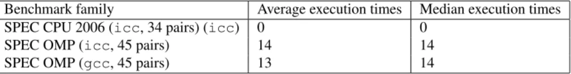
Table 1: Number of non statistically significant speedups in the tested benchmarks

Here the tool says that:

1. The probability that icc 11.0 beats gcc 4.1.3 (produces a speedup of the median execution time) on a randomly selected benchmark belongs to the interval [0.621; 0.861];

2. If this probability confidence interval is not tight enough, and if the user requires a confidence interval with a precision ofr = 5%, then the user has to make experiments on a minimal number of randomly selected benchmarksb = 281 !

6.4 The impact of the SpeedupTest protocol over some observed speedups

In this section, we give a synthesis of our experimental data to show that some observed speedups (that we call ”hand made”) are not statistically significant. In each benchmark family, we counted the number of non statistically significant speedups among those that are ”hand made”. Table 1 gives a synthesis. The first column describes the benchmarks family, with the used compiler and the number of observed speedups (pairs of samples). The second column provides the number of non statistically significant speedups of the average execution times. The last column provides the number of non statistically significant speedups of the median execution times.

As observed in the table, we analysed 34 pairs of samples for the SPEC CPU 2006 applications compiled with icc. All the observed speedups are statistically significant. When the program execution times are less stable, such as in the case of SPEC OMP 2006 (as highlighted in [1]), some observed speedups are not statistically significant. For instance, 14 speedups of the average execution times (among 45 observed ones) are not statistically significant (see the third line of Table 1). Also, 13 observed speedups of the median execution times (among 45 observed ones) are not statistically significant (see the last line of Table 1).

7 Related work and discussion

7.1 Observing execution times variability

The literature contains some experimental research highlighting that program execution times are sometimes increas-ingly variable or unstable. In the article of raced profiles [14], the performance optimisation system is based on observing the execution times of code fractions (functions, and so on). The mean execution time of such code fraction is analysed thanks to the Student’s t-test, aiming to compute a confidence interval for the mean. This previous article does not fix the data input of each code fraction: indeed, the variability of execution times when the data input varies cannot be analysed with the Student’s t-test. Simply because when data input varies, the execution time varies inher-ently based on the algorithmic complexity, and not on the structural hazards.

Program execution times variability has been shown to lead to wrong conclusions if some execution environment parameters are not kept under control [15]. For instance, the experiments on sequential applications reported in [15] show that the size of Unix shell variables and the linking order of object codes both may influence the execution times. Recently, we published in [1] an empirical study of performance variation in real world benchmarks with fixed data input. Our study concludes three points: 1) The variability of execution times of long running sequential applications

(16)

the samples of execution times do not follow a Gaussian distribution, which means that the Student’s t-test, as well as mean confidence intervals, cannot be applied on small samples.

7.2 Program performance evaluation in presence of variability

In the field of code optimisation and high performance computing, most of the published articles declare observed speedups as defined in Sect. 2. Unfortunately, few studies based on rigourous statistics are really conducted to check if the observations of the code performance improvements are statistically significant or not.

Program performance analysis and optimisation may rely on two well known books that explain digest statistics to our community [5, 8] in an accessible way. These two books are good introductions for doing fair statistics for analysing performance data. Based on these two books, previous work on statistical program performance evaluation have been published [16]. In the later article, the authors rely on the Student’s t-test to compare between two average execution times (the two sided version of the student t-test) in order to check ifµX 6= µY. In our methodology, we

improve the previous work in two directions. First, we conduct a one-sided Student’s t-test to validate thatµX> µY.

Second, we check the normality if small samples and the equivalence of their variances (using the Fisher’s F-test) in order to use the classical Student’s t-test instead of the Welch’s variant.

In addition, we must note that [5, 8, 16] focus on comparing between the mean execution times only. When the program performances have some extrema values (outliers), the mean is not a good performance measure (since the mean is sensitive to outliers). Consequently the median is usually advised for reporting performance numbers (such as for SPEC scores). Consequently, we rely on more academic books on statistics [6, 7, 9] for comparing between two medians. Furthermore, these fundamental books help us to understand mathematically some common mistakes and misunderstanding of statistics that we report in [3].

A limitation of our methodology is that we do not study the variations of the execution times due to changing the program’s input. The reason is that the variability of execution times when the data input varies cannot be analysed with the statistical tests as we did. Simply because when the data input varies, the execution time varies inherently based on the algorithmic complexity (intrinsic characteristic of the code), and not based on the structural hazards of the underlying machine. In other words, observing distinct execution times when varying data input of the program cannot be considered as hazard, but as an inherent reaction of the program under analysis.

8 Conclusion

The community of program performance evaluation and their optimisation techniques suffer from a lack of rigourous statistical evaluation methodology. This article treats the problem by defining a rigorous statistical protocol allowing to consider the variations of program execution times. The variation of program execution times is not a chaotic phe-nomena to neglect or to smooth; we should keep it under control and incorporate it inside the statistics.

Compared to [5, 8], the Speedup-Test methodology analyses the median execution time in addition to the average. Contrary to the average, the median is a better performance metric because it is less sensitive to outliers and is more appropriate for skewed distributions: this explains why the SPEC benchmark organisation advocates for it [4]. Sum-marising the observed execution times of a program with their median also allows to evaluate the chance to have a faster execution time if we do a single run of the application. Such performance metric is closer to the feeling of the users in general. Additionally, the Speedup-Test protocol is more cautious than [5, 8] because it checks the hypothesis on the data distributions before applying statistical tests.

The Speedup-Test methodology analyses the distribution of the observed execution times. For declaring a speedup for the average execution time, we rely on the Student’s t-test under the condition thatX and Y follow a Gaussian distribution (tested with Shapiro-Wilk’s test). If not, using the Student’s t-test is admitted but the computed risk level

(17)

α may still be inaccurate if the underlying distributions of X and Y are too far from being normally distributed. For declaring a speedup for the median execution time, we rely on the Wilcoxon-Mann-Whitney’s test. Contrary to the Student’s t-test, the Wilcoxon-Mann-Whitney’s test does not assume any specific distribution of the data, except that it requires thatX and Y differ only by a shift location (that can be tested with the Kolmogorov-Smirnov’s test).

We conclude with a short discussion about the appropriate risk level we should use in practice. Indeed, there is not a unique answer to this crucial question. In each context of code optimisation we may be asked to be more or less confident in the statistics. In the case of hard real time applications, the risk level must be low enough (less than 5% for instance). In the case of soft real time applications (multimedia, mobile phone, GPS, etc.), the risk level can be less than 10%. In the case of desktop applications, the risk level may not be necessarily too low. In any situation, the used risk level must be declared publicly in conjunction with the statistical significance.

References

[1] Mazouz A, Touati SAA, Barthou D. Study of Variations of Native Program Execution Times on Multi-Core Architectures. International Workshop on Multi-Core Computing Systems (MuCoCoS). IEEE: Krakow, Poland, 2010.

[2] Hennessy JL, Patterson DA, Goldberg D. Computer Architecture: A Quantitative Approach. Morgan Kaufmann, 2002. ISBN-13: 978-1558605961.

[3] Touati SAA, Worms J, Briais S. The Speedup-Test. Technical Report, University of Versailles Saint-Quentin en Yvelines Jan 2010. http://hal.archives-ouvertes.fr/inria-00443839.

[4] Standard Performance Evaluation Corporation. SPEC CPU 2006. URL http://www.spec.org/.

[5] Jain R. The Art of Computer Systems Performance Analysis : Techniques for Experimental Design, Measurement,

Simulation, and Modelling. John Wiley and Sons, inc.: New York, 1991. ISBN-13: 978-0-471-503361.

[6] Saporta G. Probabilit´es, analyse des donn´ees et statistique. Editions Technip: Paris, France, 1990. ISBN 978-2-7108-0814-5.

[7] Brockwell PJ, Davis RA. Introduction to Time Series and Forecasting. Springer, 2002. ISBN-13: 978-0387953519.

[8] Lilja DJ. Measuring Computer Performance: A Practitioner’s Guide. Cambridge University Press, 2000. ISBN-13: 978-0521641050.

[9] Hollander M, Wolfe DA. Nonparametric Statistical Methods. Wiley-Interscience, 1973. ISBN-13 978-0-471-190455.

[10] Conover WJ. Practical Nonparametric Statistics. John Wiley: New York, 1971. ISBN-13: 978-0-521-646703. [11] Brown LD, Cai T, DasGupta A. Interval Estimation for a Binomial Proportion. Statistical Science 2001;

16(2):101–133. With comments and a rejoinder by the authors.

[12] Feller W. An introduction to probability theory and its applications, vol. 1. John Wiley and Sons, Inc., 1968. Third edition, ”ISBN-13:978-0471257080”.

[13] Team RDC. R: A Language and Environment for Statistical Computing. 2008.

[14] Leather H, O’Boyle M, Worton B. Raced Profiles: Efficient Selection of Competing Compiler Optimiza-tions. Conference on Languages, Compilers, and Tools for Embedded Systems (LCTES ’09), ACM

(18)

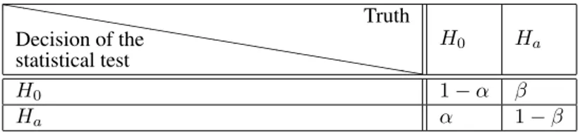
SIG-hh hh hh hh hh hh hh hh hh hh Decision of the statistical test Truth H0 Ha H0 1 − α β Ha α 1 − β

Table 2: The two risk levels for hypothesis testing in statistical and probability theory. The primary risk level (0 < α < 1) is generally the guaranteed level of confidence, while the secondary risk level (0 < β < 1) is not always guaranteed

[15] Mytkowicz T, Diwan A, Sweeney PF, Hauswirth M. Producing wrong data without doing anything obviously wrong! ASPLOS, 2009.

[16] Georges A, Buytaert D, Eeckhout L. Statistically rigorous Java performance evaluation. Proceedings of the

Twenty-Second ACM SIGPLAN Conference on OOPSLA, ACM SIGPLAN Notices 42(10), Montr´eal, Canada,

2007; 57–76.

A

Hypothesis testing in statistical and probability theory

Statistical testing is a classical mechanism to decide between two hypothesis based on samples or observations. Here, we should notice that almost all statistical tests have provedα risk level for rejecting an hypothesis only (called the null hypothesisH0). The probability1 − α is the confidence level of not rejecting the null hypothesis. It is not a

proved probability that the alternative hypothesisHais true with a confidence level1 − α.

By abuse of language, we say in practice that if a test rejectsH0 a null hypothesis with a risk levelα, then we

admitHathe alternative hypothesis with a confidence level1 − α. But this confidence level is not a mathematical one,

except in rare cases.

To have more hints on hypothesis testing, we invite the reader to study section 14.2 from [6] or section B.4 from [7]. We can for instance understand that statistical tests have in reality two kinds of risks: a primaryα risk, which is the probability to rejectH0 while it is true, and a secondaryβ risk which is the probability to accept H0 while

Hais true, , see Tab. 2. So, intuitively, the confidence level, sometimes known as the strength or power of the test,

could be defined as1 − β. All the statistical tests we use (normality test, Fisher’s F-test, Student’s t-test, Kolmogorov-Smirnov’s test, Wilcoxon-Mann-Whitney’s test) have only provedα risks levels under some hypothesis. We must say that hypothesis testing in statistics does not usually confirm a hypothesis with a confidence level1 − β, but in reality it rejects a hypothesis with a risk of errorα. By abuse of language, if a null hypothesis H0is not rejected with a risk

α, we say that we admit the alternative hypothesis Hawith a confidence level1 − α. This is not mathematically true,

because the confidence level of acceptingHais1 − β, which cannot be computed easily.

In this article, we use the abusive term confidence level for1 − α because it is the definition used in the R software to perform numerous statistical tests.