HAL Id: hal-01533710
https://hal.archives-ouvertes.fr/hal-01533710
Submitted on 6 Jun 2017HAL is a multi-disciplinary open access
archive for the deposit and dissemination of sci-entific research documents, whether they are pub-lished or not. The documents may come from teaching and research institutions in France or
L’archive ouverte pluridisciplinaire HAL, est destinée au dépôt et à la diffusion de documents scientifiques de niveau recherche, publiés ou non, émanant des établissements d’enseignement et de recherche français ou étrangers, des laboratoires
Model-based probabilistic reasoning for self-diagnosis of
telecommunication networks: application to a
GPON-FTTH access network
Serge Romaric Tembo Mouafo, Sandrine Vaton, Jean-Luc Courant, Stephane
Gosselin, Michel Beuvelot
To cite this version:
Serge Romaric Tembo Mouafo, Sandrine Vaton, Jean-Luc Courant, Stephane Gosselin, Michel Beu-velot. Model-based probabilistic reasoning for self-diagnosis of telecommunication networks: appli-cation to a GPON-FTTH access network. Journal of Network and Systems Management, Springer Verlag, 2017, 25 (3), pp.558 - 590. �10.1007/s10922-016-9401-0�. �hal-01533710�
Model-based probabilistic reasoning for
self-diagnosis of telecommunication networks:
application to a GPON-FTTH access network
S.R. Tembo
Orange Labs, 2 Avenue Pierre Marzin, 22300, Lannion, France S. Vaton
IMT Atlantique, 655 Avenue du Technopole, 29200, Brest, France J.L. Courant, S. Gosselin, M. Beuvelot
Orange Labs, 2 Avenue Pierre Marzin, 22300, Lannion, France Published in Journal of Network and Systems Management,
volume 25, issue 3, july 2017
Abstract
Carrying out self-diagnosis of telecommunication networks requires an understanding of the phenomenon of fault propagation on these networks. This understanding makes it possible to acquire relevant knowledge in order to automatically solve the problem of reverse fault propagation. Two main types of methods can be used to understand fault propagation in order to guess or approximate as much as pos-sible the root causes of observed alarms. Expert systems formulate laws or rules that best describe the phenomenon. Artificial intelli-gence methods consider that a phenomenon is understood if it can be reproduced by modeling. We propose in this paper, a generic proba-bilistic modeling method which facilitates fault propagation modeling on large-scale telecommunication networks. A Bayesian network (BN) model of fault propagation on GPON-FTTH (Gigabit-capable Passive Optical Network-Fiber To The Home) access network is designed ac-cording to the generic model. GPON-FTTH network skills are used to build structure and approximatively determine parameters of the BN model so-called expert BN model of the GPON-FTTH network. This BN model is confronted with reality by carrying out self-diagnosis of real malfunctions encountered on a commercial GPON-FTTH network. Obtained self-diagnosis results are very satisfying and we show how and why these results of the probabilistic model are more consistent with
the behaviour of the GPON-FTTH network, and more reasonable on a representative sample of diagnosis cases, than a rule-based expert system. With the main goal to improve diagnostic performances of the BN model, we study and apply EM (Expectation Maximization) algo-rithm in order to automatically fine-tune parameters of the BN model from real data generated by a commercial GPON-FTTH network. We show that the new BN model with optimized parameters reasonably improves self-diagnosis previously carried out by the expert Bayesian network model of the GPON-FTTH access network.
1
Introduction
Telecommunication operators make significant efforts to provide better qual-ity services to their subscribers. Telecommunication networks must be re-liable and robust to guarantee high availability of services to customers. Network management has become a central issue for telecommunication op-erators, which have triggered significant research in order to automate as much as possible numerous complex operations of network management, like fault management. Fault diagnosis is a central aspect of network fault management [1].
The main goal of fault diagnosis is to locate as quickly as possible fail-ures that degrade the quality of service provided to customers. Tradition-ally, fault diagnosis has been performed manually by an expert or a group of experts experienced in managing communication networks [1]. However, the development of telecommunication networks has increased the size and complexity of their architectures. Telecommunication networks have become large-scale complex distributed systems. A fault occurence spreads, trigger-ing other faults and alarms, which in turn trigger further faults and alarms. The consequence of both fault and alarm propagation is that a single root cause may result in a complex and distributed pattern of subsequent failures and their corresponding alarms [2]. This is especially true when multiple faults propagate simultaneously. Fault diagnosis has become too complex for humans, who can keep track of only a few hypotheses in their reasonings. Humans need a great deal of training to fully understand the fault propa-gation phenomenon in large-scale networks. Fault propapropa-gation is a complex phenomenon due to the dynamic, distributed and non-deterministic nature of telecommunication networks. A single fault may generate multiple alarms, and a single alarm may be triggered by several faults. Understanding fault propagation in order to automate fault diagnosis has become a critical issue
for operators. Understanding fault propagation is necessary to acquire rel-evant knowledge needed to perform self-diagnosis by automatically solving the problem of reverse fault propagation. This means using a configuration of alarms observed on the network to go back to the recent past in order to find their causal root explanations.
Two main types of methods can be used to understand fault propa-gation phenomenon in order to perform reverse fault propapropa-gation. Early self-diagnosis approaches of telecommunication networks, so-called expert systems, were rule-based. Expert systems [3] [4], encode specialized reason-ings on narrow diagnostic tasks in computer applications. Artificial science methods consider that a phenomenon is understood if it can be reproduced by modeling and simulation, for example. In this category, we may distin-guish model-based approaches [5], which develop reasonings based on an ex-plicit representation of the network. The blind methods based on machine learning algorithms, like artificial neural networks [6] [7], and case-based reasoning [8], infer diagnosis based on past experiences, without network modeling.
In [9], we proposed an artificial method which combines the advantages of model-based approaches and machine learning approaches. This generic probabilistic method of network modeling integrates two fields: a decision field and an artificial learning field. The decision field is based on Bayesian network probabilistic reasoning [10] [11] in order to deal with the uncertain-ties of fault propagation phenomenon. The artificial learning [12] field is introduced and brings self-reconfiguration capabilities to the generic model in order to deal with the dynamic nature of telecommunication networks.
This paper explains how and why probabilistic model-based methods improve self-diagnosis of telecommunication networks by solving main draw-backs of expert systems. We propose a Bayesian network (BN) model of fault propagation on GPON-FTTH (Gigabit-capable Optical Network-Fiber To The Home) [13] [14] access network. With our Python implementation of this probabilistic model, we carry out self-diagnosis on a large-scale com-mercial GPON-FTTH network. Parameters of the BN model, approximati-vately determined from GPON-FTTH network skills, are optimized by ap-plying EM (Expectation Maximization) algorithm from real GPON-FTTH network data.
work on fault diagnosis, as well as the comparison between expert systems and probabilistic model-based methods. We also explain in this section why and how a probabilistic model-based approach improves self-diagnosis of telecommunication networks compared to expert systems. Section 3 recalls basic concepts on Bayesian network models. Section 4 presents our de-signed generic probabilistic model, which facilitates fault propagation mod-eling on large-scale telecommunication networks. In Section 5, we apply and implement this generic method to GPON-FTTH access network modeling. Section 5 also presents and analyzes self-diagnosis results of our implemen-tation compared with those of a rule-based expert system. We study EM (Expectation Maximization) algorithm in Section 6 and apply it in Section 7 to automatically adjust parameters of the GPON-FTTH network model from real data generated by a commercial GPON-FTTH network. Section 7 also presents and analyses diagnosis results of the probabilistic model with optimized parameters comparativetely to diagnosis results of the previous GPON-FTTH network model. We conclude and present future works in Section 8.
2
Expert diagnosis systems and model-based
ap-proaches
Early self-diagnosis approaches were called expert systems. An expert diag-nosis system [3] [4] attempts to infer the cause of a problem from symptoms recognized in sensor data [2]. It is problem-solving software that embodies specialized reasonings on narrow diagnotic tasks, usually performed by a trained skilled human called an expert. The specialized reasonings can be formalized with rules, list of facts, logic predicates, etc. Inference engines are commonly based on forward-backward chaining algorithms. A review of diagnostic expert systems is available in [3] [4].
2.1 Rule-based expert systems
In the telecommunication industry, the most commonly used expert sys-tems are those that use rules to represent specialized diagnotic knowledge, so-called rule-based expert systems. A rule may be equated to a matching between observed symptoms and their corresponding causes. A rule takes the form IF < condition > T HEN < decision >. The condition may be evaluated directly if required data are available. Automated checks or tests on network components may also be necessary to evaluate the
con-dition. These tests increase the load of network components and generate additional network management traffic. If there are missing data, the con-dition cannot be evaluated and no decision can be taken. The decision can be the final diagnosis, i.e. the so-called conclusion, or the search for a more appropriate rule by using the rule inference engine. The inference engine has the ability to recognize input facts and infer output faults by searching for the most suitable rules to the recognized facts. Diagnosis computing fol-lows a cycle of fact recognition and rule inference that ends when the most appropriate rule is found. If some facts cannot be recognized due to missing data, the diagnosis computing cycle is interrupted and the expert system does not produce a decision.
Fault propagation in telecommunication networks is naturally a dynamic, distributed and non-deterministic phenomemon. This means that it is very difficult for human experts to design a set of rules which covers all possible situations that may occur on the network. Humans can keep track of only a few hypotheses in their reasonings and need a long training period called an expertise period to fully understand fault propagation on a network seg-ment. But despite these significant efforts to fully master the network, there are always unforeseen situations which require an extension of the expertise period. The set of rules designed by human experts can become obsolete if the new rules designed to cover an unforeseen situation require the modi-fication of old rules. Rule-based expert systems suffer from this paradigm, referred to as the knowledge acquisition bottleneck that make them very difficult to maintain and unsuitable to carry out self-diagnosis of large-scale telecommunication networks. An expert system is a static and deterministic approach inappropriate to solving the non-deterministic problem of reverse fault propagation in large-scale telecommunication networks.
2.2 Model-based approaches
Contrary to rule-based expert systems, model-based approaches no longer encode specialized reasonings on narrow diagnostic tasks. Model-based approaches use specialized knowledge about the network to build an ex-plicit, structured representation of network topology and network behavior. Model-based diagnostic approaches [15] [16] [17] [18] [19] [20] develop rea-sonings based on explicit, formal representation of network structure and network behavior. Network structure describes the network architecture. Network behavior describes the process of alarm propagation and alarm correlation [21]. Network structure and network behavior are then
mod-eled [5]. The obtained model is the support of reasoning algorithms which must be designed. Since reasonings are carried out on a model of the net-work, model-based approaches cover more situations than expert methods. They have the ability to deal with new problems or unforeseen situations, although their performance may degrade in these cases. Model-based ap-proaches are easier to maintain than expert systems. The model can be designed in a modular or incremental fashion, facilitating updates as new knowledge about the network is acquired.
The term self-modeling is recently used in the literature to indicate a model-based approach whose the model is built automatically. In [2] a self-modeling method based on patterns describing in generic manner de-pendencies among resources used by an IMS (IP Multimedia Subsystem) service is proposed. A pattern is based on a Bayesian network, it is built offline, automatically located and instantiated online when a fault occurs in a given IMS service. In [22] a similar self-modeling method applied in the context of SDN (Sofware Defined Network) and NFV (Network Functions Virtualization) is proposed. It is based on templates which model SDN elements. An algorithm parses the network topology given by the SDN con-troller and a template based on a Bayesian network, is instantiated with eventually additional dependencies. A Bayesian network formalism is also used in [23], to model the propagation of a crosstalk attack in an optical network architecture. The purpose of this work is to bring and evaluate resiliency of optical network architectures under in-band crosstalk attacks. In [24], a fault propagation model based on petri network is developped, such that places on petri network represent fault and transitions represent dependencies between fault. Transitions are eventually labeled by the corre-sponding alarm pattern. The diagnosis amounts to compute the most likely path given a sequence of observed alarms. Note that in above examples, the model is graphic. But, the model can be analytic. In [25], analytics models and monitoring metrics are used to locate physical layer impairment in WDM (Wavelength Division Multiplex) optical networks.
A model-based approach seems natural when relationships between ob-jects are graph-like and easy to obtain [1]. As we have seen in some above examples, the model can be probabilized in order to deal with uncertainties related to the non-deterministic nature of fault propagation.
However, it is quite difficult to build a model close enough to the struc-tural and functional reality of the network, while maintaining a high enough
level of abstraction to make the model independent of the various engineer-ing techniques implemented in telecommunication networks. In addition, the built model is reduced to a static image of the network and may be-come rapidly obsolete when the network changes. In [9], we have proposed a probabilistic generic model which embeds modularity and extensibility properties in order to facilitate self-reconfiguration of the model when the network changes.
2.3 Comparison between rule-based expert systems and a probabilistic model-based approaches
Table 1 summarizes the comparison between rule-based expert systems and probabilistic model-based approaches. We note that all the drawbacks of rule-based expert systems are solved by probabilistic model-based ap-proaches.
Table 1: Comparison between rule-based expert systems (RES) and proba-bilistic model-based approaches (PMA).
Properties RES PMA
Scalability No Yes
Maintenance Heavy Easy
New problems No Yes
Uncertainty No Yes
Missing data No Yes
Ambiguous data No Yes
Scope Narrow Large
Learning No Possible
The brittleness of rule-based expert systems, i.e., their inability to deal with unforeseen situations, is a consequence of their case-by-case reasoning lack-ing generalized reasonlack-ing capabilities. In addition to their ability to deal with uncertainty and missing data, probabilistic model-based approaches have a very wide scope of reasoning that makes it possible to make global or generalized intelligent analyses of all possible situations that may occur on the network. Therefore, contrary to a probabilistic model, a rule-based expert system does not scale and fails when it encounters new problems. Expert systems do not have the ability to learn from experiences acquired from early diagnostic tasks. However, a model-based approach with no learning capability is a static image of the network. In [9], we proposed a
probabilistic generic model-based approach which embeds modularity and extensibility, two useful properties for easy self-reconfiguration of the initial network model. This generic model is based on Bayesian networks formal-ism. So we first recall this formalformal-ism.
3
Basic concepts on Bayesian networks
A Bayesian network [10] [12] [11] is a probabilistic directed acyclic graphi-cal model which represents a set of random variables and their conditional dependencies via a directed acyclic graph (DAG). See Figure 1.
Figure 1: A simple Bayesian network of 6 random variables.
In a Bayesian network (BN) nodes represent random variables and edges represent dependencies. These random variables can be observations or measurements, latent variables or hypotheses for example. Each node is associated with a probability distributions that represent the distribution of the variable represented by the node, conditionally to the values of its parent nodes. These probabilities will be denoted as θi,j,k= P(Xi= k|pa(Xi) = j)
where this quantity stands for the probability that the value of node i is k given that the value of its set of parent nodes is j. A bayesian network en-codes dependencies and independencies between a set of random variables. Indeed, any two variables in a BN model are dependent if one belong to the Markov blanket of the other, otherwise there are independent. Note that the Markov blanket of a variable in a BN is the union between the set of parents and children of this variable and the set of other parents of children of this variable.
There are different definitions of what a BN is. Let B = (X1, X2, . . . , XN)
be the set of nodes of the BN. One possible definition is to state that the joint probability of random variables can be factored as the following product or
equivalently that the joint log-likelihood can be factored as a sum: P(B; Θ) = QNi=1P(Xi|pa(Xi)) =QNi=1θi,pa(Xi),Xi L(B; Θ) = log P(B) =PN
i=1log θi,pa(Xi),Xi
(1)
Here the notation P(B; Θ) (respectively L(B; Θ)) makes explicit that the joint likelihood (respectively log-likelihood) depends on the set of parame-ters Θ = (θi,j,k)i,j,k. A BN embeds powerfull and efficient computational
ca-pabilities. For example, it is possible to compute the conditional probability of any random variable or subset of random variables given an observation of one or many other variables, without performing heavy computations like marginalization. Indeed, efficient inference algorithms use the structure of the BN. Let’s consider for example the fragment of a tree BN depicted by Figure 2.
Figure 2: Segment of a tree Bayesian network.
Assume we want to compute the conditional probability of values of the variable X given some observed variables in the BN. The sum-product algorithm developped in [10], compute such conditional probability BEL(x) given observations e−X collected in subgraph G−X containing the descendant nodes of X, and observations e+X from the rest of the tree, i.e, the subgraph G+X. BEL(x) = P(x|e+X, e − X) = [P(e + X, e − X)] −1 P(e+X, x, e − X) = αP(e−X|e + X, x)P(x|e + X) = αP(e−X|x)P(x|e + X) = αλ(x)π(x) (2)
where λ(x) = P(e−X|x), π(x) = P(x|e + X) and α = [P(e + X, e − X)] −1 is
normal-izing constant. See [10] for detailled expressions of λ(x) and π(x). The sum-product algorithm use the structure of the BN since Equation 2 is ver-ified because variables in G+X are conditionnally independent from those in G−X given X. This conditional independence is true only for BN with no disoriented loop, i.e, a BN in witch any variable X does not belong to the set of its descendants, e.g. X /∈ G−X.
For BN with disoriented loops like the BN depicted by Figure 1, a kindly simplification of such BNs, called junction tree, is proposed in [26] [27]. A juntion tree is equivalent to a BN and inference algorithm on a junction tree is independent of the structure of the initial BN. This means that inference algorithm on a junction tree is very suitable for large and complex structures of BNs. Construction of a junction tree and inference on this structure is discussed in the next section which also describes our designed layered generic model for self-diagnosis of telecommunication networks.
4
A probabilistic generic model with self-reconfiguration
capabilities
The generic model is based on a very simple principle: modeling the behavior of a telecommunication network amounts to modeling the behavior of the components that make it up. The generic model can be applied to any distributed system for self-diagnosis purposes.
4.1 Description of the generic model
Each network component Ei is modeled by two Directed Acyclic Graphs
(DAG). One DAG, L2Ni, models local fault propagation on the component
in question (see Figure 3). Another DAG, L1Ni, models distributed fault
propagation between this component and components which are connected to it. Distributed fault propagation occurs between linked network compo-nents. The two DAGs L2Ni and L1Ni share some common variables. By
separating local fault propagation modeling from distributed fault propa-gation modeling, the generic model also models network topology. In [9], we discussed the roles of layer 1 agents cL1A, rL1A, layer 2 agents cL2A,
rL2A and layer 3 agents cL3A, rL3A (see Figure 3). We call layer 1 node,
a DAG L1Ni representing the network component Ei. We call layer 2 node,
Figure 3: The 3-Layered Generic Model
The generic model has three layers. Layer 1 models the network topol-ogy as well as distributed fault propagation between linked network com-ponents. Any node Ei of this layer is represented by a Directed Acyclic
Graph (DAG) noted L1Ni which embeds distributed dependencies between
the network component Ei and its neighbors. Note that i ∈ {1, . . . n} where
n is the number of network components of the telecommunication network modeled. Distributed dependencies model fault propagation between linked network components. For example, the Figure 4 shows a very simple model based on the generic model. It is the model of a network segment of three components connected under a bus topology. In Figure 4, layer 1 node L1N2
contains distributed dependencies between E1 and E2 and between E3 and
E2.
Layer 2 models local fault propagation on each network component. For example, in Figure 4, DAGs L2N1, L2N2 and L2N3 respectively model local
Figure 4: A simple example of the 3-Layered Generic Model.
L2N2 is connected to layer 2 DAGs L2N1 and L2N3 through layer 1 DAG
L1N2. The distributed nature of a telecommunication network introduces
mutual dependencies between linked network components. These mutual dependencies lead to undirected loops between some variables of the BN model. For example in Figure 4, layer 2 DAG L2N1 contains the local
undirected loop [A, B, D, C, A] on network component E1. In Figure 4, the
undirected loop [C, D, G, H, I, D, C] is distributed between components E1
and E2. Gr = n [ i=1 [L2Ni∪ L1Ni] (3)
Layer 3 is the junction tree representation [26] [27] [28] [11] of layer 1 and layer 2, i.e, the junction tree of the Bayesian network Gr defined by Equa-tion 3. We call layer 3 node, a clique Cp of the junction tree. As every
junction tree, layer 3 satisfies the running intersection property which en-sures that, the intersection Cp ∩ Cq is a subset of every clique and
sepa-rator of cliques on the path between Cp and Cq. For example, in Figure
separators {GD}, {GO} and {GM } which form the path between cliques {GDBC} and {GKM L}.
Note that, layer 1 and layer 2 are useful for the self-reconfiguration field of the generic model, since they provide useful modularity and extensibility properties. Layer 3 is useful for the decision field of the generic model since inference can be easily done in this layer, regardless of network topology complexity at layer 1 and network behavior complexity at layer 2. See [9] for more details.
The fault propagation model on a large-scale telecommunication network of n components is decomposed in 2n sub DAGs, interconnected. This de-composition brings useful, easy self-reconfiguration properties to the model, modularity and extensibility [9]. Therefore, the fault propagation model of a large-scale telecommunication network can be build incrementally, network component by network component. The model can easily follow changes in network topology like adding or removing a network component. The im-portant consequence is that we can start the network modeling by building a simple initial model from prior knowledge on a network segment. This initial model can be easily extended in order to take into account another network segment on which we recently acquired some knowledge about their behavior.
We introduced in [9] the specification of a reconfiguration protocol in order to automate the addition of a new network component into the initial network model or the removal of a network component from the current network model.
4.2 Construction of the junction tree
Consider the directed acyclic graph Gr defined by Equation 3. The fisrt step to build a junction tree that forms layer 3, is to moralize DAG Gr = (V e, Ed) where V e is the overall set of layer 2 nodes and Ed is the edges between them. The moral graph Gm = (V e, Em) of Gr is obtained by Equation 4 where Em is the set of edges of the moralized graph Gm.
(u, v) ∈ Em ⇐⇒ [(u → v) ∈ Ed] ∨ [(v → u) ∈ Ed]
∨ [∃w ∈ V e | u, v ⊂ parent(w)] (4)
moralized graph Gm. We note ζ the set cycles of Gm, ve(C) the set of vertices of a cycle C ∈ ζ, |ve(C)| the number of vertices of C and ed(C) the set of edges of the cycle C. The chordal graph Gc is defined by Equation 5.
(u, v) ∈ Ec ⇐⇒ [(u, v) ∈ Em] ∨ ∃C ∈ ζ with |ve(C)| > 3
such that [u, v ∈ ve(C) ∧ (u, v) /∈ ed(C)] (5)
Note that the quality of the triangulation largely determines the effi-ciency of the inference algorithm on junction tree. Triangulation is an opti-mization NP-hard problem. Indeed, an optimal triangulation is that which adds the smallest number of chords in the moralized graph, so-called mini-mum fill-in triangulation. In [29], a minimini-mum fill-in triangulation algorithm is proposed.
The third step to build a junction tree is to compute the maximal weighted spanning tree of the trianguled graph Gc. The maximal span-ning tree of the graph Gc is a subgraph that is a tree consisting of the subset of edges which together connect all cliques of Gc, while maximizing the total sum of weights on the edges. The weight is the size of the inter-section between adjacent cliques, i.e, the number of layer 2 nodes shared by adjacent cliques. The maximal spanning tree of an undirected graph can be computed using the Kruskal algorithm.
4.3 Diagnostic computations of the generic model
Layer 3 is the junction tree representation of the large bayesian network Gr obtained by combining layer 1 and layer 2 as shown by Equation 3. This means that layer 3 is sufficient to compute diagnostic decisions using, for example, the well-known exact inference algorithm on a junction tree [26] [27]. In Figure 3, layer 3 nodes Cp, Cq, Spq are respectively the cliques Cp
and Cq of the junction tree and their common separator Spq. A layer 3 node
is a compound variable of some layer 2 nodes. At initialization, a clique Cp
has the potential φCp and a separator Spq has the potential φSpq as follows:
φCp =
O
X∈Layer2,X∈Cp,pa(X)⊂Cp∨pa(X)=∅
P(X|pa(X))
φSpq = 1
(6)
We note pa(X), the parent set of layer 2 node X. The potential φCp of a layer 3 node Cp represents the joint conditional probability of the
layer 2 nodes that compose it. We recall that the product of distributions P(Xi|pa(Xi)) of Equation 6 is not a matrix product but a tensor product
of functions. Indeed, a distribution P(Xi|pa(Xi)) is a function of variables
(Xi, pa(Xi)).
We call evidence e, a configuration or a combinaison of values taken by a subset E of some layer 2 nodes. Let E = {X1, X2, . . . , Xt} and E ⊂ Layer2,
then e = {x1, x2, . . . , xt} such that xi for i ∈ {1, . . . , t} is a value taken by
the layer 2 node Xi ∈ E.
The diagnostic decisions computed at layer 3 are based on evidence prop-agation on a junction tree. This algorithm starts by recomputing the initial potential of each observed clique or layer 3 node by setting observed layer 2 nodes belonging to this clique. A clique is observed if at least one layer 2 nodes of this clique is observed. After that, the evidence propagation algo-rithm essentially consists to update the potentials of any couple of adjacent cliques. Assume Cp, Cq to be neighboring layer 3 nodes with their common
separator Spq(see Figure 3). The algorithm updates the potentials of cliques
Cp and Cq toward the separator Spq.
φ∗Spq = X Cp\Spq φ∗Cp (7) φ∗Cq = φCq φ∗S pq φSpq (8)
Assume for example that the potential of Cp has been already updated
and the potential of Cq has not yet been updated, i.e, the propagation
algo-rithm has already reached clique Cp but not yet the adjacent clique Cq. The
evidence propagation algorithm proceeds in two steps. Firstly, the potential of the separator Spq is updated by applying the marginalization operation
of Equation 7. Secondly, the potential of the clique Cq is updated by the
product of Equation 8. The notation Cp \ Spq represents the set of layer
2 nodes of clique Cp which does not belong to separator Spq. We say that
clique Cqabsorbs evidence from Cp [21] or that clique Cp brings evidence to
Cq.
Updating operations of potentials of cliques and separators are carried out in two recursives stages. The first stage called collect is initiated by collecting evidence from leave cliques to root cliques. This assumes that we arbitrarily choose an orientation on the junction tree by designating some
pending cliques as leave cliques of the tree and the other pending cliques are therefore root cliques of the tree. Root clique and leaves cliques respec-tively denote cliques with no predecessor and cliques with no successor in the junction tree according to orientation choosen. Collection of evidence to a clique Cp is done by collecting evidence to all children of Cp followed
by absorption of evidences from each child. The second stage is initiated by distributing evidence from root cliques to leave cliques. Distribution of evidence from a clique consists to bring evidence to each child followed by distribution of evidence from the child.
Note that the update operations of the potentials of layer 3 nodes are carried out by an agent called computing Layer 3 Agent cL3A. The cL3A
updates the potential of each layer 3 node when it receives evidence (ob-served layer 2 nodes) from its layer 2 counterpart called cL2A. When cL2A
receives updated layer 3 node potentials, it computes the marginals (beliefs) of layer 2 nodes. These two agents may communicate using a simple mech-anism like shared memory through an interface between layer 2 and layer 3, which we call the L2-L3 Interface (see Figure 5).
Figure 5: Communication between layer 2 and layer 3 for belief updating of layer 2 nodes
After updating the potential of all layer 3 nodes, the updated potential φ∗Cp of the clique Cp is the joint probability of layer 2 nodes belonging to
this clique and evidence e.
φ∗Cp = P(Cp, e) (9)
This means that the likelihood P(e) of evidence e and the conditional marginal probability P(X|e) of a layer 2 node X given e, can be computed
by applying Equation 10. P(e) = X Cp φ∗Cp and P(X|e) = X Cp\X P(Cp|e) (10)
Where P(Cp|e) = φ∗Cp/P(e) is the joint probability of layer 2 nodes
be-longing to the clique Ci. The intersection property verified by a junction tree
ensures coherence between updated potentials, i.e, the conditional marginal of a layer 2 node X given evidence e, is the same regardless of the clique Cp
on which the marginalization operation is made. The most probable state of the layer 2 node X that is consistent with evidence, is the one that has the highest conditional marginal probability. The most propable state of layer 2 root nodes give us the diagnosis decision. Note that there is an al-ternative approach to finding the diagnosis without performing summation operations on updated potentials. With this approach, the diagnosis r∗, is computed from the most probable explanation w∗, of evidence as follows: w∗=S
C∈Layer3wC∗ such that φC(w∗C) = maxwCφC(wC), where wC is a con-figuration of layer 2 nodes belonging to layer 3 node C and w∗C maximizes the potential φC of C. Diagnosis r∗ is the most probable configuration of
layer 2 root nodes defined by r∗ = w∗ \ i∗, where i∗ is the most probable
configuration of non-root layer 2 nodes consistent with the evidence.
5
Case study: self-diagnosis of the GPON-FTTH
access network
In this section, we apply the generic model to build an initial probabilistic model of the GPON-FTTH network. We force this model of self-diagnosis to confront reality by carrying out fault diagnosis on an operating GPON-FTTH network. The diagnostic results obtained with the probabilistic model are presented, analyzed and compared with those obtained by a rule-based expert system. Let us start with the presentation of the GPON-FTTH network and the probabilistic model-based approach for self-diagnosis of this network.
5.1 The GPON-FTTH access network
The GPON-FTTH access network has two main network components. The Optical Line Termination (OLT ) is located on the operator side, and the Optical Network Termination (ONT ) is located on the customer side, and
the OLT and ONT are connected through an Optical Distribution Net-work (ODN ), which is the optical infrastructure made of fibers and passive components like splitters. A Passive Optical network (PON ) is a point-to-multipoint link inside the ODN. A PON has a tree-like topology which connects an OLT with a maximum of 64 ONTs in our example (see Figure 6). Each ONT is connected to an RG (Residential Gateway) via an Eth-ernet link. Since there is no interaction between PONs in ODN, and all PONs have the same behavior, we modeled one single PON. This model can be replicated to any PON of a GPON-FTTH access network. All ONTs connected to the same PON temporally share the upstream optical channel of the PON. The downstream channel of the PON is a secured broadcasting channel.
Figure 6: GPON-FTTH network architecture
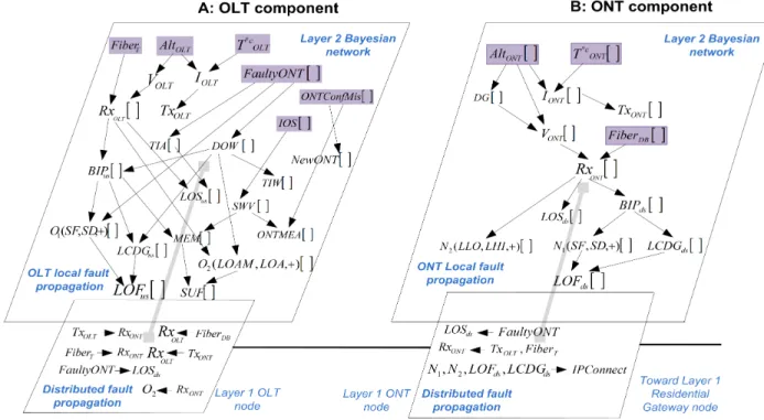
Figure 7.A depicts the model of OLT component for self-diagnosis pur-pose. As designed by the generic model, this component is modeled by two DAGs. One DAG called layer 2 DAG for local fault propagation and a layer 1 DAG for distributed fault propagation between OLT and ONT components. The two DAGs are connected since they have some common variables. Figure 7.B depicts the model of ONT component. The two models are connected since they share common distributed dependencies via layer 1 (see Figure 7). Figure 7 presents the application of the generic model for modeling the topology and behavior of a PON of the GPON-FTTH access network. The obtained model has two layer 1 nodes, i.e., the components OLT and ONT. Some variables called layer 2 nodes are vectors in order to respect the tree-like topology of a PON. Indeed such layer 2 nodes represent a particular value (for example an alarm, a counter or a scalar parameter) at the different ONTs of the PON. Each element i of the vector refers to ONT
Figure 7: The GPON-FTTH model based on the generic model.
number i in the PON. For reasons of simplicity, layer 3 is not depicted. We have three types of layer 2 nodes on Figure 7: faults or root causes, inter-mediate faults and alarms. The root causes are highlighted in Figure 7.
The transport optical fiber of the PON denoted by F iberT can take three
states. The OK state means that there is no transmission anomaly on this fiber. The AT and BR states mean respectively that the fiber is experienc-ing high attenuation or that the fiber is broken. The temperature of OLT denoted by Tc
OLT, is a continous variable that we discretize. The power
supply of OLT denoted by AltOLT may or may not be faulty. The node
F aultyON T denotes an ONT which transmits an upstream signal outside of its granted time slot, which may conflict with data sent by other ONTs on the PON and cause data disruption for a random set of ONTs, making the PON unusable. A FaultyONT can cause a Drift of Windows DOW . The component OLT raises a DOW [i] alarm when an ON T [i] transmits a signal beyond the time slot allocated to it. See ITU-T G984.3 [13] [14] for more details. We note i ∈ {1, ..., 64} the position of this ON T on the PON.
The Software Version SW V [i] alarm means that there is an incompati-bility between the Image Operating System (IOS) of ON T [i] and those of the OLT. The node ON T Conf M is (ONT Configuration Mistake) denotes a configuration error during ONT provisioning. The OLT transmitted power T xOLT is regulated by the bias current IOLT. This leads to the local
de-pendency IOLT −→ T xOLT. The OLT received power RxOLT[i] from an
ON Ti depends on the OLT voltage VOLT and the state of the feeder fiber
F iberT. The OLT received power of ON Ti also depends on the state of the
drop fiber denoted by F iberDB[i] and the transmitted power of this ON Ti
denoted by T xON T[i]. Note two local dependencies (F iberT −→ RxOLT,
VOLT −→ RxOLT) and two distributed dependencies (F iberDB −→ RxOLT,
T xON T −→ RxOLT). Note in Figure 5 that the distributed dependencies
are part of the edges of the layer 1 OLT, node which is a DAG as designed in the generic model.
The Bit Interleaving Parity denoted by BIP us[i] depends on the Bit Er-ror Rate BER of an upstream data transmission between an ON Ti and OLT.
A poor upstream signal reception can cause bit errors, leading to the local dependency RxOLT −→ BIP us. Upstream transmission bit errors impact
the quality of the signal received by OLT, which may raise some alarms re-lated to signal quality like SD (Signal Degraded), SF (Signal Fail), LCDG (Loss of GEM Channel Delineation) and M EM (Message Error Message). See ITU-T G984.3 [13] recommendation for more details.
When the received power RxON T[i] of an ON Ti is less than a
preconfig-ured minimum threshold, this ONT raises the (Level Low) LLO[i] alarm. The (Level High) LHI[i] alarm is raised by ON Tiwhen RxON T[i] is greater
than a preconfigured maximum threshold. For simplicity and because the LEV ELLO alarm denoted by LLO and the LEV ELHI alarm denoted by LHI can not be observed simultaneously, we have considered them to be states of the layer 2 node called N2(LLO, LHi, +). The state denoted by +
means that there is no LLO or LHI alarm observed. The received power RxON T[i] depends on voltage VON T[i], the state of drop fiber F iberDB[i], the
state of feeder fiber F iberT of the PON and the transmitted power T xOLT of
OLT. Note the local dependencies VON T −→ RxON T, F iberDB −→ RxON T
and the distributed dependencies T xOLT −→ RxON T, F iberT −→ RxON T.
Now, suppose we need to extend this model by adding another layer 1 node: a Residential Gateway RG node, for example (see Figure 6). An
RG is a home network component that provides services to customers. It is not a GPON-FTTH network component, but adding it to the model will enable the model to correlate the faults and alarms of the GPON-FTTH network with customer service malfunctions. For example, in Fig-ure 5, we can make such a correlation with the distributed dependency N1, N2, LOFds, LCDGds −→ IP Connect, where IP Connect denotes the
Internet access service provided by an RG. To add the layer 1 RG node, we will need only to specify and quantify the uncertainties of its local de-pendencies and distributed dede-pendencies with the layer 1 ONT node, which already exists in the model.
5.2 Parameters estimation of the GPON-FTTH network model
In the last subsection, we have showed how we can use skills about GPON-FTTH network to design a fault propagation model of this network. Here, we also show how these skills can be used to turn this model into a bayesian network by approximatively determining the parameters of this model, i.e, a probability distribution of each layer 2 node conditionally to its parents, which aims to quantify uncertainties on dependencies. Obviously, it is more pratice to adjust the parameters of a statistical model by applying machine learning techniques from a dataset. But, our choice to use expert knowledge about GPON-FTTH network, in order to find an estimation of parameters, is motivated by the fact that machine learning algorithm for parameters estimation of a bayesian network model is based on maximum likelihood principle of the dataset. This algorihm requires an initial value of parame-ters vector to perform estimation from incomplet dataset as it is often the case for a telecommunication network dataset. This initial value should not be aberrant, it must be quite realistic to hopefully avoid problems related to local optimum of the likelihood of data. Therefore parameters approx-imatively determined with GPON-FTTH network skills in this subsection, so-called expert parameters can later serve as initialization point to an algo-rithm such that EM (Expectation Maximization) [30] [31] which can there-fore adjust them automatically from GPON-FTTH network data.
Consider a layer 2 node Xi of the GPON-FTTH model depicted by
Fig-ure 7. We note θi,j,k = P(Xi = k|pa(Xi) = j) the probability that the
variable Xi takes the value k when the combinaison of values taken by
its parents is j. We propose to approximatively determine the conditional probability distribution θi = P(Xi|pa(Xi)), based on GPON-FTTH network
develop a structured reasoning consistent with the behavior of the GPON-FTTH network. We recall in the words of Glenn Shafer (a pioneer of the theory of probability applied to artificial intelligence) that ”Probability is not really about numbers; it is about the structure of reasoning”. For our problem, we search two orders of magnitude. An order of magnitude be-tween proportions of the vector θi,j,•, for all possible values of k, with the
constraintsP
kθi,j,k = 1 and θi,j,k ∈ [0, 1]. An order of magnitude between
the probabilities of the vector θi,•,k, for all possible values of j. In order
words, we search an order of magnitude between elements of each lign and an order of magnitude between elements of each column of the 2-dimensions matrix θi = P(Xi|pa(Xi)). We illustrate with some examples below how
such magnitude orders can be determined based on GPON-FTTH network skills.
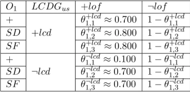
The first exemple concerns the estimation of conditional probability dis-tribution P(LOFus|O1, LCDGus). Table 2 represents this distribution. We
note +lof , the event of loss of data frame that is manisfested by the ob-servation of LOF (Loss Of Frame) alarm. ¬lof is the complementary of +lof event. On the upstream channel between OLT and one ONT, it is more probable that the loss of a data frame (+lof ) occurs when an error of delineation of frames (+lcd, loss of gem channel delineation) transmitted by this ONT occurs, than when OLT carry out frames delineation with-out error (¬lcd). This technical knowledge abwith-out GPON-FTTH network is represented by constraint 11 in which the event +e corresponds +lcd and the complementary ¬e of +e corresponds to ¬lcd, (see Table 2). Numerical values in this table are consistent with constraints 11, 12 and 13.
θ¬ep,q≤ θp,q+e for p = 1, q ∈ {1, 2, 3} (11) Futhermore, since transmission errors rate is more important when SF (Signal Fail) alarm is observed than when SD (Signal Degraded) alarm is observed, then it is more likely that loss of frames occurs when signal degradation level is high (SF ) than when it is medium (SD). We represent this information by constraint 12.
θ+ep,q≤ θ+ep,q+1
θ¬ep,q≤ θ¬ep,q+1 for p = 1, q ∈ {1, 2} (12)
Finally, we can say that it is more likely that a loss of frames occurs on the upstream channel when its two potential causes occurred, i.e, the
observation of a high or medium signal degradation via SFusalarm or SDus
alarm, and the observation of a frames delineation error via LCDGus, than
when only one of two potential causes occurred. So, we can also consider the constraint 13 (see Table 2).
θ1,2¬e ≤ θ+e1,3 and θ1,3¬e ≤ θ+e1,2 (13)
Table 2: The 2-Dimensions matrix that represents the conditional probabil-ity distribution P(LOFus|O1, LCDGus).
O1 LCDGus +lof ¬lof + θ+lcd1,1 ≈ 0.700 1 − θ+lcd1,1 SD +lcd θ+lcd1,2 ≈ 0.800 1 − θ+lcd1,2 SF θ+lcd1,3 ≈ 0.800 1 − θ+lcd1,3 + θ¬lcd1,1 ≈ 0.100 1 − θ¬lcd1,1 SD ¬lcd θ¬lcd1,2 ≈ 0.700 1 − θ¬lcd1,2 SF θ¬lcd1,3 ≈ 0.700 1 − θ¬lcd1,3
The conditional probabilities of the distribution P(LOFus|O1, LCDGus)
must satisfy the three constraints formalized by inequations 11, 12 and 13. In other words, these three constraints formalize GPON-FTTH net-works skills encoded in the distribution P(LOFus|O1, LCDGus). Table 2
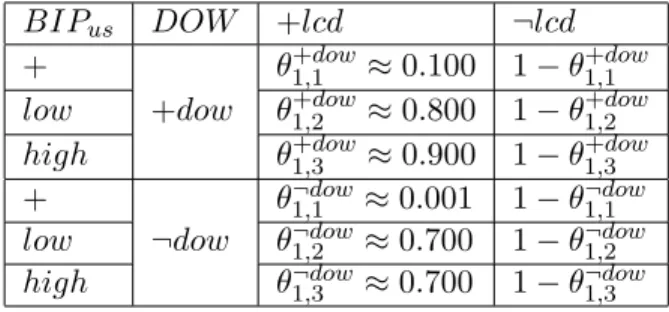
gives an approximative value of each conditional probability consistent with order of magnitude defined by these three constraints. The second ex-emple concerns the estimation of the conditional probability distribution P(LCDGus|BIPus, DOW). Table 3 shows how this distribution is
approx-imatively determined based on constraints 11, 12 and 13 on which event +e corresponds to event +dow and the complementary ¬e of +e corresponds to ¬dow. The first constraint expresses that, for any transmission errors rate, it is more probable that an error of frames delineation occurs (+lcd event) when a drift of slot transmission time is observed (+dow event), than when it is not the case (¬dow event). The second constraint 12 formalizes that, regardless of +dow event, the probability that an error of frames delin-eation occurs, increases with transmission errors rate BIPus. According to
the third constraint 13, it is more likely that an error of frames delineation occurs on the upstream channel when its two potential causes occurred, i.e, the observation of a drift of windown alarm, and a high or medium trans-mission errors rate, than when only one of two potential causes occurred.
Table 3: The 2-Dimensions matrix that represents the conditional probabil-ity distribution P(LCDGus|BIPus, DOW ).
BIPus DOW +lcd ¬lcd
+ θ1,1+dow≈ 0.100 1 − θ1,1+dow low +dow θ1,2+dow≈ 0.800 1 − θ1,2+dow high θ1,3+dow≈ 0.900 1 − θ1,3+dow + θ1,1¬dow ≈ 0.001 1 − θ1,1¬dow low ¬dow θ1,2¬dow ≈ 0.700 1 − θ1,2¬dow high θ1,3¬dow ≈ 0.700 1 − θ1,3¬dow
A similar probabilistic reasoning to those developped in Tables 2, 3 and constraints 11, 12 and 13 is used to approximatively determine the distribu-tion of each variable of the GPON-FTTH network model depicted by Figure 7. These distritutions turn the directed acylic graph Gr defined by Equa-tion 3 into a bayesian network (BN). Since the structure of the bayesian network Gr is designed by skilled humans on GPON-FTTH network, Gr is a causal bayesian network. Indeed, for humans, a simple and intelligible way to represent causes and effects relationships describing fault propagation, is a causal dependency graph. However if the structure had been learned by a machine learnig algorithm from a data sample, arrow between two variables will not necessarily express causality but rather correlation between them.
We have used this bayesian network (BN) model to perform self-diagnosis of the GPON-FTTH network. In order to validate and assess performances of self-diagnosis with the BN model, we have used two different approaches. A first approach described in [9] was to set up a physical testbed with a PON with two ONTs. Different faults were emulated, and alarms as well as counters were collected. The diagnosis of the root cause of alarms was performed with the BN approach. Seven usual fault scenarios were considered. Diagnosis results were inspected manually in order to assess their reliability. This demonstrated that self-diagnosis based on a BN model was a reliable and promising approach. In a second phase, the BN model is confronted with reality by carrying out self-diagnosis on an operating GPON-FTTH network.
5.3 Self-diagnosis results on an operating GPON-FTTH ac-cess network
We present and analyze in this section the network fault diagnosis results carried out by our application and implementation of the generic model to perform self-diagnosis of a GPON-FTTH network. The experiments were performed on an operating GPON-FTTH network on which we have con-sidered different PONs. For each PON concon-sidered, we call the ONT being tested, the first ONT of this PON, i.e., ON T1. The other ONTs connected
to this PON are called the neighbors of ON T1. We collected the alarms
raised by the operating PON network components, i.e., OLT and ONTs. We also read, if available, the values of counters BIPus, BIPds and scalar
parameters RxOLT, RxON T, T xOLT, T xON T, voltages VOLT, VON T, bias
cur-rent IOLT, ION T, temperatures TOLTc , TON Tc of OLT and ONTs connected
to the considered PON.
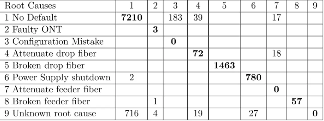
A database of 10611 real diagnosis cases collected by Orange on a com-mercial GPON-FTTH network in july-august 2015 was analysed. Two tools are compared: PANDA, the self-diagnosis tool based on the BN approach de-scribed in this paper, and DELC, a self-diagnosis tool based on deterministic decision rules. DELC is currently used to diagnose faults in the operational network. DELC is based on Drools, a business rules management system solution developed by the JBoss community, that provides a core business rules engine. We present and analyze quantified self-diagnosis results of a GPON-FTTH network carried out separately by DELC rule-based expert system and our probabilistic model-based tool PANDA. A 2-dimension con-fusion matrix depicted by Table 4 is used to compare the results obtained with each of the two methods.
In Table 4, each row of the confusion matrix is labelled by a diagnosis re-sult obtained with the expert system. Each column is labelled by a diagnosis result obtained with the probabilistic model-based approach. Although the probabilistic model simultaneously carries out the diagnosis of all ON T s connected to the PON being considered, we have limited the comparison to the diagnosis of only one ON T . That is because the expert system out-puts only the diagnosis of one ON T , namely the ON T under test, i.e., the ON T named ON T1 in our PON model. The comparison is made on 10611
diagnosis cases. Observations of each case are collected from an operating GPON-FTTH network. For each case, the expert system and the probabilis-tic model separately perform a diagnosis based on the same observations.
Table 4: A 2-dimension confusion matrix between the results of the rule-based expert system and the probabilistic model-rule-based system.
Root Causes 1 2 3 4 5 6 7 8 9
1 No Default 7210 183 39 17
2 Faulty ONT 3
3 Configuration Mistake 0
4 Attenuate drop fiber 72 18
5 Broken drop fiber 1463
6 Power Supply shutdown 2 780
7 Attenuate feeder fiber 0
8 Broken feeder fiber 1 57
9 Unknown root cause 716 4 19 27 0
In Table 4, bold numbers placed on the matrix diagonal represent cases for which the expert system and the model have given the same diagnosis result for ON T1consistent with the results supervised by the oracle
(GPON-FTTH network engineers). For example, as expected by oracle analysis of observations, we note 7210 cases, 3 cases, 72 cases, where the two methods have respectively concluded that no default is identified on the PON, the ON T under test is faulty and the drop fiber of this ON T is experiencing attenuation. See Table 4. We focus our analysis on cases placed outside the diagonal of the matrix, i.e, the cases for which diagnosis results of the two methods do not converge.
There are 183 cases for which the expert system is unable to detect a configuration mistake during ONT provisioning. The reason for this is simply that there is not yet expert rule that handles this situation. Table 5 shows the diagnosis of the probabilistic model for this simple situation.
Table 5: The PON has forty ONTs. The N ewON T [1] alarm is observed on ON T1. Counters and scalar parameters of all ONTs are nominal.
Root causes States Beliefs
ON T Conf iguration [OK, ¬OK] [0.020, 0.980]
We note 39 cases for which the expert system returns no default while the probabilistic model diagnoses that the drop fiber of ON T1 under test is
experiencing attenuation. In order to explain this difference, we looked very closely at the observations collected for these cases. Either the upstream
Table 6: The PON has forty ONTs. No alarm is observed. The upstream received power of ON T1 is non-nominal, i.e. node RxOLT[1] has low value.
The downstream received power of ON T1is not mesured, i.e, node RxON T[1]
is missing. Counters and scalar parameters of neighboring ONTs are nomi-nal.
Root causes States Beliefs
F iberDB1 [OK, AT, BR] [1.e-03, 0.93, 5.e-02] F iberDBi6=1 [OK, AT, BR] [0.92, 8.e-02, 2.e-06] F iberT [OK, AT, BR] [0.99, 2.e-09, 1.e-48]
received power or the dowstream received power of ON T1 is low, and other
is missing while the power levels of its neighbors are nominal. The expert rules do not clearly describe this situation, while the model does so naturally. Indeed, expert rule needs both upstream and downstream received powers to diagnose the state of the optical link, while probabilistic model is capable to deals with missing of one received power level since it make a global analysis of the PON. An instance of this case is described by Table 6. Note in Table 6 that the feeder fiber noted F iberT does not attenuate since power levels of
neighbors of ON T1 are nominal. Note that when power levels of neighbors
are also low, the probabilistic model understands that it is the feeder fiber of the PON shared by all ON T s which is experiencing attenuation (see Table 7). This last situation is encountered in 17 cases for which the expert system does not detect any fault. This situation also explains the 18 cases for which the expert system returns that the drop fiber is attenuating (when both RxOLT[1] and RxON T[1] are lows) while the model says us that it is
rather the feeder fiber which is experiencing attenuation.
Table 7: The PON has forty ONTs. No alarm is observed. The upstream received power of ON T1 is non-nominal, i.e. node RxOLT[1] has low value.
The downstream received power of ON T1is not mesured, i.e, node RxON T[1]
is missing. Received power levels of neighboring ONTs are non-nominal. Root causes States Beliefs
F iberDBi [OK, AT, BR] [0.62, 0.37, 2.e-06] F iberT [OK, AT, BR] [2.e-02, 0.97, 9.e-06]
There are 780 cases for which both the expert system and the probabilis-tic model diagnose that the power supply of ON T1 is down or faulty. See
and scalar parameters of the ON T in question, computed by the probabilis-tic model, enforce the belief that the power supply of this ON T is shut down or defective. The most probable state of the bias current of this ON T is I0, i.e., a null bias current. The voltage is null with a belief of 0.95. The
transmitted and received powers of this ON T have very low values, with a belief of 0.99.
Table 8: The PON has twenty ONTs. DG alarm is observed on ON T1, i.e.,
node DG[1] takes value 1. Counters and scalar parameters of ON T1 are
missing. Counters and scalar parameters of neighboring ONTs are nominal. Root causes States Beliefs
AltON T1 [OK, ¬OK] [0.001, 0.999] AltON Ti6=1 [OK, ¬OK] [0.999, 0.001]
Table 9: The most probable states of missing observations useful to detecting shutdown or defective power supply in table 8.
Root causes States Beliefs ION T1 [I0, I1] [0.95, 0.05] VON T1 [V0, V1] [0.98, 0.02]
RxOLT1 [Rx0, Rxl, Rxn] [ 0.99, 2.e-03, 1.e-03] RxON T1 [Rx0, Rxl, Rxn] [ 0.99, 4.e-03, 4.e-03] T xON T1 [Tx0, T xl, T xn] [ 0.99, 3.e-02, 3.e-03]
Confusion matrix depicted by Table 4 also shows 2 cases for which the model returns no default, while expert system said that power supply is down. This difference is due to the fact that the expert rule concludes that the power is down when the DG[1] alarm is observed. This narrow rule does not consider the situation where the DG[1] alarm is observed but the counters and scalars of ON T1 are still available and nominal. The model
clearly understands this situation and deduces that power supply of ON T1
is not down but it is going to be shut down, i.e., there is no default at this time. See Table 10.
The most significant cases for which the probabilistic model clearly out-performs the rule-based expert system are the cases for which the expert system has trouble computing the diagnosis due to missing observations or unforeseen situations, i.e., the situations not yet covered by the existing rules. For each of these cases the expert system returns unknown root cause,
Table 10: The PON has twenty ONTs. DG[1] alarm is observed on ON T1.
Counters and scalar parameters of ON T1 are nominal. Counters and scalar
parameters of neighboring ONTs are nominal. Root causes States Beliefs
AltON T1 [OK, ¬OK] [0.910, 0.090] AltON Ti6=1 [OK, ¬OK] [0.999, 0.001]
i.e., it is not able to output any conclusion, while the probabilistic model naturally computes the most probable diagnosis based on available observa-tions even if some of them are missing.
There are 716+4+19+27 cases for which the expert system fails because observations are not sufficient to run its rules, while the model uses the few available observations in order to complete the observations by infering the most probable states of useful missing observations. The diagnosis is then computed based on completed observations. For example, there are 19 cases for which the expert system fails to compute the diagnosis based on the ob-servation of the LEV ELLO[1] alarm with missing received power levels of ON T1. For each of these cases, the probabilistic model infers that the most
probable values of these received powers are very low, i.e, Rx0 in Table 12,
and deduces that the most probable explanation of the LEV ELLO[1] alarm is the drop fiber attenuation of ON T1. See Table 11. We also note among
these cases, 716 cases for which the expert system fails while the probabilis-tic model returns no default. This result may seem trivial, however it has a capital interest for a telecommunication operator. Indeed, this result indi-cates a nominal operation of the GPON-FTTH infrastructure and allows to deduce that the fault is certainly in the home network of the complaining subscriber. Therefore, this result allows operator to avoid triggering use-less interventions on GPON-FTTH infrastructure, but rather to intervene eventually on the home network of the subscriber. So, this result allows to reduce the number of technical interventions and save time and money to customer service of the operator.
Self-diagnostic results of the probabilistic model are more consistent with the behaviour of the GPON-FTTH access network, and more reasonable on a representative sample of cases, than the rule-based expert system. Note for example that for 7% of cases, the expert system fails, while the prob-abilistic model correctly computes a diagnosis. The principal explanation
Table 11: The PON has forty ONTs. The LEVELLO alarm is observed on ON T1, i.e., N2[1] = LLO. Upstream and downstream received power of
ON T1 are missing. Counters and scalar parameters of neighboring ONTs
are nominal.
Root causes States Beliefs
F iberDB1 [OK, AT, BR] [5.e-02, 0.94, 1.e-06] F iberDBi6=1 [OK, AT, BR] [0.91, 8.e-02, 1.e-06] F iberT [OK, AT, BR] [0.99, 2.e-021, 5.e-105]
Table 12: The most probable levels of missing received powers useful in detecting feeder fiber attenuation in table 11.
Nodes States Beliefs
RxOLT1 [Rx0, Rxl, Rxn] [ 0.88, 0.10, 0.02] RxON T1 [Rx0, Rxl, Rxn] [ 0.82, 0.17, 0.01]
of these differences is that the probabilistic model has a wide scope of rea-soning that allows it to make global or generalized intelligent analyses of situations. Doing so, the model covers unforeseen situations encountered by the rule-based expert system, which reasons case-by-case. Therefore the rule-based expert system lacks generalized reasoning capabilities.
Note that in tables above, the numbered root causes correspond to the final diagnosis decision. It is a podium of the most problable root causes that explains observations. This final diagnosis decision is computed from beliefs or posterior probabilities of all root causes of the GPON-FTTH model depicted in Figure 7. Beliefs of root causes are computed by the well-known algorithm of evidence propagation on the junction tree. To compute the fi-nal diagnostic decision from root cause beliefs, we proceed in two steps. We start the algorithm by finding the set R0 of root causes whose the beliefs
are not equally probable. This step aims to discard hypotheses for which the model has trouble selecting the most probable state. In the next step, from R0, we find the set R of negative hypotheses, i.e., the set of root causes
for which the most probable states are negative states. The order of the set R gives us a podium of the most probable root causes identified by the probabilistic model.
In summary we have shown that the Bayesian network model designed in this paper, even with parameters manually and roughly determined by
skilled humans on GPON-FTTH network, gives very satisfying self-diagnosis results of an operating GPON-FTTH network. Nevertheless, we think that we can improve these self-diagnosis results if the parameters, i.e. the con-ditional probability distributions of the GPON-FTTH network model are fine-tuned by a machine learning algorithm from tremendous amount of data generated by the components of this network. The next section studies EM (Expectation Maximization [30] [32], an algorithm for parameters esti-mation of a statistical model based on maximum likelihood of the learning dataset.
6
Maximum Likelihood Estimation from
incom-plete dataset with EM algorithm
Maximum Likelihood Estimation (MLE) can be apply to perform param-eters estimation of a statistical model based on a complete or incomplete dataset. Our interest is focused on the case for which dataset is incomplete since real dataset generated by an operating telecommunication network is almost always incomplete. So we focus the study of MLE on EM algorithm [30] [31] which is capable to deals with missing data. However basic concepts on MLE from complete data is detailled in [33] with a particular study of the case of bayesian network model.
6.1 Incomplete dataset
In statistics, missing data occur when no data value is stored for some vari-ables in an observation. This can occur because measurements are not performed properly or because some variables are not reported. In BN some nodes are observations/measurements whereas other nodes are hypotheses or latent variables. Latent variables (as well as hypotheses) are not directly observed but rather inferred from measurements. BN is consequently a set-ting in which incomplete data occur.
MLE from incomplete data is not straightforward. Indeed most of the time it is not possible to compute the value of the likelihood of the dataset with incomplete data. Indeed let us assume that X is the vector of ob-served data (or measurements) and Y is a vector of missing data (or latent variables). Computing the joint likelihood P(X, Y ) of the complete data (X, Y ) is supposed to be straightforward under the considered model. As Y is not measured it is unfortunately not possible to tune the parameters
of the model by maximizing P(X, Y ; θ) with respect to θ. Rather, the like-lihood of observed data P(X; θ) should be maximized with respect to θ. But the computation of P(X; θ) is most of the time not tractable. Indeed P(X; θ) =PY P(X, Y ; θ) and the number of terms in the sum PY is huge since this the product of the number of states of each component of the vector Y . The complexity grows exponentially fast with the number of components in Y (e.g. number of nodes that represent a latent variable in the BN). As the likelihood of the observed data P(X; θ) is not computationally tractable it is even more an issue to maximize P(X; θ) with respect to θ.
6.2 The Expectation Maximization (EM) algorithm
The problem of MLE from incomplete data can be solved with the EM algorithm [30]. As explained above computing the log-likelihood log P(X; θ) of the observed data is not possible, whereas computing the log-likelihood of the complete data log P(X, Y ; θ) would be possible if only Y was not missing. It would then be possible to maximize log P(X, Y ; θ) with respect to θ. As Y is missing, rather than maximizing log P(X, Y ; θ) with respect to θ, the EM algorithm attempts to maximize iteratively the expected value of the log-likelihood of the complete data. Let us introduce Q(θ, θ0) as follows:
Q(θ, θ0) = E(L(X, Y ; θ)|X; θ0) (14) In the equation above E(•|X; θ0) stands for the expected value under the probability distribution of the missing data Y conditionally to the measure-ments X (for the value θ0 of the model parameters set). EM is an iterative algorithm. At each iteration Q(θ, θr) = E(L(X, Y ; θ)|X; θr) is maximized with respect to the first parameter θ, that is to say:
θr+1 = Arg max
θ Q(θ, θ
r) (15)
Each iteration is decomposed into two steps: the expectation step (E step), and the maximization step (M step). The E step computes the prob-ability distribution of missing data Y conditionally to the measurements X under the model with parameter θr (i.e. the current value of the parameter estimate). In practice this comes down to computing some statistics that summarize this conditional probability distribution, as it is explained in the particular case of the Bayesian network model in [33]. The E step is the most demanding step in the EM algorithm.
In the M step the function Q(θ, θr) is maximized with respect to the first parameter θ so that an updated value θr+1of the parameter estimate is obtained. Very often there exists a closed-form solution of this maximization problem so that the problem is simple to solve.
As stated before the EM algorithm is an iterative algorithm. It must be initialized with a value θ0. At each iteration the parameter estimate is updated as follows: at iteration 1, θ1 = Arg maxθQ(θ, θ0), then at iteration
2 θ2 = Arg maxθQ(θ, θ1) and so on until the algorithm converges to a stable
value of θ. It has been proven that each iteration of EM increases the log-likelihood of measurement data, that is to say:
L(x; θr+1) ≥ L(x; θr). (16)
As a consequence θr converges to a maximum of the log-likelihood L(X; θ) of measurement data (or a saddle point). It is important to note that this maximum can be a local (but not necessarily global) maximum. In practice this means that the initial value θ0 must be selected with care in order to avoid problems of convergenge to local (but not global) maximum.
The EM algorithm has been adapted to the particular case of bayesian networks [31]. We have performed a detailled study of EM algorithm for BN model in [33]. So, we focus in this paper to show how EM can be apply to fine-tune the parameters roughly determined of our bayesian network model of the GPON-FTTH network for self-diagnosis purposes.
7
Application of EM Algorithm to GPON-FTTH
access network
We recall that the reason for which we use EM is that, dataset generated by the components of GPON-FTTH network is not complete, i.e, there are some missing facts. Moreover, we strongly think that, these data, even incomplete, contain relevant knowledge about fault propagation in GPON-FTTH network, that even a proven skilled human on this network does not guess.
7.1 GPON-FTTH network data
The GPON-FTTH network data contain alarms, transmitted and received power of network components, transmission error counters, currents, volt-ages, temperatures and so on. The dataset corresponds to two months of
measurement on a commercial PON of the Orange FTTH access provider in july-august 2015. It contains 10611 diagnosis cases. A diagnosis case is a combination of value of states or values taken by some variables of the GPON-FTTH model depicted by Figure 7. In pratice, there is always some situations where the network management system fails to get some values from some network components. These situations may be due for example to the filtering policy of network data applied by the network operator, or due to the communication loss between the network management system and one or many network components or due to some older devices that may not generate some facts. These situations lead to missing variables. That is why we have used the EM algorithm in order to automatically fine tune the expert parameters of the GPON-FTTH network model. We have divided the dataset into two subsets. The first subset corresponds to 5121 real diagnosis cases collected by Orange on a commercial GPON-FTTH net-work in july 2015 and the second subset corresponds to 5490 real diagnosis cases collected in august 2015. The first subset is the training dataset used to learn the parameters of the BN model with the EM algorithm. The sec-ond subset is the test dataset that we use to assess the performance of fault localization with the fine tuned BN model.
As explained in section 6, the EM algorithm is initialized with a value θ0 of the parameters vector. In our case θ0 has been determined from oper-ational expertise in diagnosing GPON-FTTH networks, i.e, θ0 is the value of parameters vector roughly determined in Section 5.
7.2 Results of the application of EM algorithm for parame-ters learning of the GPON-FTTH network model
In this section, we assess the benefits of fine tuning the parameters by the EM, with respect to a diagnosis based on a BN which parameters have been set by an expert. For doing so we compare the diagnosis results of PANDA over 5490 experimental cases in two situations: the model parameters have been set by an expert, or they have been moreover fine tuned with an EM by mining the training dataset.
Figure 8 displays the evolution along the first iterations of the EM al-gorithm of the log-likelihood value of the 5121 real diagnosis cases collected by Orange in july 2015 on an operational GPON-FTTH network. As stated by Equation 16 one can observe on Figure 8 that the log-likelihood of mea-surement data increases at each iteration of the EM algorithm. The log-likelihood stabilizes at a maximum value after 7 or 8 iterations, and the


![Table 8: The PON has twenty ONTs. DG alarm is observed on ON T 1 , i.e., node DG[1] takes value 1](https://thumb-eu.123doks.com/thumbv2/123doknet/12515983.341485/29.918.244.662.554.683/table-pon-onts-alarm-observed-node-takes-value.webp)
