Design of a latching mechanism for unloading a rotary compressor

(1)

Design of a Latching Mechanism for Unloading a Rotary Compressor by

Michael D. Webb B.S. Mechanical Engineering

University of North Carolina at Charlotte, 1997

SUBMITTED TO THE DEPARTMENT OF MECHANICAL ENGINEERING IN PARTIAL FULFILLMENT OF THE REQUIREMENTS FOR THE DEGREE OF

MASTER OF SCIENCE IN MECHANICAL ENGINEERING AT THE

MASSACHUSETTS INSTITUTE OF TECHNOLOGY FEBRUARY 1999

Signature of Author:

Department of Mechanical Engineering January 15, 1999 Certified by:

JosepfL. Smith, Jr. Professor of Mechanical Engineering T4Q~Supervisor

Accepted by: Sonin

Chairman, Department Committee on Graduate Students

MASSACHUSETTS INSTITUTE OF TECHNOLOGY

(2)

Design of a Latching Mechanism for Unloading a Rotary Compressor by

Michael D. Webb

Submitted to the Department of Mechanical Engineering on January 15, 1999 in partial fulfillment of the requirements for the Degree of Master of Science in Mechanical

Engineering

ABSTRACT

The objective of this project was to develop an inexpensive means at achieving variable capacity in rotary air conditioning compressors. The current method at achieving variable capacity is to use a variable speed electric motor. This method actually uses high cost electronics to slow down the rotational speed of the electric motor and thus the pump drive shaft. This project developed a simple, mechanical mechanism which enables the compressor to achieve variable capacity without implementing these expensive motor controls.

The first chapter of the thesis starts by introducing the fundamental principles of how the latching mechanism works. Included in this chapter are explanations of major design issues such as the self-releasing concept. Chapters two and three then develop the static and dynamic equations needed to model the physics of the latching operation of the mechanism. Also included in these two chapters are details of the design including engineering drawings and material specifications.

The fourth chapter explains test data taken with the latching mechanism installed in a rotary compressor. Included in this chapter are test results from the mechanical operation

of the mechanism. Also, there are air conditioning system test results from the

implementation of the latching mechanism. Performance values such as COP and EER are recorded to better understand how well the latching mechanism was achieving variable capacity.

The final chapter presents the overall conclusions that were gained from this project. Also, suggestions are made for future mechanisms that could be made to improve upon the one discussed in this thesis.

Thesis Supervisor: Prof. Joseph L. Smith, Jr.

(3)

ACKNOWLEDGMENTS

I first wish to thank my advisor, Professor Joseph L. Smith, Jr., for the opportunity he gave me with this "hands-on" thesis project. I enjoyed working with him and he always made himself available when I needed help. I also believe he has increased my ability to

approach engineering problems formally while, at the same time, helping me to build more physical intuition.

I thank Professor Wilson for his overall leadership and guidance with this project. I also would like to recognize Dr. Steven Umans and Dave Otten who helped with the solenoid coil design and the data acquisition system.

Both Mike Demaree and Bob Gertsen made themselves available in the shop of Building 41 whenever I needed to find tools or needed machining advice.

I would also like to thank Kevin Dunshee at Carrier in Syracus, NY. He helped me tremendously while I spent three weeks over the summer of 1998 at Carrier testing the latching mechanism. I also thank Carrier in general for its financial support of this project.

Finally, I would like to thank my father, George Webb, who instilled in me at an early age the desire to pursue engineering and the importance of an education.

(4)

LIST OF FIGURES

1.1 Rotary Compressor Schematic

1.2 Three-Step Rotary Compression Process 1.3 Compressor and Latch Schematic (Unlatched) 1.4 Compressor and Latch Schematic (Latching) 1.5 Compressor and Latch Schematic (Latched)

2.1A Assembly Drawing of Block, Vane Stem, Slider, and Solenoid 2.1B Cross Section View of Solenoid Design 1

2.1C Cross Section View of Solenoid Design 2

2.1 Schematic of Slider-Crank Geometry in Compressor 2.2 Schematic of Slider-Crank Geometry Alone

2.3 Modeling of Slider and Free Body Diagram 2.4 Modeling of Slider (Fully Disengaged) 2.5 Modeling of Slider (Fully Engaged) 2.6 Simplified Slider/Spring Interface 2.7 Modeling of Slider (Solenoid Design 1)

2.8 Force versus Displacement (Experimental, with Permanent Magnet) 2.9 Force versus Displacement (Polynomial Fit Energized Magnet Curve) 2.10 Force versus Displacement (From FEA Analysis on Solenoid Design 1) 2.11 Slider and Slot Schematic

2.12 Viscous Fluid Between Two Parallel Plates 2.13 Slider and Latch Schematic

2.14 Shear and Bending Moment Diagram (Of Slider) 2.15 Cross Section of Slider

2.16 Latch and Vane Stem Schematic

2.17 Magnified View of Latch and Vane Stem 2.18 Latch and Vane Stem With Loading 2.19 Edge to Edge Clearance Schematic

2.20 Magnified View of Edge to Edge Clearance 3.1 Vane Modifications 3.2 Vane Stem 3.3 Block 3.4 Can 3.5 Flange 4.1 Beam-Type Spring

4.2 Voltage versus Time (of control box output) 4.3 Voltage versus Time (of control box output) 4.4 Pressure versus Time (of system test) 4.5 Pressure versus Time (of system test) 4.6 Pressure versus Time (of system test)

(7)

LIST OF TABLES

2.1A Parts Identification for Figure 2. 1A 2.1B Parts Identification for Figure 2. 1B 2.1C Parts Identification for Figure 2.1C 2.1 Specifications of Solenoid Design 1

2.2 Force versus Displacement (Experimental, Solenoid Design 1) 2.3 Force versus Displacement (FEA, Solenoid Design 1)

2.4 Specifications of Solenoid Design 2 3.1 Vane and Vane Stem Specifications 3.2 Block and Shim Specifications

3.3 Slider Engaging Spring Specifications

4.1 Beam Spring Displacement as a Function of Force 4.2 Voltage and Current to Coil

4.3 Experimental Measurements

4.4 Test 1 Configuration (First Set of Tests)

4.5 Test 1 Performance Parameters (First Set of Tests) 4.6 Test 1 Balance Checks (First Set of Tests)

4.8 Test 2 Performance Parameters (First Set of Tests) 4.9 Test 2 Balance Checks (First Set of Test)

4.10 Test 3 Configuration (First Set of Tests)

4.11 Test 3 Performance Parameters (First Set of Tests) 4.12 Test 3 Balance Checks (First Set of Test)

4.14 Test 4 Performance Parameters (First Set of Tests) 4.15 Test 4 Balance Checks (First Set of Tests)

4.16 Test 5 Configuration (First Set of Tests)

4.17 Test 5 Performance Parameters (First Set of Tests) 4.18 Test 5 Balance Checks (First Set of Test)

4.19 Power Tests (Power Supply at 231 Volts) 4.20 Power Tests (Power Supply at 235.5 Volts) 4.21 Power Tests (Condensor Fan Motor) 4.22 Test 1 Configuration (Second Set of Tests)

4.23 Test 1 Performance Parameters (Second Set of Tests) 4.24 Test 1 Balance Checks (Second Set of Tests)

4.25 Test 2 Configuration (Second Set of Tests)

4.26 Test 2 Performance Parameters (Second Set of Tests) 4.27 Test 2 Balance Checks (Second Set of Test)

4.28 Test 3 Configuration (Second Set of Tests)

4.31 Test 4 Configuration (Second Set of Tests)

(8)

4.33 Test 4 Balance Checks (Second Set of Tests) 4.34 Test 5 Configuration (Second Set of Tests)

4.35 Test 5 Performance Parameters (Second Set of Tests)

4.36 Test 5 Balance Checks (Second Set of Tests) 4.37 Test 6 Configuration (Second Set of Tests)

4.40 Test 7 Configuration (Second Set of Tests)

(9)

NOMENCLATURE

A Differential equation constant (Equation 2.17)

A, Area of the cross section of the slider that is above the Neutral Axis (in2₎

Asur Surface area of the slider on which there is oil film sliding resistance (ft2) a Shaft eccentricity (in)

a, Variable in the reduced, nonlinear, differential equation used for the disengaging analysis of the slider

B Differential equation constant (Equation 2.18)

b Clearance distance between one side of the slider and the precision slot it travels in (ft)

b, Variable in the reduced, nonlinear, differential equation used for the disengaging analysis of the slider

C Center of the rolling piston (a point) C' Center of vain tip radius (a point)

CL Maximum edge to edge clearance between the left-most edge of the slider and the right-most edge of the latch on the vane stem ( see Figure 2.15) (in)

c Distance from the Neutral Axis of the slider to the outer edge of the slider (in) c, Variable in the reduced, nonlinear, differential equation used for the disengaging

analysis of the slider

D Resultant force of the solenoid disengaging force (FE) and the slider spring engaging force (S2) (lb)

d Discharge chamber (in3)

d, Variable in the reduced, nonlinear, differential equation used for the disengaging analysis of the slider

dP/dg Pressure gradient in g direction (see Figure 2.8) (lb/ft2)/ft)

dT Total travel needed for the slider to engage the latch (in) dxp/dt Velocity of the slider (ft/s)

du/dh Velocity gradient of the fluid between one side of the slider and the precision slot it travels in (1/s)

F Maximum resistive force acting on slider (lb) FE Solenoid disengaging force (lb)

Fr The resultant force acting on the latch in the vane stem that is perpendicular to the line of contact between the latch and the slider (lb)

Fvert The h direction force component of F, (lb) f Frequency of compressor motor (Hz or rev/s)

g Axis direction

H Height dimension of the slider (in) h Axis direction

I Moment of inertia of the entire cross-sectional area of the slider about it's Neutral Axis (in4₎

(10)

L Length between center of rolling piston (C) and the center of the vane tip radius (C') (in)

M Maximum bending moment value in the slider when the slider is in the latched position (lb*in)

m Mass of the slider (lb*s2_/ft)

N.A. Nuetral Axis

0 Center of the crankshaft (a point)

Q

First moment of the area that acts about the N.A. of the slider (in3₎

S1, S2 Spring force values for engaging the slider into the latch (lb)

S3 Spring force value for the engaging of the slider. A first order linear equation combination of SI and S2. (ib)

s Suction chamber (in3₎

T Width of the cross section of the slider (in) t Time (s)

u Maximum velocity of the slider (ft/s)

V Summation of spring force plus gas discharge pressure force acting on the vane and vane stem. It is also the maximum shearing force across the cross section of the slider. (lb)

x Displacement of the vane and vane stem (in)

x1 Maximum coil spring compression displacement away from relaxed position (in) x2 Minimum coil spring compression displacement away from relaxed position (in) x(O) Displacement of the vane and vane stem as a function of crank angle (in)

x(t) Displacement of the vane and vane stem as a function of time (in) x, Displacement of the slider when modeling with solenoid design 1 (in) x,, Displacement of the slider when modeling with solenoid design 2 (in) x,, Displacement of the slider when modeling with the spring force only (in)

x,,(t) Displacement of the slider when modeling with the spring force only as a function of time (in)

., S Reduction term which is the first derivative of displacement with respect to time (ft/s)

I,,P Acceleration of the slider (For engaging analysis) (ft/s2₎ R, _{Acceleration of the slider (For disengaging analysis)}_(ft/s2₎

Yb Distance from the Nuetral Axis of the slider to the centroid of area A1 (in) -r Shearing stress of oil/freon mixture (lb/ft2₎

mave Average value of the shearing stress across the cross section of the slider (lb/in2) -r Maximum value of the shearing stress found at the edges of the cross section of

the slider (lb/in2₎

am Maximum compressive stress in the slider (lb/in2) p Viscosity of freon/oil mixture (lb*s/ft2)

o0 Angular speed of main crankshaft about center 0 (rad/s) 0 Crank angle (see Figure 2.2) (radians)

(11)

A Angle of the surface of contact between the slider and the latch in the vane stem with respect to the horizontal (degrees)

(12)

1. INTRODUCTION

This chapter contains three sections. The first section describes the operation of the two types of compressors and the motivation behind this project. The second section describes the operation of the rotary compressor and introduces the concept of the vane-latching mechanism. Section three describes the areas of the vane-latching mechanism on which this study has focused.

1.1 OPERATION OF THE ROTARY AND VARIABLE SPEED

COMPRESSORS AND MOTIVATION BEHIND THIS PROJECT

Both the Carrier DB240 rotary compressor and the variable speed compressors compress and pump refrigerant 22 through the standard airconditioning cycle. The variable speed compressor can vary the mass flowrate of refrigerant 22 through the system where the model DB240 (and other similiar models) have a fixed mass flowrate. The variable speed compressor accomplishes this varying mass flowrate by reducing the electric compressor motor speed. This has many advantages including increased customer comfort due to a more constant cooling temperature, increased thermal efficiency, and reduced power consumption. The main disadvantage of the variable speed compressor is the high cost due to the variable speed characteristics of the electric compressor motor.

The motivation behind this project then became to develop a less expensive means at achieveing variable speed compressor performance. It was thought that since the variable speed compressor varied the mass flowrate of the refrigerant 22 in the system, a simple adaptation to the rotary compressor could accomplish the same thing.

This project was undertaken to develop a simple mechanism that could control the mass flow rate of refrigerant 22 in the Carrier model DB240 rotary compressor. The goals that were set for this project are:

1. Design and develop a mechanism that would allow for a controlled, varying mass flow rate of refrigerant in the Carrier DB240 rotary compressor.

2. Physically make this mechanism and implement it in a DB240 rotary compressor complete with control systems installed.

3. Throughly test the mechanism and analyze the results (both thermal and mechanical).

(13)

1.2 OPERATION OF THE CARRIER MODEL DB240 ROTARY

COMPRESSOR AND INTRODUCTION OF THE VANE-LATCHING

MECHANISM

A brief look at the basic operation of the rotary compressor, similiar to the Carrier DB240 compressor that is the focus of this study, will prove helpful in shedding some light on the idea behind the use of a vane-latching mechanism to achieve a variable mass flow rate.

Vane Suction Chamber

Port

L Piston

Figure 1.1

Figure 1.1 shows a very simple schematic of a rotary compressor, which basically

consists of a cylindrical chamber linked to an inlet port and a pressure activated discharge valve. A rolling piston sits on an eccentric shaft driven by a motor. As it rolls, the piston

contacts the wall of the cylindrical chamber forming a sealing point. A vane, which is pressure loaded during normal operation (by the fluid at discharge pressure and a spring),

pushes against the rolling piston, thus forming a second sealing point and creating a closed discharge chamber whose volume decreases during the cycle, thus compressing the fluid.

(14)

s d

Rolling Piston

d = s

d

Figure 1.2 (Where d is discharge chamber and s is suction chamber)

The position of the rolling piston as the system goes through one complete revolution of the shaft is illustrated in Figure 1.2. The suction chamber (denoted by s) is always in contact with fluid at suction pressure via the inlet port. As soon as the rolling piston passes beyond the inlet port, a sealing point is formed thus trapping fluid at suction conditions within the closed discharge chamber (denoted by d). Further rotation of the piston causes this discharge chamber to continuously decrease in volume, thus building up fluid pressure in the chamber. Once the chamber exceeds the compressor discharge pressure, the pressure imbalance activates the discharge valve causing it to open, thus discharging the high pressure fluid. Once the piston reaches top dead center the two sealing points merge into one and the cycle is then repeated.

In order to achieve variable mass flow rate in this compressor the idea of lifting and holding the vane for a certain number of cycles was adopted. It can easily be understood that by lifting the vane the discharge chamber's seal is broken (See Figure 1.1). Discharge pressure can no longer build up and thus the discharge port will not open. The net result of this is a stop in the mass flow rate of the refrigerant 22 through the compressor. Then if the vane could be lifted and re-engaged at a controlled rate, the mass flowrate could also be controlled. Thus the modified rotary compressor would now equal the performance characteristics of the variable speed compressor. A previous attempt at designing a

vane-lifting mechanism failed due to it's inability to disengage the vain at a fast enough rate. (Master of Science Thesis at MIT titled "Design of an Unloader for Rotary

Compressors", June 1998) The result of this was audible noise as the rolling piston impacted the vane as the vane was being disengaged or "lifted."

In order to fix this problem the vane-latching mechanism was developed. Now, instead of "lifting" the vane, the vane is latched and held as the rolling piston passes the top dead center position (TDC) (See Figures 1.3, 1.4, and 1.5). Once again the discharge

chamber's seal is broken and no refrigerant 22 flows through the system. The "latching"

at the top dead center position is accomplished by applying an engaging force to the slider. The vane is latched at a position such that the vane will travel upward

(15)

approximately .020 in. every time the rolling piston rotates to the top dead center

position. The "bumping" or displacing of the vane and vane stem .020in, while the slider is latched, is done on every revolution of the rolling piston. The .020in "bump" achieves two things: 1. it allows time for the slider to engage or extract and 2. it gives geometric clearance needed for the slider to engage or extract. These two design features are the heart of the mechanical self-synchronization concept developed for the latching and unlatching of the slider. In order to disengage the latching mechanism the force holding the slider in is reversed. The latch geometry is such that the slider will only disengage when the rolling piston comes to TDC and lifts the vane, and thus the vane stem, .020 in

off the slider. Once disengaged the vane is free to follow the rolling piston as it passes away from TDC. The ability to engage and disengage the latching-mechanism at TDC prevents the rolling piston from having a heavy impact with the vane.

The force that is applied to the slider for engaging and disengaging is a combination spring force and solenoid force. The solenoid allows for electrical control of the timing of the engaging and disengaging of the latching mechanism.

Discharge

Chamber

-Latch

(16)

Rolling Piston

Figure 1.4 (Shows slider engaging latch in vane stem; note that this occurs where piston is at TDC)

Slider engaged in Latch Suction pressure equals Discharge pressure so mass flowrate of freon is stopped

Figure 1.5 (Shows slider engaged in latched position; note that discharge chamber and suction chamber pressure are equal. Thus mass flowrate of refrigerant 22 through the

(17)

1.3 Focus of Study

The remaining chapters address issues related to the mechanics of the slider and the latch interface as well as the building and testing of the mechanism. Chapter two is devoted to the details of the design and analysis of the slider and latch system. Topics covered

include motion, stress, and friction analysis on the slider. Chapter three deals with the manufacturing, construction, and implementation of the mechanism. Chapter four

contains test and operation results (both of the mechanism and of the new thermal characteristics of the air conditioning system in general). Chapter five lists the major conclusions and recommendations for the implementation of this vane-latching mechanism.

(18)

2. DESIGN OF THE VANE-LATCHING MECHANISM

This chapter contains seven sections. Section one starts with a geometric description of the major mechanism parts and how they interact with one another. Section two deals with the analysis of the dynamics of the vane stem. This section sets the parameters that will have to be met by the slider in order for successfull latching to occur. Section three looks at the first part of the motion and dynamic analysis of the slider. Included in this section is the specification of the spring force necessary to engage the slider. Section four concludes the motion and dynamic analysis of the slider. Included in this section is the analysis of the unlatching force produced by the solenoid. Section five looks at the impact of friction on the operation of the slider. Section six contains a detailed load and stress analysis of the slider. Section seven describes the latch-slider interface geometry and the resulting force analysis.

2.1 Geometric Description And Part Identification

Figure 2. 1A is shown in the following pages to better describe the major mechanism components and how they interact. Figures 1.3, 1.4, and 1.5 should also be referenced in order to understand the geometric positioning of all the mechanism parts relative to the crankshaft, rolling piston, vane, and compressor shell of the EDB240 rotary compressor. Notice in Figure 2.1A that all the components are numbered and then labeled in Table

2.1A. This is an assembly-type of drawing and includes phantom views of both the block and the solenoid. It is important to recognize that the other end of the vane stem (not shown) is connected directly to the vane in the compressor. Thus the entire assembly shown in Figure 2.1A resides outside the shell of the compressor. So in this view the vane stem reciprocates in the block as it follows the vane. When the compressor is at top dead center (TDC), the geometry is such that the slider (under action from the spring force) is free to engage itself into the notch in the vane stem. This prevents the vane stem (and thus the vane) from reciprocating and effectively unloads the compressor. In order to retract the slider and load the compressor, the solenoid produces a force opposing the spring force. The slider will not retract until the compressor reaches TDC however. It can be seen that the edges of the latch surfaces are inclined such as to avoid the extraction of the slider until the vane stem is lifted off the slider slightly. This small lift is referred to as "bump" and is equal to approximately .020in. The vane stem "bump" occurs in a very

short period of time as the compressor approaches TDC. Physically what is happening is the rolling piston in the case of the compressor displaces the vane .020in as the crankshaft

of the compressor approaches TDC. This in turn displaces the vane stem .020in. Once the slider has been extracted, the compressor is able to run loaded again. This is a very simple description of the operation of this mechanism. A more detailed description will follow later in Chapter 2.

Figures 2.1B and 2.1C both show cross section views of the solenoid. Both of these figures show more details than the view of the solenoid shown in Figure 2.1A. Figure

(19)

2. 1B represents the solenoid configuration for Solenoid Design 1 and Figure 2.1 C represents the solenoid configuration for Solenoid Design 2. It is important to notice in Figures 2.1A, 2.1B, and 2.1C that both spring options are shown (one for Solenoid

Design 1 and one for Solenoid Design 2). Solenoid Design 1 uses the 3-arm beam springs shown engaging the slider in Figure 2.1A. Solenoid Design 2 uses the coil spring shown in Figure 2.1 C. The main difference electrically/magnetically between Solenoid Design 1 and Solenoid Design 2 is that Solenoid Design 1 used a permanent magnet while

Solenoid Design 2 does not. Also, the coil in Solenoid Design 1 is single wound while the coil in Solenoid Design 2 is double wound (2 wires fed onto the spool at the same time). The purpose for the permanent magnet in Solenoid Design 1 was to hold the slider

extracted against the engaging spring force without having to run current through the coil. Due to problems that were encountered with the permanent magnet, the design was later changed to Solenoid Design 2. Here, current has to run through the coil in order to hold the slider extracted against the spring force.

The two cylindrical pieces that encase the solenoid (what is shown in Figure 2.1A) are made of ferrite in order to meet the magnetic design parameters for the solenoid. It is important to understand that once the latching mechanism is fully assembled (see Figure 2. lA) the cylindrical ferrite piece comes in contact with the front face of the block (the face where the slider enters the block). The cylindrical ferrite pieces are held in place up against the block with the can (see drawing in Chapter 3). The bottom side of the block (the side where the vane stem is shown potruding) is sealed and attached to the shell of the rotary compressor with the flange (see drawing in Chapter 3). O-ring seals

exist on all surfaces of the block that are shown open to the atmosphere in Figure 2.lA.

Table 2.1A (Parts Identification for Figure 2.1A)

Part Number Part Name

1 Block

2 Vane Stem

3 Slider

4 Beam-Type Spring (2)

5 Solenoid (2 cylindrical ferrite pieces shown only

Table 2.1B (Parts Identification for Figure 2.1B)

Part Number Part Name

1 Ferrite Piece (2 total)

2 _{Coil (Single Wound)}

3 Spacer

(20)

Table 2.1C (Parts Identification for Figure 2.1C)

Part Number Part Name

1 Femte Piece (2 total)

2 Coil (double wound)

3 Pusher-Pin

4 Coil Spring

5 Spacer

6 Pole Piece

(21)

17L

5

(\A

a

Scce

2JfP

166:1

(22)

3

E-1

fecs

1 Cross Section of Solenoid

Solenoid Design 1

Comments:

_Date:

_{Scale: 6:1}

(23)

7

S1;tec

En ters

Here

2

5

Cross Section of Solenoid

Solenoid Design 2

Comments:

_Date:

_{Scadle: 6:1}

(24)

2.2 Analysis Of The Dynamics Of The Vane Stem

In order to successfully design the slider that will engage the latch on the vane stem, (see Figure 1.3, page 5) it is necessary to fully understand the dynamic characteristics of the rolling piston and the vane stem. Of particular interest is the position of the vane stem as a function of time. This section will concentrate on obtaining this result and thus define the dynamic parameters needed for the slider.

Vane

Center 0

x

Dashed

Center-line

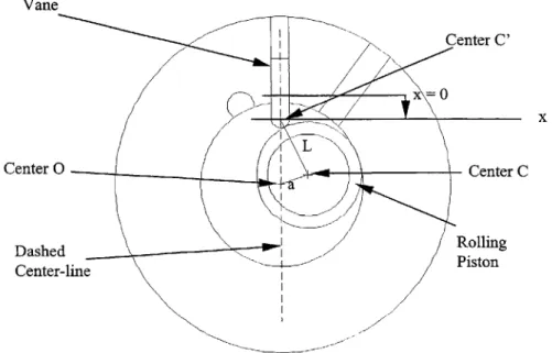
Figure 2.1 (Shows the slider-crank geometry of the rolling piston and the vane. Center C represents the center of the rolling piston, Center 0 represents the center of the crank

(25)

In Figure 2.1 it is easy to see that if the position of the vane as a function of time and crank angle 0 (see also Figure 2.2) can be found, then the position of the vane stem as a function of time and crank angle 0 is also known (they are equal). The parameters that are of concern are length a, length L, and o (angular speed of the shaft about Center 0). These parameters are listed below. They come from Carrier and apply to the model DB240 rotary compressor.

a = .199in (shaft eccentricity) L = .962in + .177in = 1.139in

(2.1) (2.2) Equation 2.2 represents the summation of the rolling piston outside radius and the vane tip radius respectively.

Rotational speed is 3600rpm = 60 rev/sec = 60 hertz, thus...

o = 2*(7)*f= 2*(3.14159)*60 = 377 rad/sec = angular velocity of crank shaft (2.3) f is the frequency and is equal to 60 rev/sec.

angle < angle 0 Center 0 x = 0 (Position of S C' at TDC) x Center C a

Figure 2.2 (Used for developing x(0) and x(t), where x is the distance from the position of C' at TDC to Center C' at time t)

(26)

a + L = x + L*(cos(4)) + a*(cos (0))

where x is the distance from the position of C' at TDC to Center C' at time t. It can also be seen that...

sin(#) = (a/L)*sin(0) (2.5)

From trigonometry...

cos2(#) + sin2

(#)

= 1 (2.6)

Now, by substituting Equation 2.5 into 2.6 and solving for cos(4) yields...

cos(#) = (1 - (a2/L2)*(sin2(0))1/2 (2.7)

Substituting Equation 2.7 into 2.4 and solving for x yields... x(6) = a + L - a*cos(0) -(L2

-a2 sin2()) 12 (2.8)

where x is the distance from the position of C' at TDC to Center C' at time t, 0 is the crank angle measured in radians, and a and L are the distance parameters described in Figures 2.1 and 2.2 which have values given in Equations 2.1 and 2.2 respectively.

In order to relate the crank angle (0) to the angular velocity (o) and time t, the following equation is used...

0 = o*t (2.9)

where t is the time measured in seconds.

Substituting Equation 2.9 into Equation 2.8 yields the following...

x(t) = a + L -a*cos(cot) -(L2 _-_a2 _sin2_(ot))112 _(2.10)

where x is the distance from the position of C' at TDC to Center C' at time t, o is the angular speed of the crank shaft which has a constant value given by Equation 2.3, a and L are the distance parameters described in Figures 2.1 and 2.2 which have values given in Equations 2.1 and 2.2 respectively, and t is the time in seconds.

It was decided that the latching of the vane stem will occur during approximately .020in of vane stem displacement from TDC. In order to set the parameters for the dynamic

analysis of the slider, the time period in which the vane stem is in the x = .020in range needs to be calculated. Using Equation 2.8 and employing trial and error techniques it

(27)

was found that at 0 equal to .43 radians x(0) was equal to .021in. Thus, this value of 0 met the design criteria well. Now, using Equation 2.11 below, the total time span for engaging the slider into the vane-stem latch can be calculated. Notice that the total time is multiplied by a factor of two to account for both the approach and departure of the

vane-stem from TDC.

t = (6/(o)*2 (2.11)

Where t is the time in seconds, 0 is the crank angle (.43 radians for the latching case), and to is the angular velocity of the crank shaft and is measured in radians/second (377rad/s, a constant value). Substituting these values into Equation 2.11 yields the following result...

t = .00228 seconds (2.12)

(28)

2.3 _{MOTION AND DYNAMIC ANALYSIS OF THE SLIDER PART 1}

Since the time required for engagement of the slider into the latch has been calculated (Section 2.2), a detailed dynamic and motion analysis of the slider is needed. This section will present the methods for solving the parameters that govern the dynamic analysis of engaging the slider into the latch. The maximum velocity of the slider will also be calculated for the purpose of friction analysis in Section 2.5. This section will conclude with a description of the necessary spring force specifications that are required to engage the slider. The following design criteria will be useful.

m = .0001657 (lb*s2_)/ft

= .00001381 (lb*s2)/in _(2.13)

dT = xl - x2=.070in (2.14)

t = .00228 seconds _(2.15)

Where m is the design mass of the slider, dT is the total travel needed for the slider to engage the latch, x1 represents the maximum coil spring compression displacement away from the relaxed position, x2 represents the minimum coil spring compression

displacement away from the relaxed position, and t is the time period in which the slider must engage the latch (Note that Equation 2.15 is equal to Equation 2.12).

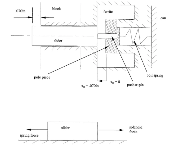
Figure 2.3, below, shows a general schematic that includes the main parameters that govern the slider motion. Note that this is not a detailed drawing of the

slider/spring/pusher-pin/pole piece system. However it will do fine for the purpose of obtaining the appropriate modeling equations.

(29)

.070in can coil spring Xss= .070in pusher-pin slider spring force solenoid force

Figure 2.3 (The top view shows the basic geometry for the modeling of the slider dynamics. Note the positive direction of displacement is away from the pole piece. x_ is

measured from the edge of the pole piece closest to the slider to the nearest edge of the slider. The bottom view shows a free body diagram of the slider when the solenoid force

(30)

can

coil spring pusher-pin

x, = 0

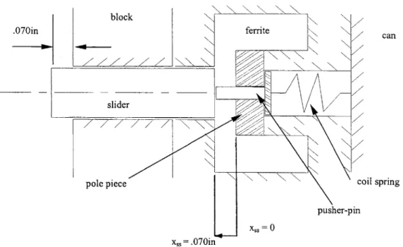
Figure 2.4 (This shows the slider in the fully disengaged position and up against the pole piece. xS is equal to zero in this schematic. Note that the spring is at maximum

(31)

can

pole piece N coil spring

pusher-pin

x,,=.070in

Figure 2.5 (This shows the slider in the fully engaged or latched position. The spring is now at minimum compression. Note the slider total travel dimension (x,, is equal to .070

inches here). The sign convention stays the same as in Figures 2.3 and 2.4.)

Thus, by looking at Figures 2.3, 2.4, and 2.5, _{the slider motion can be described as}

follows; the slider starts at a displacement value of x,, = Oin (fully disengaged) and travels a distance of .070in to end at a displacement values of x,,= .070in (fully engaged).

The first step in the analysis is to calculate the necessary engaging spring force. To do this the value of the spring constant, k, will be solved for. This will allow for the

specification of the linear force range that is needed to accelerate the slider into the latch within the time period specified by Equation 2.15. When the slider is having the spring force applied to it to engage the latch the solenoid force is zero (no voltage). At this point the spring is then free to push the slider in the positive xs direction (see Figure 2.4) away from the pole piece and into the latch. It is important to understand that the initial slider position is in contact with the pole piece. To set up the equation for the engaging analysis, Figure 2.6, below, will be used.

(32)

can Coill sp g slider pole piece pusher-pin _x_p= 0 XSP _xsp _.375in slider spring force

Figure 2.6 (The top view shows the slider/spring interface. Note the positive x,, direction is reversed from Figure 2.3 and applies to Equations 2.16 through 2.28 only. The bottom

view shows the free body diagram of the slider.)

Note that in Figure 2.6 the positive x, direction is reversed from that of Figure 2.3. This is done just for the modeling of the engaging of the slider. It applies to Equations 2.16 through 2.28 only. Once the appropriate spring force is obtained, it will be combined with the solenoid force and will have the sign convention shown in Figure 2.3.

Now, by applying Newton's law of motion to the slider spring combination...

mK S, + kq,= 0 _(2.16)

where m is the mass of the slider in (lb*s2_)/ft,

R S, is the acceleration of the slider in ft/s2,

k is the spring constant in lb/ft, and x, is the displacement of the slider away from the equilibrium position in ft. The general real solution of Equation 2.16 is...

x,,(t) = Acos[(k/m) 2_{(t)] + Bsin[(k/m)/} 2_(t)]

(33)

where x,,(t) is the displacement of the slider from the equilibrium position as a function of time, k is the spring constant in lb/ft, m is the mass of the slider in (lb*s2_)/ft,_{t is the}

time in seconds, and A and B are arbitrary constants that must be solved for by applying boundary conditions. Now in order to solve Equation 2.17 for k, the following boundary conditions must be applied.

Intial Boundary Conditions: m= .0001657 (lb*s2_)/ft

= .00001381 (lb*s2)/in (2.18)

t = 0 (2.19)

x1 = .0208ft = .250in (2.20)

dx,,/dt = 0 ft/s (2.21)

By substituting these values into Equation 2.17 the arbitrary constants A and B can be solved for.

A = .0208ft = .250in (2.22)

B=0 (2.23)

The initial boundary conditions apply to the slider with the spring under maximum compression (in the direction of positive xS, in Figure 2.6). Note that the assumed value of x1 (Equation 2.20) was chosen in an effort to obtain a practical value of k, the spring constant, that is feasible based on the design and geometry constraints of the spring. Once k is calculated, the maximum compression force, the minimum compression force and the linear range of force needed to accelerate the mass will be known.

The final boundary conditions are listed below.

t = .00228 seconds (2.24)

x2 =.015ft =.180in (2.25)

These final boundary conditions represent the time required to engage the slider into the latch (note that Equation 2.24 = Equation 2.15 = Equation 2.12) and also specify the total slider travel length (.070in = xl -x2).

By substituting Equations 2.22, 2.23, 2.24, and 2.25 into Equation 2.17, k can be solved

for.

(34)

Now, in order to calculate the maximum velocity of the slider the equation of velocity as a function of time needs to be calculated. Taking the derivative of Equation 2.17 results in...

dx,,/dt = A*[(k/m)11 2 _{(-sin(t*(k/m)"}2_{)] + B*[(k/m)1'}2 _{cos(t*(k/m)l'}2_)] _(2.27)

where dx,,/dt is the velocity of the slider in ft/s, A and B are the arbitrary constants given in Equations 2.22 and 2.23 respectively, m is the mass of the slider in (lb*s2_{)/ft, k is the}

spring constant given in Equation 2.26 in lb/ft, and t is the time in seconds. The

maximum velocity of the slider will occur just before the slider becomes latched (at t =

.00228s). Substituting Equations 2.18, 2.22, 2.23, 2.24, and 2.26 into Equation 2.27 yields the following result.

u = - 4.443 ft/s = - 58.6 in/s (2.28)

Equation 2.28 represents the maximum velocity obtained by the slider. Note that the negative sign is correct according to the sign convention given in Figure 2.6. These values will be positive when used later in accordance with the sign convention described in Figure 2.3.

By multiplying Equation 2.26 by Equations 2.20 and 2.25 the linear force range can be obtained.

S1 = .393 lb (2.29)

S2 = .283 lb (2.30)

SI represents the force the spring must apply under maximum compression (slider fully disengaged and against the pole piece). S2 represents the force the spring must apply once the slider is completely engaged or latched. The spring forcing function is linear with respect to displacement and has a slope defined by Equation 2.26. Both of these force values are positive with respect to the x,, direction given in Figure 2.3.

(35)

2.4 MOTION AND DYNAMIC ANALYSIS OF THE SLIDER PART 2

This section concludes the motion and dynamic analysis of the slider by combining the spring force and the solenoid force for the disengaging of the slider. This section is split into two parts. The first part covers the first solenoid design which included a permanent magnet. The majority of the analytical work was done on this design. The second part covers the new and existing solenoid design which does not include a permanent magnet. The objective of this section is to calculate the necessary solenoid force needed to

completely disengage the slider from the latch in the time period given by Equation 2.12. This section will conclude with a detailed description of the force values calculated for the first solenoid design and an operating description of the second solenoid design. It is important to note that all references to "positive force" and "negative force" in this

section will be according to the sign convention shown in Figure 2.3 in Section 2.3. SOLENOID DESIGN 1: USING A PERMANENT MAGNET

In order to calculate the necessary energized magnet force needed to disengage (or unlatch) the slider, the relationship between the permanent magnet force and the spring force must be fully understood. Table 2.2, below, lists experimentally obtained force values acting on the slider from the permanent magnet. It also lists the spring force values calculated in Section 2.3 as well as the permanent magnet force values multiplied by a constant (2.25). These 2.25x values will be used as a first order analysis for modeling the extraction of the slider with an energized magnet. The basis for multiplying the

permanent magnet force values by a constant came from the advice of Dr. Steve Umans. Having had previous experience with solenoids, he figured that the true energized magnet would reflect similar force versus displacement data as the non-energized permanent magnet but at just a higher magnitude. The actual value of 2.25 was chosen simply because it is physically possible to energize the permanent magnet to 2.25 times the values shown in the second column of Table 2.2. Also it serves as a good starting point for the iteration process because it "looks" like it may work. The values in Table 2.2 are used in Figures 2.8 and 2.9. Listed in Table 2.1 are some of the specifications for

Solenoid Design 1.

Table 2.1 (Specifications of Solenoid Design 1)

Resistance Value (ohms) 6.5

Type of Winding Single wound

Operating Voltage 35+

Type of Wire Number 28 (insulated)

(36)

Table 2.2 (Experimentally Obtained Force vs Displacement Values For Solenoid Design 1)

Displacement x, (in) Permanent Magnet Spring Force From 2.25x Permanent (x, is measured from Force (ib) Section 2.2 (ib) Magnet Force

the edge of the perm. (lb)

magnet to the edge of the slider) 0 1.53 3.4425 .028 1.055 2.374 .04 .393 .053 .697 1.568 .07 .548 1.233 .085 .359 .8078 .106 .307 .6908 .11 .283 .124 .216 .486

(37)

.070in

can

magnet force

Figure 2.7 (This design is used in Solenoid Design 1 Notice that for this analysis x is measured from the edge of the permanent magnet to the edge of the slider. This schematic

(38)

Frcevs spamenIRt 1.8 1.6 1.4 1.2 1 + Sprng Fance (1b) Frm Mg Farce(b) 0

2 0.8 Ry. (Ferm rvWg. Facoe(b))F

U. - Liera (Spring Fare (1b))

0.6

0.4 02

0

0 0C2 04 0.06 0OB Q.1 12 (.14

Sicdr Dlsplaemrt (in)=

Xs

Figure 2.8 (This shows the linear force curve of the spring and the experimentally obtained data points which correspond to the permanent magnet force on the slider.)

For this disengaging analysis, x, is the distance measured between the edge of the permanent magnet and the edge of the slider with the positive direction indicated in Figure 2.7. Thus, by looking at Figure 2.7, it can be concluded that the slider is fully disengaged (unlatched) at a displacement value of x, equal to .040in (since the spacer is .040in thick). Note that in this first design the pole piece shown in Figure 2.3 was replaced with a non-magnetic spacer that was .040in thick. Also, in place of the pusher-pin, there was a permanent magnet that was in contact with the spacer. See Figure 2.7 above.

So in Figure 2.8 the slider starts at a displacement value of x, = .040in and travels a distance of .070in to end at a displacement value of x, = .11 in (the slider is in the fully latched position here). Notice that the permanent magnet force is higher than the spring force at a displacement value of .040in. This is to allow the permanent magnet force to hold the slider in the unlatched position until the permanent magnet field is killed by application of current to the coil in the demagnetizing direction. When the permanent magnet field is killed the permanent magnet force values in Figure 2.8 go to zero. This allows the spring to engage the slider in the latch as described in Section 2.3. Once the

(39)

slider has become latched the permanent magnet field is restored. Notice, at this latched position, that the spring force is greater than the permanent magnet force keeping a net positive force on the slider. This ensures that the slider will not come unlatched.

In order to disengage the slider from the latched position, the magnet force must become greater than the spring force. In fact, the magnet force must be large enough to ensure that the slider becomes fully disengaged in a time period of .00228 seconds (Equation 2.12).

Foice vs Uspacment Inducing 2.25x Pen Mg. Aid Spring

= 70.839x3 + 147.258x2 -43.0515x + 3.447 3.5 3 B" 2.5 + Seies1 s Series2 e2 -Unear (Series1) oL 1.5 -1.5 -Fy. (Seies2) 1 0.5 0 0 0.02 0.04 0.06 0.08 0.1 0.12 0.14

Figure 2.9 (This shows the linear force curve of the spring and a possible energized magnet curve (2.25x ) that was fit using a third order polynomial.)

In Figure 2.9 the energized magnet force versus displacement data has been plot and has been curve fit using a third order polynomial. This energized magnet force versus displacement plot represents magnet force values of 2.25 times those given in Figure 2.8 above. This method of simply multiplying the experimentally obtained permanent magnet force values by a constant is done as a simple approximation. Dr. Steve Umans did a Finite Element Analysis (FEA) of this first design and that is covered later. The linear spring force versus displacement has also been plot. The first equation is...

FE = 70.839x 3_{+ 147.258x}2 _-_43.0515x,₊_3.447 _(2.31)

(40)

where FE is the energized magnet force (1b) and x, is the displacement away from the permanent magnet (in) according to the sign convention given in Figure 2.7.

The linear equation governing the spring force as a function of displacement is also given below...

S3 = -1.5714x, + .4559 (2.32)

where S3 represents the spring force (lb) and x, is the displacement away from the permanent magnet (in). Equation 2.32 comes from the values calculated in Section 2.3 and listed under Equations 2.26, 2.29, and 2.30.

In order to model the dynamics of the slider being disengaged Figure 2.7 will be referred to. Applying Newton's law of motion to the slider, the spring force, and the energized magnet force yields the following equation...

mi S3 + FE =0 (2.33)

where m is the mass of the slider (lb*s2_{/ft) whose value is given in Equation 2.13, R, is}

the acceleration of the slider (second derivative of displacement with respect to time), S3 is the spring force function given in Equation 2.32 , and FE is the energized magnet force function given in Equation 2.31. Substituting the values in Equations 2.31 and 2.32 into Equation 2.33 yields the following.

mi, - ( -1.5714x, + .4559) + (70.839x, 3 + 147.258x,2 - 43.0515x, + 3.447)= 0 (2.34) Simplifying Equation 2.34 and reducing the order of the differential equation to a system of two first order equations results in the following...

mi + (70.839)x, 3 ₊_(147.258), 2

+ (-41.480)x, + 2.9911 = 0 (2.35) where m is the mass of the slider (lb*s2_/ft), _{is is the reduction term which is the first}

derivative of displacement with respect to time, and x is the displacement of the slider away from the magnet (in) according to the sign convention given in Figure 2.7. Even though the differential equation was simplified into the form shown in Equation 2.35 above, it represents a nonlinear system which proves highly nontrivial to solve by hand. Therefore, this equation was solved using a numerical solving technique in MATLAB. The MATLAB code is listed in the Appendix. In order to understand the variables a,, b,, c,, and d, in the MATLAB code the following equation form was adopted.

(41)

For the given FE, the constants as, b,, c,, and d, are listed below.

a, = 70.839 _(2.37)

b, = 147.258 (2.38)

c,= -41.480 (2.39)

d5= 2.9911 (2.40)

Solving the first order system of differential equations given in Equations 2.35 using MATLAB gives a net slider displacement of .080in in a time span of .0023 seconds. This clearly indicates that if the energized magnet extracting force can realistically reach the values demonstrated in Figure 2.9 then Solenoid Design 1 will work.

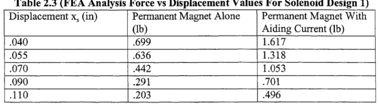
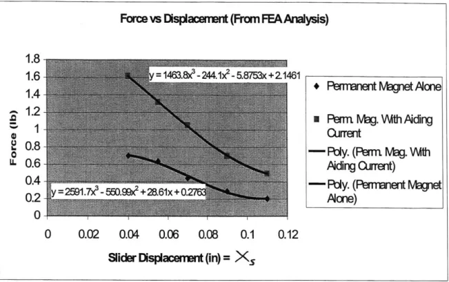
In an effort to obtain a more accurate model of the energized magnet extracting force Dr. Steve Umans did a FEA analysis on Solenoid Design 1. In order to reduce the number of iterations that would have to be run, he set the analysis to achieve a force of .4861b at a displacement of x, equal to .11 Oin. This parameter was chosen as a starting point by looking at the 2.25x permanent magnet force value at a displacement of x, equal to .124in (see Table 2.2). The results of Dr. Umans analysis are shown below in Table 2.3 and Figure 2.10.

Table 2.3 (FEA Analysis Force vs Displacement Values For Solenoid Design 1) Displacement x, (in) Permanent Magnet Alone Permanent Magnet With

(lb) Aiding Current (lb) .040 .699 1.617 .055 .636 1.318 .070 .442 1.053 .090 .291 .701 .110 .203 .496

(42)

Force vs Displacement (From FEAAnalysis)

1.8

1.6 =1463.8x- 244.1x2_{-5.8753x+2.1461}

1.4+ * Fmnnent Magnet Aone

1.4 n

~1.2

1 PernMag. Wth Aiding

*0.

02 0.8 _- Ry. (Perm Mag. _WtIh

LL 0.6 _{Aiding Current)}

0.4 -29.) Ri,6xO.Py. (Fwm~nent Magnet

0.2 Aone)

0

0 0.02 0.04 0.06 0.08 0.1 0.12 Slider Displacement (in) =

Xs

Figure 2.10 (This plot shows the Force vs Displacement values shown in Table 2.3 above. Displacement is equal to xhere also. These values represent the FEA analysis

on Solenoid Design 1)

The values in Figure 2.10 were also curve fit using a third order polynomial. Those equations are shown above in Figure 2.10. Using the same analysis technique on the FEA values as was demonstrated in Equations 2.31, 2.32, and 2.33 and using the same value

for S3 (the spring force does not change) results in the following equations...

FE = 1463.8x 3 - 244.1x2 - -5.875x, + 2.146 (2.41)

Where FE now represents the energized magnet force (lb) using FEA values and x, is the displacement of the slider away from the permanent magnet (in). Substituting the values in Equations 2.32 and 2.41 into Equation 2.33 results in the following equation...

mi, - (-1.5714x,+ .4559)+ (1463.8x3 -244.1x 2 _-_{5.875x, + 2.146)}

= 0 (2.42)

Simplifying Equation 2.42 and reducing the order of the differential equation to a system of two first order equations results in the following...

(43)

mi,+ (1463.8)xS3 ₊_(-244.1)x, 2

+ (-4.3039)x, + (1.6902) = 0

where m is the mass of the slider (lb*s2_{/ft) whose value is given in Equation 2.13, i, is} the acceleration of the slider (second derivative of displacement with respect to time), S3 is the spring force function given in Equation 2.32, 1, is the reduction term which is the first derivative of displacement with respect to time, x, is the displacement of the slider away from the permanent magnet (in) according to the sign convention given in Figure 2.7, and FE is the energized magnet force function given in Equation 2.41.

By using the format shown in Equation 2.36 the new values for a,, b,, c,, and d, can be found.

as= 1463.8 (2.44)

b= -244.1 (2.45)

c, =-4.3039 (2.46)

d= 1.6902 (2.47)

Using these new FEA based values to solve the differential equation given in Equation 2.43 gives a net slider displacement of .0515in in a time period of .0023 seconds. Once again MATLAB was used to solve Equation 2.43. This new displacement result is lower than the required .070in of slider travel needed in .0023 seconds. This indicates that the slider will not come unlatched during one revolution of the rolling piston.

At this point it was decided the best thing to do was to go ahead and put the latch

mechanism together and test it with Solenoid Design 1. As is discussed in Chapter 4, the results of Solenoid Design 1 proved unsatisfactory. The above FEA analysis, with its predicted unsatisfactory result, would prove to be the case in real world testing. Other problems were also discovered relating to the permanent magnet and the high operating temperatures of the compressor.

(44)

SOLENOID DESIGN 2: NO PERMANENT MAGNET AND DOUBLE WOUND COIL

Table 2.4 (Specifications of Solenoid Design 2)

Resistance Value (ohms) 1.8

Type of Winding Double wound

Operating Voltage (V) 25

Type of Wire Number 28 (insulated)

Permanent Magnet No

Due to the inability of Solenoid Design 1 to properly extract the slider in .0023 seconds and also due to other problems, it was decided to adopt a different solenoid design. With the aid of Professor Wilson and Dave Otten, it was experimentally determined that

Solenoid Design 1 was not producing enough extracting force. In order to obtain more extracting force a new, double wound solenoid design was adopted. By double winding the coil the basic wire cross section was doubled and the length of wire that could be wound in the given volume of the coil was cut in half. This lowered the total resistance of the coil by approximately 70% (see Tables 2.1 and 2.4). By applying the same voltage to Solenoid Design 2 as was applied to Solenoid Design 1 the current used by Solenoid Design 2 was now larger in magnitude (Since Voltage = Current * Resistance). This allows Solenoid Design 2 to produce more unlatching force on the slider with the same magnitude of applied voltage to the solenoid coil.

Due to the time constraint that the project was under, no official analysis was done on Solenoid Design 2 to determine the extracting force acting on the slider as a function of displacement. Instead, the solenoid was simply built according to the specifications given in Table 2.4 and experimentally tested in the latching mechanism. As is discussed in Chapter 4, this design also proved somewhat unsatisfactory. It appeared that the solenoid was unable to extract the slider within one stroke of the compressor. Dr. Umans simply doubled the time (from .020 seconds to .040 seconds) that the unlatch voltage signal is applied to the solenoid. This adjustment appears to have worked and the solenoid is now able to unlatch the slider consistently.

(45)

2.5 ANALYSIS OF FRICTION ON THE OPERATION OF THE

SLIDER

The objective of this section is to calculate the maximum resistive force acting on the slider as it is in motion to engage the latch. The slider and the entire latch mechanism operate in an oil and refrigerant 22 saturated environment. Thus the important parameter is to calculate the sliding resistance due to the presence of an oil film surrounding the slider.

Of use will be the following parameters...

b = .003in = .00025ft (2.48)

u = 4.883 ft/s = 58.6 in/s (2.49)

where b is the clearance distance between one side of the slider and the slot in which it travels and u is the maximum velocity of the slider (from Equation 2.28).

It can be seen from Figure 2.11 that the part of the slider that will have a resistive force applied to it is the rectangular part with dimensions .240in X .1 00in X .400 in (.240in into the page and .1 00in thick). This rectangular part is the part that guides the slider during latching and unlatching. It is also the load bearing part during the time in which the slider is latched. Figure 2.11, below, shows a simple front view of the slider and the slot it travels in and labels the part that has the resistive force applied to it.

(46)

block / 7 _/ / _/ 77 -7 7 7/ .330in 0 .070in slider .264in

applied here slot for slider to travel in

Figure 2.11 (This shows a simplified front view of the slider and the slot in which it travels. The top view shows the unlatched position while the bottom view shows the

latched position. The rectangular part has dimensions .400in X .1 00in X .240in.)

Notice that the slot that the slider travels in is only .330in in length however. This reduces the net surface contact area for sliding resistance to...

Asur = [(.330in)*(.240in)*2] + [(.330in)*(.l00in)*2] =

2244in2 ₌_.00156ft2

(2.50) where A,,, is the total surface area affected by sliding resistance.

Figure 2.12, below, shows a viscous fluid trapped between two plates. The top plate has a force applied to it and is traveling with a constant velocity while the lower plate is fixed. This figure will be used to set up the governing equations needed to calculate the net resistive force on the slider.

(47)

Upe Pltz u a Viscous Fluid Velocity Profile dP/dg = 0 g Fixed Plate _I

Figure 2.12 (This shows a viscous fluid between two parrallel plates. The top plate has a force F applied to it and it has a constant velocity u. The bottom plate is fixed. Note the

sign convention)

In Figure 2.12, above, it is assumed that there is no pressure gradient in the g direction. In other words dP/dg = 0. The resisting force on the upper plate can written as...

F = t*Am (2.51)

where F is the resisting force on the upper plate, - is the shearing stress of the fluid, and Am1 is the surface area of the upper plate or slider. The shearing stress is defined by...

t = p*(du/dh) (2.52)

where pL is the viscosity of the fluid and du/dh is the velocity gradient of the fluid between the two plates. The variable du/dh can be defined as follows...

du/dh = u/b (2.53)

where u is the velocity of the top plate (or maximum velocity of the slider) and b is the distance between the two plates. For the case of the slider, the velocity gradient between the two plates will be considered linear. The value of the viscosity of the oil/refrigerant 22 mixture came from a Daniel plot of Zerol 300/R22 at a pressure of 170psia and a temperature of 90 degrees F, and is given below in Equation 2.54. This temperature and pressure represents a good average operating condition for the vane-latching mechanism.

p = 1.0737 x 10~ (lb*s)/ft2 _(2.54) F b h

L

Upper Plate u

(48)

Now that the viscosity of the oil/refrigerant 22 mixture has been found, the velocity gradient between the upper and lower plate can be found. Substituting Equations 2.48 and 2.49 into 2.53 results in

du/dh = _{[4.883 ft/s]/.00025ft}₌_{19532.0 1/s} _(2.55)

where du/dh represents the velocity gradient of the oil/refrigerant 22 fluid between the surface of the slider and the slot in which it travels. Note that the velocity value of 4.883 ft/s in Equation 2.55 represents the maximum velocity of the slider found in Section 2.3. Now, substituting Equation 2.54 and Equation 2.55 into Equation 2.52 results in the

following... -r= .2097 lb/ft2

(2.56) where c represents the shearing stress of the oil/refrigerant 22 fluid at the interface of the slider. One final substitution of Equation 2.56 and Equation 2.50 into Equation 2.51 results in the final result...

F = (.2097 lb/ft2_)*(.00156ft2

) = .000327 lb (2.57)

where F represents the maximum resistive force acting on the slider as it is in motion to engage the latch. In relation to the spring and magnet forces needed to engage and disengage the slider, this force is small enough to be considered negligible.